A directed walk in probability space that locates mean field solutions to spin models
Abstract
Despite their formal simplicity, most lattice spin models cannot be easily solved, even under the simplifying assumptions of mean field theory. In this manuscript, we present a method for generating mean field solutions to classical continuous spins. We focus our attention on systems with non-local interactions and non-periodic boundaries, which require careful handling with existing approaches, such as Monte Carlo sampling. Our approach utilizes functional optimization to derive a closed-form optimality condition and arrive at self-consistent mean field equations. We show that this approach significantly outperforms conventional Monte Carlo sampling in convergence speed and accuracy. To convey the general concept behind the approach, we first demonstrate its application to a simple system - a finite one-dimensional dipolar chain in an external electric field. We then describe how the approach naturally extends to more complicated spin systems and to continuum field theories. Furthermore, we numerically illustrate the efficacy of our approach by highlighting its utility on nonperiodic spin models of various dimensionality.
I Introduction
Classical spin models constitute a ubiquitous tool in physical sciences due to their abilities to describe the features and phase behaviors of a wide variety of different physical systems. Many properties of these systems can be efficiently understood by applying the mean field (MF) approximation, where each spin is assumed to interact with a static environment determined self-consistently to represent the average. In isotropic systems, such as the periodically replicated Ising model, all spins are statistically identical. The mean field solution can therefore be captured within a single self-consistent equation. By contrast, anisotropic systems, such as those containing an interface, give rise to a more complicated multidimensional array of equations. When formal solutions to these equations are inaccessible, for example by their transcendental nature, they can be evaluated algorithmically with adaptive sampling schemes. Even in the mean field case, however, typical sampling schemes involve a stochastic walk of some sort in the system configuration space, which becomes prone to frustration as the system size and heterogeneity increases.
In this manuscript, we eliminate such frustration by establishing, instead, a deterministic walk in the space of configurational probabilities. As we demonstrate, this approach converges rapidly and can be designed to target the correct mean field solution. Our approach utilizes the joint framework of directional statistics and variational optimization. The underlying information-theoretic perspective paves a contextualized and accelerated way to study the properties of a wider class of spin models encountered in statistical mechanics, theoretical neurobiology, and artificial intelligence.
Spin systems are capable of modelling specific functionalities and revealing fundamental insights for diverse phenomena that occur in condensed phase systems. Jasnow and Wortis 1968; Fröhlich and Lieb 2004; Evans et al. 2014; Budkov et al. 2020 For instance, a monolayer rotor model provides a mechanistic explanation of magnetization reversal observed in magnetic materials Hinzke and Nowak 1998; Hinzke and Nowak 2000, while water diffusion and proton conduction in nanopores can be described by a discrete charge model on a segmented lattice Dellago et al. 2003; Köfinger et al. 2008; Köfinger et al. 2009. In practice, it is nearly impossible to solve a designated spin model exactly, except in a handful of pedagogical cases Chandler and Wu 1987; Baxter 1982 where the system equilibrium weight can be decomposed into computable subsystem weights according to a simple spin connection topology. When such a decomposition is unavailable, an approximate decomposition can be accomplished via mean field theory, which serves as a zeroth order approximation to the exact theory.
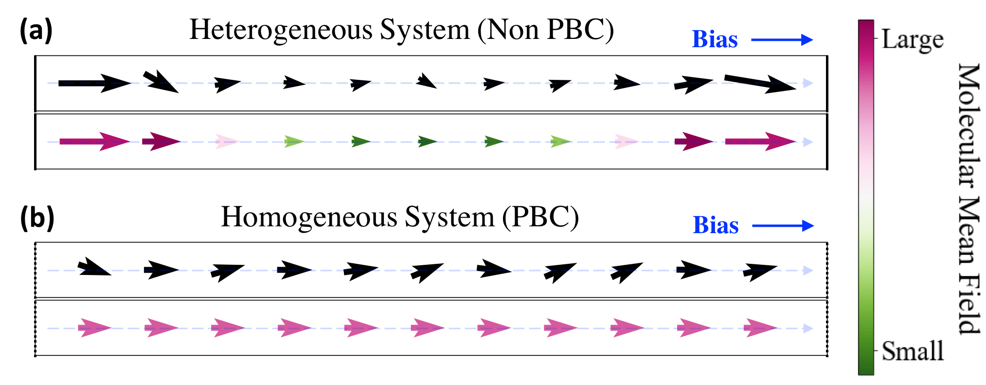
Notably, the complexity of a given spin model is set by the length scale of spin-spin interactions. When the interactions remain highly local, as in the standard nearest-neighbor Ising model, the majority of spins in the system can be treated as statistically independent. The resulting anisotropic mean field equations are hence weakly coupled. For long-range interactions, such as those occurring between the charged species, the growing cross-dependence of these coupled equations poses a challenge for obtaining exact solutions, even with statistical correlations removed by the mean field assumptions. Figure 1 highlights this additional complexity from anisotropy and long-range interactions: the former gives rise to a unique mean field equation for each lattice site and the latter makes the spin topology computationally irreducible. In principle, one may overcome the associated challenge by employing stochastic sampling methods that bias towards the thermodynamically relevant system configurations. Unfortunately, such methods can fail to converge, especially in cases where the number of metastable basins in the energy landscape proliferates. Kirkpatrick et al. 1983; Neal 1996
In this manuscript we focus our attention on the mean field analysis of finite heterogeneous spin systems. In particular, we utilize the well-known Gibbs-Bogoliubov-Feynman variational inequality Chandler and Wu 1987; Falk 1970; Callen 1985 and reframe the mean field approximation as a constrained optimization on the free energy functional of configurational probabilities. We reexpress the infinite-dimensional optimization as an equivalent finite-dimensional optimization over a compact set in the Euclidean space that contains the mean spin characters. The latter problem can be easily solved recursively. We show that this procedure leads to a class of self-consistent mean field equations that are otherwise difficult to derive analytically, and we prove that the iterative procedure is guaranteed to converge.
Our approach invokes the concept of Markov random fields, also known as factor graphs. Kindermann et al. 1980 This generalized variant of lattice model prescribes adjacency relations between a cloud of random variables, as edges between nodes of a graph, based on their conditional dependence. Modeling physical spin systems using graphical networks is practically advantageous due to the factorizability native to the accessible system degrees of freedom. That is, the joint distribution of a cluster of variables (e.g., spin configurations) can be factorized as a product over elemental weighting functions (e.g., potential energy surface), each of which involves relatively few variables. Recent progress has been made on the theoretical and practical aspects of Ising model as factor graph through the variational perspectives. Dembo and Montanari 2010; Jain et al. 2018; Koehler 2019 Here we demonstrate the ubiquity of fast convergence associated with the mean field iterative approach. For illustrative purposes, we examine a trivial representative model composed of a finite chain of freely rotating dipoles. Even this simple model yields a multimodal energy landscape that can frustrate standard methodologies. Despite the simplicity of this illustrative model, we note that the same analysis can be applied to a wider range of more complex spin models, as we discuss later in our manuscript.
The manuscript is organized as follows. In Section II, we introduce the one-dimensional dipolar lattice as a minimal model with a smooth and continuous multimodal energy landscape. Section III briefly reviews the mean field formalism in the information-theoretic context. In Section IV, we simply state, without proofs, the form and applicability of our mean field iterator. Section V entails a derivation of the iterator for solving the dipolar model and presents approximation theorems for which relevant model parameters control the iteration convergence. We then address spin models with more general state spaces and interactions in Section VI, and expand the analogies to include continuum field theories. In Section VII, we numerically justify the efficiency and stability of the method outlined in Sections V and VI by examining the mean field convergence for various systems, ranging from the one-dimensional dipolar chain to the three-dimensional Heisenberg slab.
II Model Description
II.1 Restriction on model space
We first point out that the concept presented within the work is not model specific, i.e., we will be able to systematically generate directed walks in the space of configurational probabilities for general classical spin models, provided that there is a symmetry associated with each spin degree of freedom. In some cases, we may exploit this symmetry even when the model Hamiltonian contains an external field contribution that enthalpically breaks the symmetry.
For concreteness, we first discuss how the approach applies to a simple finite dipolar chain.
II.2 Illustrative model: finite dipolar chain
Let us consider a reference system of interacting dipoles on a finite one-dimensional regular lattice, , which we assume to extend in the -Cartesian direction. Each dipole has a fixed magnitude, , and can rotate freely within a two-dimensional plane as sketched in Fig. 1. Under the point-dipole approximation, the interaction between dipoles and is,
| (1) |
where denotes the orientation of dipole , indicates the unit vector separating dipoles and , and is the separation distance. The indices specify position along the lattice so that for lattice constant of . The system Hamiltonian is,
| (2) |
where specifies the angular configuration of dipoles and the second term describes the influence of external electric field, .
With fixed temperature, lattice size, and number of dipoles, the canonical partition function is given by,
| (3) |
where the integral spans all possible dipole configurations and is the Boltzmann constant times temperature. This relationship defines a free energy , yet the equilibrium measure is computationally intractable for all but the smallest system sizes due to the high-dimensional integral . Such intractability can be typically circumvented by either biased subsampling or the application of mean-field theory (MFT).
Biased subsampling takes advantage of the fact that in many cases is dominated by a small subset of low energy configurations. Sampling these configurations, e.g., via Monte Carlo algorithms, typically enables asymptotic convergence of equilibrium properties, despite that these techniques are prone to frustration in systems with nonconvex free energy landscape. Application of MFT, on the other hand, reduces computation by creating a model system with dramatically simplified configuration probabilities and a corresponding free energy that can be variationally related to that of the target system, i.e., . A major advantage of MFT is that the model system is often solvable through numerical or analytical methods.
III Mean Field Formalism
In MFT, the fluctuating environment is modeled by a static mean field. Because the neglected fluctuations are entropically favorable, the free energy of the mean field system represents a loose upper bound on that of the interacting system. The trade-off in accuracy is that MFT significantly reduces the complexity and system size scaling associated with the computation of system properties.
For the lattice dipole system, the mean field free energy can be expressed parametrically as,
| (4) |
where the vectors and contain the mean orientations, , and polarizations, . In Eq. 4, the enthalpic term, , is simply the average system energy. The entropic term, is a sum of single dipole entropies (reflecting the lack of dipole correlations),
| (5) |
where labels the entropy of dipole dictated by an angular distribution . The distribution in Eq. 5 denotes the unique maximum entropy distribution commensurate with the mean , derived as the extremal of the action,
| (6) |
where the Lagrange multipliers enforce the normalization and the first moment constraint. Specifically, the maximizing , also known as a von Mises distribution, takes the form,
| (7) |
where gives the angular mean as expected for consistency, sets the angular fluctuation under an averaged field for which is a differentiable function satisfying the Riccati equation with initial condition , and in the normalizing constant denotes the zeroth order modified Bessel function of the first kind. The behavior of the function is shown in Fig. 2.

IV Main Result and Applicability
In essence, the mean field approximation limits the space of possible angular distributions to those satisfying Eq. 7 (discussed further in Appendix A). This limitation significantly reduces the search space for the optimization of in Eq. 4. However, even in this reduced search space, may exhibit metastable minima that prevent typical optimization routines, such as gradient updates, from reaching the global minimum. Our goal here is to outline a robust procedure that, when properly initialized, will reliably converge to the optimum under the mean field approximation. We formulate the procedure in terms of a mean field iterator, , which generates directed walks in the MF state space, i.e.,
| (8) |
where the index labels the iteration step. In our case, we consider such that on all lattice sites, such as would result from a voltage drop across the lattice driven by a pair of electrochemical reservoirs. This assumption will be kept implicit throughout the remaining sections.
Here, we provide a summary of our approach. Relevant key ideas are presented by order in the next sections, while technical details are described in their entirety within the Appendix. Under our assumptions, the explicit form of the iterator, , in Eq. 8 is given by,
| (9) |
which guides directed walks in MF state space. For the dipolar model, is the function appearing within Eq. 7 and illustrated in Fig. 2, whereas
| (10) |
represents the strength of molecular mean field experienced by dipole . We will show that the mean fields all point in the direction and depend only on the -components of the dipole averages. The iterator follows from minimization of the free energy and is constructed step by step in Secs. V.1-V.2, while its convergence is established in Sec. V.3.
The results for dipolar chain extend to other classes of spin models for which spin-spin interaction orients favorably along direction of the imposed external field (ferromagnetic models with consistent external field are thus canonical examples), as is elaborated in Sec. VI.1. Our lattice description then motivates a discussion on the continuum fields in Sec. VI.2.
V Iterator and Its Convergence
V.1 Global optimizer
Certain symmetries that are inherent to dipolar (spin-spin) interactions result in a significant reduction of the search space in the optimization of . Our construction of the MF iterator, , exploits these symmetries, which are formalized as the lemma below.

Lemma 1.1. A global maximizer of
| (11) |
satisfies for all .
Sketch of proof. Here we convey the central idea of the proof. An elaborated proof can be found in Appendix B.
We first recognize the invariance of the entropies under the partial reflections,
| (12) |
which can be realized through circular shift of the angular distributions and diagrammatically understood in Fig. 3(a). For a mean configuration , we consider such reflections on all sites and denote the partially reflected mean configuration by .

The operation leads to an energy reduction since it induces favorable dipolar couplings and encourages dipole alignment with the external field as depicted in Fig. 3(b). In Fig. 4, we show the reduction by plotting the full range of coupling values for two dipoles (Fig. 4) and the change in coupling from single dipole reflection (Fig. 4). Therefore, and .
In fact, the global maximum is attained only when the mean dipoles align with the external field.
Corollary 1.2. for all .
V.2 Mean field iterator
The MF iterator is a state-space operator that generates discrete flow towards the optima of . We use results in the previous section to derive its form. Although the parametrized distributions and free energy function are most naturally expressed in the polar coordinate, it is advantageous to consider a Cartesian frame where one of the axes points in the external field direction . With this coordinate change,
| (14) |
the projections can be isolated and treated separately. Now taking for the MF optimization in Eq. 4, we arrive at an array of self-consistent equations that manifest the first-order condition ,
| (15) |
where the matrix encodes the dipolar coupling,
| (16) |
with denoting the Kronecker delta, accounts for the local external fields, and gives the single dipole entropies,
| (17) |
with nondimensional polarity characterizing the angular dispersion. Let be the paired coordinates in shorthand so Eq. 15 can be arranged as a matrix equation,
| (18) |
where the matrix composed of blocks,
| (19) |
accommodates the collective anisotropic interaction in the dipolar chain, contains the augmented external fields, and
| (20) |
designates the entropic forces.
Eq. 18 defines the state-space property of the MF solution, , and can be utilized to ensure that is a fixed point of . Ideally, one would convert Eq. 18 into the form and analyze the associated fixed-point iteration. However, due to the noninvertibility of the partitioned matrix and entropy gradient , instead, we refer to Corollary 1.2 in Sec.V.1 and consider the dimensionally reduced through a projection of Eq. 15 onto the “important" subspace ,
| (21) |
where the molecular field acting on dipole can be explicitly defined through Eq. 21 after we project out half of the equations satisfied vacuously, i.e., . Hence we obtain our expression of the MF iterator,
| (22) |
where since . We then define in a component-wise manner. Clearly the properties of depend on the dipolar model parameters , and again we assume throughout the rest of the work. For practicality, we proceed to establish theoretical bounds on the convergence of by resorting to the approximation theorems below.
V.3 Convergence theorems
Our first theorem states that the iteration generated by converges uniformly under strong external field, regardless of the initial condition.
Theorem 2.1. There is an external field such that if entry-wise, the MF iterator,
| (23) |
with any initial estimate will converge linearly to the MF solution as the unique fixed point. That is,
| (24) |
where
| (25) |
gives the vector -norm for integer , denotes the repeated application of , and is a -dependent bound controlling how rapidly Eq. 23 converges towards the MF solution, up to a constant set by the initial condition as written on the RHS of Eq. 24. decreases with , reaching zero as , and is sensitive to dipolar model parameters. When and , a possible choice is .

Sketch of proof. When is sufficiently large, we expect due to dielectric saturation. We prove the theorem by showing that is contractive, namely any pair of states gets mapped closer to each other under so eventually as illustrated in Fig. 5. The update in this regime is monotonic as improves after each additional iteration (See Appendix B).
Now we examine the convergence when the external field is weak and does not exhibit any scaling with the system size. In particular, we follow Koehler’s approach Koehler 2019 by exploiting curvature of the MF free energy surface and deliberately picking out a subdomain of initial estimates. The following lemma counts the number of fixed points in the MF state space, which helps eliminate ambiguity when we specify suitable initial estimates in our next theorem.
Lemma 2.2. yields either zero or one fixed point in the interior of its domain.
Sketch of proof. Suppose that we find two fixed points, and . We then take an interpolating path for which we assume for some site and may suitably extend the function,
| (26) |
outside . We may locate a so that by the mean value theorem. However, we also show concavity of along the path , implying a new constraint contradicting the internal constraint .

Given , the lemma immediately implies the existence and uniqueness of an interior critical point, and we will make reference to this point for the prescription of suitable initial estimates in the next theorem.
Theorem 2.3. There exists a region that is stable under application of the MF iterator,
| (27) |
so a suitable initial estimate in converges to the MF solution on the level of free energy. That is, implies for and
| (28) |
where is a -independent bound that controls how rapidly the free energy along the discrete state space flow from Eq. 27 converges to the true MF free energy. When , a possible choice is where
| (29) |
denotes the Riemann zeta function.
Sketch of proof. In the absence of strong external fields, the MF update is not necessarily monotonic. This motivates the preference for a convex subdomain where monotonicity is preserved ( understood entry-wise). The stability of follows from the fact for , as a majorizing relation of the mean field strengths,
| (30) |
induces that of the site responses, , shown in Fig. 6. The remaining of the proof follows from the concavity of MF free energy surface over the region , which allows the safe marching of our suitably initialized flow towards the optimal (see Appendix B).
VI Beyond Dipolar Chains
VI.1 Generalized lattice models
An immediate attempt to extend validity of the convergence criteria is to address models with higher dimensional spins. In particular, we take a positive integer , especially , and consider the corresponding angular degrees of freedom on a -sphere under the Hamiltonian,
| (31) |
where represents a -dimensional unit vector on the -sphere and is some undirected graph with vertices and edges . Here we make an additional assumption that discloses some orientational preference of the spin-spin interaction along the bond direction . This includes the class of common vector models, e.g., the -Ising/XY/Heisenberg model ( respectively) with a choice of for . Following notational conventions in Sec.V.2, we find that the iterator derived from ensuring optimality of the free energy function assumes an identical form,
| (32) |
where is the projected coordinate determined by the mean (hyper)spherical angles and magnitude ,
| (33) |
denotes the effective local field, and
| (34) |
is the activation function that renormalizes the mean local response with denoting the modified Bessel function of order . These nonlinear functions share the key properties that , , and for . In the cases , we retrieve familiar functions,
| (35) |
where denotes the Brillouin function of order and denotes the Langevin function. We note that an iterator of the form of Eq. 32 also handles the class of discrete models for which the single spin space is a finite subset of the -sphere. This includes the -state Potts model (), with , and its higher dimensional analogs. In a discrete case, the corresponding MF activation function satisfies properties - certainly when discretization on the sphere is spatially symmetric, e.g.,
| (36) |
where .
Of course it is worth checking whether the convergence results established in the previous sections generalize to more abstract and complicated phase spaces, which we denote by . Suppose that is a Stiefel manifold, i.e., the set of orthonormal -frames in that reduces to a sphere when . Spins valued on special Stiefel manifolds constitute a basic ingredient of the minimal models describing frustrated systems, where the ground state exhibits order in a non-planar way Messio et al. 2008; Roychowdhury and Lawler 2018. For example, consider the Hamiltonian,
| (37) |
where represents the local frame of a tetrahedron spin of chirality on site , is a matrix giving the axial-specific external field. In MFT, the derived one-body distribution takes the parametrized form Mardia and Jupp 2009,
| (38) |
where is the hypergeometric function of matrix argument and the matrix parameter can be completely expressed in terms of the mean spin orientation . Assuming isotropy of the external field such that , a global maximizer of the MF free energy function can be shown positive semidefinite and in fact strictly diagonal with descending entries on the main diagonal (see Appendix D). After introducing the projected MF coordinates,
| (39) |
we arrive at a vectorial MF iterator for which
| (40) |
and for a diagonal matrix ,
| (41) |
where the one-body entropy depends on singular values of the mean orientation (here ). Each singular value controls the width of the distribution along a principal direction, with a larger value indicating higher concentration in the responsible direction. Notice that adopts the previous form of Eq. 32 for tetrahedron spins with frozen chirality, i.e., (discussed in Appendix D). On the other hand, both Theorem 2.1 and Theorem 2.3 hold if we replace the spin pace with and the matrix transpose with hermitian conjugate, since the diffeomorphism of to the -sphere brings us back to the spherical scenario of Eq. 32.
We have thus highlighted the compatibility of the iterative mean field approach with a wider class of spin models in statistical mechanics and solid state physics. Ideally we may ask the same question about other spin spaces. However, without the assured existence of a canonically invariant measure, e.g., a Lebesgue measure on , the validity of our approach is not guaranteed. As a consequence, we need stronger arguments to establish the invariance of the MF entropic term when spins are valued on a general compact Riemannian manifold.
VI.2 From lattice models to continuum fields
The lattice description above admits a natural field theory extension. For simplicity, we consider a scalar Euclidean field valued in the space of tempered distributions on . Recall that a tempered distribution has a canonical pairing with a Schwartz function through,
| (42) |
In the familiar context of liquid state theory, can be thought of as the density profile of some electrolyte solution and as the potential conjugate to the microscopic density. Clearly the partition function can be written exactly as Eq. 3 in terms of a functional integral,
| (43) |
Here we assume a bosonic scalar field restricted to a bilinear Hamiltonian,
| (44) |
for some symmetric operator . For example, we can choose where denotes the Laplacian operator on . Again taking the instance of describing the fluid density, then defines a kinetic term that captures the osmotic pressure while defines a mass term that confines the fluid particles harmonically. Thus invoking the MF approximation on the space of product measures, we have
| (45) |
with . Now we want to point out that there are two complementary ways to define product measures here. Of course one way is to look at the measures such that for any integer ,
| (46) |
where picks out the observation points and denotes the Dirac delta. In this case, we parametrize the free energy functional over the space of field averages, , and deviations, . Let us take a trivial example of having a Green’s function, for some . We know that the exact theory is a MFT so we expect to retrieve the Gaussian measure as a result of optimizing over all possible and . Adopting our previous notations, the MF solution can be derived by functional differentiations,
| (47) |
where is an infinite-dimensional generalization of the MF free energy function. Clearly the optimality condition above recovers Gaussian statistics where and . Although and appear independently in Eq. 47, it is possible, as for the dipolar chain, that if we consider fields subject to extra constraints. Then we get the MF equation,
| (48) |
where the operator gives the effective MF local potential,

| (49) |
and is the activation function whose precise form is determined by the maximum entropy function associated with the random variable centered at . Note that Eq. 48 can be recognized as the stationary limit of the Wilson-Cowan equation Chow and Karimipanah 2020. To avoid singularities, a cutoff of order in the configuration space or in the frequency space is always implied in the integrals over , where we recall that sets the nearest neighbor distance on a lattice. The same prescription applies when we deal with fields supported on a compact subset to address finite system volume. This should not be too surprising since a functional integral is typically evaluated by a discretization of the field domain with a differential volume . However, we see that sufficiently strong regularity of is required to make sense of Eq. 49, e.g., in the uncorrelated Gaussian model causes a somehow problematic interpretation.
We may turn to a different characterization of the product measures. In particular, we allow correlated fluctuations to occur over the configuration space, and instead look at induced measures from some unitary field transformation for which the bilinear term in has a trivial kernel. In the example of above, is a Fourier transform, i.e., , where the integrals behave regularly at small wave numbers after a unitary rotation. The transformed fields are complex so the Hamiltonian becomes,
| (50) |
with an effective kernel . Let us assume to avoid further technicality. The equilibrium measure in this case may be regarded as a Gaussian measure on two real-valued fields over the upper half space . We recover Gaussian statistics from the -transformed MF optimization, where and . Note that it is easy to identify the equivalence of and from the unitarity of Fourier transform. For general coupling and transformation , a transformed MF equation of the same form as Eq. 48 can be derived with proper analytic continuation.
We are interested in Gaussian measures because they satisfy the so-called reflection positivity condition Glimm and Jaffe 2012. This special condition endows the algebra of classical fields a Hilbert space structure with well-defined vacuum state and field operators. It is hence hopeful to derive relevant results in quantum field theory with existing tools, although this is beyond the scope of the current work. To end the section, we want to comment that there is no straightforward extension of the convergence criteria for anisotropic models when the lattice belongs to an arbitrary crystal family in higher dimensions. In fact, a dipolar model in the absence of external field does not enthalpically favor a uniformly polarized configurations on a -dimensional cubic lattice when .
VII Computational Cost and Stability
We now present numerical data that demonstrate the utility of the iterative mapping . In our demonstration, we examine how the iterator performs across lattice systems of various dimensions, graphically represented in Fig. 7. For comparison, we benchmark our results against those generated from empirical sampling using self-consistent Markov chain Monte Carlo (MCMC) Kuroiwa et al. 2000; Müller-Krumbhaar and Binder 1972. The MCMC scheme relies on progressive updates that modify the static spin environments until we approximately converge to the MF solution.
VII.1 1D dipolar chain
We first revisit our minimal example of dipolar chain under free boundary conditions. We choose a uniform external field and polarity variation only across the lattice boundary . We then analyze convergence of the MCMC and schemes for system composed of dipoles. Specifically, the schemes are implemented by,
and
where we define the single run step to be an MCMC sweep or a recursion in the two schemes respectively. To quantify update progress, we define the error over successive steps,
| (51) |
where we set in the scheme by default. Fig. 7 shows the performance of the two schemes presented above. We notice a rapid asymptotic decay of the convergence error in the algebraic scheme. Within each run step, the parallelizability of the vectorized operations can significantly save the actual runtime, although the computational complexity also depends on the system size for which both schemes share the same scaling per step.

Figure 8 displays the mean polarization profile across the dipolar chain up to a total of run steps, where listed model parameters are nondimensionalized by molecular units. The MCMC sampling is noisy due to constant trapping of the system near energy local minima. Although alternative MCMC strategies, such as cluster-based methods Luijten 2007, are well-suited for overcoming the sampling issue, they require additional computational resource to resolve systems that have extensive couplings and break the lattice translational invariance. On the other hand, the -component of MF polarization profile extracted from the iterator precisely matches that recovered from prototypical message-passing inferences Wainwright and Jordan 2008; Parr et al. 2019 on the full mean polarization (discussed in Appendix C). Overall, we see that when applicable, efficiently solves the MF model at a given accuracy.

From converged under the -iterations, we recover the distributions through Eq. 7. The corresponding single-dipole MF statistics can be visualized in Fig. 9. We observe a nonmonotonic change in the thermodynamic force that drives the polarization response as we approach the lattice core from the boundary. Such persistent nonmonotonicity can be tuned as we alter characteristics of the polarity profile . For example, if we modify the associated length scale in the polarity variation while fixing and at and respectively, we effectively shift the population of dipoles that behave (statistically) like the "core" relative to those that behave like the "boundary".
VII.2 2D disordered interface
To illustrate the application of the MF iterative approach to a different problem of physical relevance, we next consider a finite XY model (see Sec. VI.1) with distinct boundaries. We assume a square lattice which extends in two directions, a transverse direction describing the transition from an interface to the system interior as well as a lateral direction adopting additional spin heterogeneity. Instead of pushing the system with an external field, here we impose static lateral heterogeneity at one boundary layer, , and maintain an open boundary condition at the other, . Such heterogeneity could be realized, for example, if we randomize but freeze the orientation of the boundary spins, mimicking the quenched microscopic disorder at an interface.

For subsequent illustration, we first implement the MCMC and schemes in the absence of any disorder, i.e., at the boundary layer , and we exhibit the resulting rapid convergence for a system of size in Fig. 7. To explore the role of disorder, we randomly load static spins for which at the boundary layer . In this case, the MF solution cannot be blindly reached via a iteration, as our symmetry argument for no longer holds due to the presence of static disorder (we lose our resolution over the coordinate). However, up to a self-evident correction of the effective field which accounts for the orientational dependence on , the convergence properties of are well-preserved. That is, we retain a rapid access to the constrained free energetic optimum under fixed . To this regard, we are able to port our iterator over, now as a free energy evaluation subroutine, to suitable global optimization routine, e.g., stimulated annealing and its variants Tsallis and Stariolo 1996a; Xiang et al. 1997; Xiang et al. 2013, for resolving and thus the MF solution with high accuracy.
The influence of disorder may persistently extend from the quenched boundary into the system interior. The transverse spin response in Fig. 10 to disorders at the interface is resolved using the hybrid method above (discussed in Appendix E). We notice that a change in the disorder at one boundary layer has a nontrivial impact on fluctuations of MF response at the other, where these calculations can benefit from the algorithmic acceleration from the iteration.
VII.3 3D Heisenberg slab

Finally, we evaluate the performance of the MF iterator on a Heisenberg spin system of comparable size. Specifically, we arrange the spins on a finite slab under uniform external field and consider, for simplicity, spin polarity variation only across the pair of parallel boundary surfaces . The convergence results are displayed in Fig. 7, where the iterator gives a rapid decay of error similar to those in Fig. 7-. Its efficiency is further demonstrated in Fig. 11 marking the per-step runtime for increasingly large systems. The observed speedup of orders of magnitude suggests that the scheme is capable of handling sizable heterogeneous systems.
VIII Discussion and Conclusion
In this manuscript, we use a model of dipolar chain to motivate the mean field analysis of continuous spin models. In the infinite volume limit, the mean field approximation reduces to solving a single self-consistent equation that characterizes the bulk properties. When the system has finite volume and free boundaries, we use functional optimization to derive a condition that manifests the self-consistency of the resulting mean field equations, starting from a rudimentary thermodynamic variational principle. With consistent external fields, the mean field distribution and free energy profile can be rapidly constructed through a fixed-point iteration. Such mean field picture sheds light onto how individual spins orient under the average influence of each other, which minimally accounts for distinct bulk and interfacial solvent behaviors in the context of heterogeneous dipolar model, providing a statistical basis for studying interfacial dielectric response in driven electrochemical systems.
Our main results from Sections V and VI highlight the compatibility of the symmetry-based iterative approach, where the properties of a general class of mean field models can be retrieved from an optimization over the space of configurational probabilities. We restate the above infinite-dimensional nonconvex optimization problem as a finite-dimensional min-max problem that is locally convex. As a consequence, we are able to arrive at familiar mean field equations Atenas and Curilef 2019; Arrott 2008 available in the thermodynamic limit, with trivial modifications accounting for site heterogeneity. At the same time, we build up novel understanding about classical spin systems subject to external field. In fact, we have proven in Section VI that spherical spin chains with ferromagneticity and consistent external fields are all isomorphic, up to a renormalization of control parameters including the temperature, lattice spacing, and strength of external field. Sections VII demonstrates practicality of the iterative approach as guaranteed by the convergence theorems.
Clearly, the optimization idea can be formalized beyond the mean field approximation, where the probability distributions of interest contain other structural or hierarchical features that allow a dimensional reduction of the search space. For example, we may follow equivalent arguments to realize the Bethe approximation Mezard and Montanari 2009a; Koehler 2019, which becomes exact in the limit of strongly localized spin interactions. On the other hand, if we seek tight estimate of the actual equilibrium measure, , we can feed measures parametrized under these simplifying approximations as input to the machinery of normalizing flows Kobyzev et al. 2020; Wirnsberger et al. 2020, developed in the field of generative deep learning and statistical inference, to target the true free energy minimum.
Data Availability
The convergence data in Section VII that support the findings of this work are available from the authors upon reasonable request.
Appendix
Appendix A Variational Optimization
Graphical model representation
Consider the system of interacting dipoles in the context of structured probabilistic models by formally associating a collection of point dipoles with an undirected graph, , whose vertex set and edge set encode the system interaction topology. Due to the nonlocal nature of electrostatics, we focus on graphs that are fully connected, i.e., for all . Our model also assumes that the graph possesses a 1D lattice structure for which acts as a primitive translation, inducing a distance on the edge set for lattice spacing .
We denote the dipolar orientation by a vector that specifies the angle each dipole makes with some reference direction, e.g., . The energetic cost of a reorientation is determined by the Hamiltonian,
| (52) |
where the two-body potential accounts for the pairwise interactions and the one-body potential accounts for the external electric field. For simplicity, we look at planar angular fluctuations sufficient for our analysis of dielectric response.
Free energy optimization
The free energy of the system is,
| (53) |
where denotes the space of probability measures over configurations . Eq. 53 recapitulates the result from classical thermodynamics that the Boltzmann distribution optimally regulates energy fluctuations of canonical ensemble by achieving the global minimum of the convex functional .
In general, the solution to MFT can be formulated as a constrained optimization problem,
| (54) |
where and designate the free energies of the mean field and full systems respectively, and denotes the search space of fully factorizable measures over the many-body configuration space. The entropic penalty associated with the mean field construction is captured by the Kullback–Leibler (KL) divergence,
| (55) | |||
| (56) |
where denotes the entropy that encodes one-body fluctuations in the marginal distribution . With defined in the main text, the optimization problem posed from Eq. 54 can be simply re-expressed as an equivalent problem over a compact set (which is the product of closed disks of radius ),
| (57) | |||||
| (58) | |||||
| (59) |
so the minimizer attaining corresponds to an interior critical point of the MF free energy function, i.e., (otherwise implies and thus for some ).
Appendix B Proofs of Lemmas and Theorems
Let denote the half angular window and the space of mean polarizations.
Proof of Lemma 1.1. For any , let be the partial reflection,
| (60) |
where the double bracket formally keeps upon shift of . The isometry above trivially induces an entropy-preserving map , as entropy is invariant under an orthogonal coordinate transformation. Now let and consider the partially reflected coordinates .
If is empty, for all pairs by symmetry of the dipolar interaction and for . Otherwise, for pairs and for . In either case, we see and thus beats as the maximizing candidate. By continuity of , the existence of a global maximizer is ensured since is compact.
Proof of Theorem 2.1. We show that our statement follows from Banach-Caccioppoli contraction mapping theorem Granas and Dugundji 2013, arguably the most elementary yet versatile principle in fixed-point theory, by establishing a uniform upper bound on the derivatives . For and , let denote the index set for which the mean polarity is positive and with absorb the distance dependence of dipolar coupling for dipole .
For convenience, we define to drop out “boring" entries that involve no mean polarizations and therefore contribute vanishing mean fields. We will set the convention if and use the Kantorovich inequality to bound the inner product ,
| (61) | |||||
| (62) |
where is coordinate dependent with and . Since the monotonicity of implies,
| (63) | |||||
| (64) |
it suffices to bound the expression from the second equality more precisely in order to extract a uniform gradient bound . Here we use the fact Ruiz-Antolín and Segura 2016,
| (65) |
where gives the first order modified Bessel function. This allows the inequality,
| (66) |
which certainly implies given that , . For , iterator gives a contraction since ,
| (67) |
where the multivariate mean value inequality with respect to the -norm for derives from application of the fundamental theorem of calculus along an interpolating path with , i.e.,
| (68) |
and the operator norm is bounded below unity according to the Riesz-Thorin theorem Stein and Shakarchi 2011. So by the continuity of norm as well as triangle inequality, we indeed observe a linear -convergence towards the fixed-point ,
| (69) | |||||
| (70) |
where the last inequality yields a convergence factor as a geometric series. Here we will omit the proof of existence and uniqueness of , which directly follows from the contractive property of the iterator. We want to make a quick remark that Eq. 62, although not explicit in the gradient bound for the case , is sharp in the sense that it leads to alternative forms of convergence factor when we vary specific model parameters and restrict the domain of convergence, e.g., while and .
Proof of Lemma 2.2. Suppose that two fixed points, and , of exist. By convexity of the hypercube , an interpolating path of the form,
| (71) |
remains inside the hypercube. Moreover, the interpolation extends to boundary of the half-open rectangle on some . Let us assume without loss of generality that for some and define
| (72) |
where from our construction. The function analytically continues onto the half-open rectangle so we have and (otherwise consider the vertex with the earliest hitting time ). From the mean value theorem, we can find and such that and . However, note that
| (73) | |||||
| (74) |
for which and with entries is negative semidefinite since for . This leads to a contradiction since Eq. 74 implies while .
Proof of Theorem 2.3. Let with defined entry-wise. Stability of follows from the simple observation for , since
| (75) |
implies for .
Next we show that free energy Hessian with entries stays negative semi-definite over the convex region . Here denotes the expectation under a fixed collective mean polarization , and denotes fluctuations of the effective net field on individual dipoles. Note that ,
| (76) |
where the RHS is negative semidefinite because its diagonals are non-positive (recall and for ). By Eq. 76, is negative semidefinite when , and it suffices to examine the statement when . We argue heuristically that the regime for any site is physically irrelevant because the spin-spin couplings and external field tend to align the individual dipoles along some direction at finite temperatures. Otherwise, a direct computation shows only in the limit .
Using the curvature condition above, we have
| (77) | |||||
| (78) |
if we consider an interpolating path and apply the fundamental theorem of calculus to arrive at the integral in the second equality above. Here and Eq. 78 follows, for , from
| (79) |
due to local concavity of the free energy surface . Notice that the vector contains exclusively non-positive entries all bounded above in magnitude by . For , the free energy gradient also reserves non-positive entries when evaluated at , i.e.,
| (80) | |||||
| (81) | |||||
| (82) | |||||
| (83) |
where Eq. 80 reflects the simple observation for . The subregion is nonempty since the iterator has strictly bounded components, i.e., , and the cascade of inequalities due to such a choice of region of initial estimates further implies,
| (84) |
if we consider interpolations and apply the fundamental theorem of calculus to the line integral,
| (85) |
where the RHS is nothing but . Combining Eqs. 78, 83, and 84, we can bound the iterator error in terms of a telescoping series,
| (86) | |||||
| (87) | |||||
| (88) | |||||
| (89) |
where from the upper limit of the last summation denotes the ceiling function.
Appendix C MFT from Message Passing
The iterator only retrieves the -projected component of mean spin polarization profile, whereas the -component vanishes identically by the dimension reduction lemma. As a proof of principle to confirm validity of Lemma 1.1, we implement a standard message-passing algorithm Mezard and Montanari 2009b from variational inference to alternatively recover the optimal MF probability measure without a priori deriving the form of the maximum entropy measure in Eq. 7.
Let us revisit the dipolar system as a graphical model. The basic idea behind the MF message-passing algorithm is also to optimize the free energy functional over the space of measures factorizable as product of the singleton functions . However, the optimization here is subject to the hard-coded constraints that on each node satisfies all the defining properties of a marginal probability measure, which leads to the update rule in the infinite-dimensional space ,
| (90) |
where gives the marginal measure on vertex at the th update, captures the statistical weights of external fields, and denotes the neighborhood of vertices connected to the vertex . The update can be viewed as a message-passing process on the factor graph with messages, , passed back and forth along the edges,
| (91) | |||||
| (92) |
where Eqs. 91 and 92 indicate the flow of accessible information into and out of node respectively. In practice, we work with a dense but finite subset of the one-body phase space to approximate the marginal measures over the continuous variables . Fig. 12 below illustrates the performance of such a MF message-passing algorithm starting from a uniform prior . We adopt a discretized scheme with a finite sample of evenly spaced grid points on . A comparison between the MF profiles generated from the implicit message-passing ,
| (93) | |||||
| (94) |
and the explicit recursion, , reveals that indeed recovers the MF solution as claimed and meanwhile saves the computational time by orders of magnitude.

Appendix D Higher Dimensional Spherical Spins
The main convergence theorems, Thm 2.1. and Thm 2.3., apply to spherical spin models where the orientational degrees of freedom reside on a -sphere ,
| (95) |
with system Hamiltonian,
| (96) | |||||
| (97) |
on some fully connected graph , where gives the two-body interaction disclosing a preference along, say, the primitive lattice vector
Suppose , i.e., the set of orthonormal -frames in . For example, consider
| (98) |
where and . Under the MF assumption, the derived one-body measure with respect to the canonical Haar measure over , or more generally over , takes the parametrized form,
| (99) |
where is the hypergeometric function of matrix argument. The matrix parameter under its polar decomposition of partial isometry and dilation can be completely expressed in terms of the mean spin orientation . Assuming isotropy of the external field, , the global maximizer of the MF free energy functional must lie in the cone , based on the simple observations that for a polar decomposition , , and the measure is invariant under the conjugacy , and . In fact, a rearrangement argument Hardy. et al. 1952 shows that we should search for within a subcone of diagonal matrices and introduce the projected MF coordinates,
| (100) |
where . Thus for which
| (101) |
with rank- projectors defined by the standard basis of , and we have
| (102) |
where the one-body entropy of from Eq. 99 depends on the singular values of the mean orientation due to the observed invariance under orthogonal conjugation (here ). The iterator picks up the previous form when we consider the simplified model with chirality frozen in Eq. 98, i.e., . We view each as a rotation around some axis together with an angle , and exploit the isomorphism using the adjoint representation,
| (103) |
where the rotation generators and Pauli matrices form the standard basis of the Lie algebras and respectively. The above axis-angle information is stored as a pair of antipodal vectors whose entries specify the RHS of Eq. 103 via the identification,
| (104) |
where denotes the -conjugation. The tracial terms in the original Hamiltonian then appear as -inner products, i.e., and , so we can write,
| (105) |
where and . We have dropped a constant energy shift from the traces and restricted our attention to the diagonal subset of the product space . Although the local effective field, , gains a quadratic dependence on the MF coordinates, a conditioned version of Thm.2.3 applies under the high temperature or large external field limit upon accordant change of the convergence constants. On the other hand, both Thm.2.1 and Thm.2.3 hold if we replace the spin phase space with and matrix transpose with hermitian conjugate due to the diffeomorphism .
Appendix E Indirect Utility of MF Iterator
We consider an indirect use of the iterator to extract the MF solution when a particular model falls outside the model space region with direct iterator applicability. A hierarchy of iterator applicability is illustrated schematically in Fig. 13 below. We recall that establishes a deterministic walk in the space of configurational probabilities. For ferromagnetic spin models, this walk converges when the effective field on each spin meets the positivity condition , (irrespective of whether the converged spin polarity comes from optimal ). Since we are interested in finding the global minimum of the MF landscape, now without precise resolution over the coordinate, we employ a hybrid approach which relies on both deterministic and stochastic walk in search for optimal .

In such scenarios, we can use in junction with a global optimization routine to search across the MF landscape. Here, we choose the generalized stimulated annealing (GSA) schedule Tsallis and Stariolo 1996b; Xiang and Gong 2000 as our gradient-free optimization routine. Given some objective function over a search domain , GSA locates its global minimum by attempting stochastic moves in the search domain with a radial-symmetric visiting distribution,
| (106) |
where the visiting parameter controls the shape of along a stochastic trajectory parametrized by the artificial time . Apart from setting the typical size of , the artificial temperature, , also determines the likelihood of accepting the trial move with a probability,
| (107) |
where the accepting parameter controls the success of the trial move through the evaluated difference , and the prefactor is commonly taken to be or for reasonable convergence. To avoid the sign issue in the regime , we let when . Over the course of optimum search, the annealing process occurs with continuously lowered temperature ,
| (108) |
Note that in the limit , we essentially recover a Metropolis MCMC walk on the energy landscape , where a low energy state can be asymptotically reached.
To resolve the MF response in Fig. 10, we can identify our objective function,
| (109) |
on angular domain , where represents the mean spin polarity satisfying the conditioned optimality. The rapid evaluation of the conditioned MF free energy via a iteration therefore provides the necessary ingredient for GSA calculation. For implementation of GSA, we use the optimize package available from SciPy.
References
- Jasnow and Wortis (1968) D. Jasnow and M. Wortis, High-temperature critical indices for the classical anisotropic heisenberg model, Phys. Rev. 176, 739 (1968).
- Fröhlich and Lieb (2004) J. Fröhlich and E. H. Lieb, Phase transitions in anisotropic lattice spin systems, in Statistical Mechanics: Selecta of Elliott H. Lieb, edited by B. Nachtergaele, J. P. Solovej, and J. Yngvason (Springer Berlin Heidelberg, 2004) pp. 127–161.
- Evans et al. (2014) R. Evans, W. Fan, P. Chureemart, T. Ostler, M. Ellis, and R. Chantrell, Atomistic spin model simulations of magnetic nanomaterials, Journal of physics. Condensed matter : an Institute of Physics journal 26, 103202 (2014).
- Budkov et al. (2020) Y. A. Budkov, A. V. Sergeev, S. V. Zavarzin, and A. L. Kolesnikov, Two-component electrolyte solutions with dipolar cations on a charged electrode: Theory and computer simulations, The Journal of Physical Chemistry C 124, 16308 (2020).
- Hinzke and Nowak (1998) D. Hinzke and U. Nowak, Magnetization switching in a heisenberg model for small ferromagnetic particles, Phys. Rev. B 58, 265 (1998).
- Hinzke and Nowak (2000) D. Hinzke and U. Nowak, Magnetic relaxation in a classical spin chain, Phys. Rev. B 61, 6734 (2000).
- Dellago et al. (2003) C. Dellago, M. M. Naor, and G. Hummer, Proton transport through water-filled carbon nanotubes, Phys. Rev. Lett. 90, 105902 (2003).
- Köfinger et al. (2008) J. Köfinger, G. Hummer, and C. Dellago, Macroscopically ordered water in nanopores, Proceedings of the National Academy of Sciences 105, 13218 (2008).
- Köfinger et al. (2009) J. Köfinger, G. Hummer, and C. Dellago, A one-dimensional dipole lattice model for water in narrow nanopores, The Journal of Chemical Physics 130, 154110 (2009).
- Chandler and Wu (1987) D. Chandler and D. Wu, Introduction to Modern Statistical Mechanics (Oxford University Press, 1987).
- Baxter (1982) R. J. Baxter, Exactly solved models in statistical mechanics (Academic Press, 1982).
- Kirkpatrick et al. (1983) S. Kirkpatrick, C. D. Gelatt, and M. P. Vecchi, Optimization by simulated annealing, Science 220, 671 (1983).
- Neal (1996) R. Neal, Sampling from multimodal distributions using tempered transitions, Statistics and Computing 6, 353 (1996).
- Falk (1970) H. Falk, Inequalities of j. w. gibbs, American Journal of Physics 38, 858 (1970).
- Callen (1985) H. Callen, Thermodynamics and an Introduction to Thermostatistics (Wiley, 1985).
- Kindermann et al. (1980) R. Kindermann, J. Snell, A. M. Society, and K. M. R. Collection, Markov Random Fields and Their Applications, Contemporary mathematics - American Mathematical Society (American Mathematical Society, 1980).
- Dembo and Montanari (2010) A. Dembo and A. Montanari, Ising models on locally tree-like graphs, The Annals of Applied Probability 20, 565 (2010).
- Jain et al. (2018) V. Jain, F. Koehler, and E. Mossel, The mean-field approximation: Information inequalities, algorithms, and complexity, in Proceedings of the 31st Conference On Learning Theory, Proceedings of Machine Learning Research, Vol. 75, edited by S. Bubeck, V. Perchet, and P. Rigollet (PMLR, 2018) pp. 1326–1347.
- Koehler (2019) F. Koehler, Fast convergence of belief propagation to global optima: Beyond correlation decay, in NeurIPS (2019).
- Messio et al. (2008) L. Messio, J.-C. Domenge, C. Lhuillier, L. Pierre, P. Viot, and G. Misguich, Thermal destruction of chiral order in a two-dimensional model of coupled trihedra, Phys. Rev. B 78, 054435 (2008).
- Roychowdhury and Lawler (2018) K. Roychowdhury and M. J. Lawler, Classification of magnetic frustration and metamaterials from topology, Phys. Rev. B 98, 094432 (2018).
- Mardia and Jupp (2009) K. Mardia and P. Jupp, Directional Statistics, Wiley Series in Probability and Statistics (Wiley, 2009).
- Chow and Karimipanah (2020) C. C. Chow and Y. Karimipanah, Before and beyond the wilson–cowan equations, Journal of Neurophysiology 123, 1645 (2020), pMID: 32186441.
- Glimm and Jaffe (2012) J. Glimm and A. Jaffe, Quantum Physics: A Functional Integral Point of View (Springer New York, 2012).
- Kuroiwa et al. (2000) J. Kuroiwa, S. Inawashiro, S. Miyake, and H. Aso, Mean field theory and self-consistent monte carlo method for self-organization of formal neuron model, Journal of the Physical Society of Japan 69, 1917 (2000).
- Müller-Krumbhaar and Binder (1972) H. Müller-Krumbhaar and K. A. Binder, A “self-consistent" monte carlo method for the heisenberg ferromagnet, Z. Physik 254, 269–280 (1972).
- Luijten (2007) E. Luijten, Introduction to cluster monte carlo algorithms, Lecture Notes in Physics 703, 13 (2007).
- Wainwright and Jordan (2008) M. J. Wainwright and M. I. Jordan, Graphical Models, Exponential Families, and Variational Inference (Now Publishers Inc., Hanover, MA, USA, 2008).
- Parr et al. (2019) T. Parr, D. Marković, S. Kiebel, and K. J. Friston, Neuronal message passing using mean-field, bethe, and marginal approximations, Scientific Reports 9 (2019).
- Tsallis and Stariolo (1996a) C. Tsallis and D. A. Stariolo, Generalized simulated annealing, Physica A: Statistical Mechanics and its Applications 233, 395 (1996a).
- Xiang et al. (1997) Y. Xiang, D. Sun, W. Fan, and X. Gong, Generalized simulated annealing algorithm and its application to the thomson model, Physics Letters A 233, 216 (1997).
- Xiang et al. (2013) Y. Xiang, S. Gubian, B. Suomela, and J. Hoeng, Generalized simulated annealing for global optimization: The gensa package, The R Journal Volume 5(1):13-29, June 2013 5 (2013).
- Atenas and Curilef (2019) B. Atenas and S. Curilef, A solvable problem in statistical mechanics: The dipole-type hamiltonian mean field model, Annals of Physics 409, 167926 (2019).
- Arrott (2008) A. S. Arrott, Approximations to brillouin functions for analytic descriptions of ferromagnetism, Journal of Applied Physics 103, 07C715 (2008).
- Mezard and Montanari (2009a) M. Mezard and A. Montanari, Information, Physics, and Computation (Oxford University Press, Inc., USA, 2009).
- Kobyzev et al. (2020) I. Kobyzev, S. Prince, and M. Brubaker, Normalizing flows: An introduction and review of current methods, IEEE Transactions on Pattern Analysis and Machine Intelligence , 1 (2020).
- Wirnsberger et al. (2020) P. Wirnsberger, A. J. Ballard, G. Papamakarios, S. Abercrombie, S. Racanière, A. Pritzel, D. Jimenez Rezende, and C. Blundell, Targeted free energy estimation via learned mappings, The Journal of Chemical Physics 153, 144112 (2020).
- Granas and Dugundji (2013) A. Granas and J. Dugundji, Fixed Point Theory, Springer Monographs in Mathematics (Springer New York, 2013).
- Ruiz-Antolín and Segura (2016) D. Ruiz-Antolín and J. Segura, A new type of sharp bounds for ratios of modified bessel functions, Journal of Mathematical Analysis and Applications 443, 1232 (2016).
- Stein and Shakarchi (2011) E. M. Stein and R. Shakarchi, Functional Analysis: Introduction to Further Topics in Analysis (Princeton University Press, 2011).
- Mezard and Montanari (2009b) M. Mezard and A. Montanari, Information, Physics, and Computation (Oxford University Press, Inc., 2009).
- Hardy. et al. (1952) G. H. Hardy., J. E. Littlewood, and G. Pólya, Inequalities (Cambridge University Press, 1952).
- Tsallis and Stariolo (1996b) C. Tsallis and D. A. Stariolo, Generalized simulated annealing, Physica A: Statistical Mechanics and its Applications 233, 395 (1996b).
- Xiang and Gong (2000) Y. Xiang and X. G. Gong, Efficiency of generalized simulated annealing, Phys. Rev. E 62, 4473 (2000).
*