Rate Reduction of Blind Quantum Data Compression with Local Approximations Based on Unstable Structure of Quantum States

Throughout this paper, we use capital alphabets $A,B,\ldots$ to represent quantum systems. For a quantum system $A$, we let $\mathcal{H}_{A}$ denote the corresponding complex Hilbert space. A vector $\ket{\psi}\in\mathcal{H}_{A}$ is called a pure state if it has unit norm. For convenience, we also say that $\mathcal{H}_{A}$ is a quantum system. We only consider finite-dimensional quantum systems in this paper. Given a quantum system $\mathcal{H}$, we let $d_{\mathcal{H}}$ denote the dimension of this system.

For a quantum system $\mathcal{H}$, let $\mathrm{L}(\mathcal{H})$ denote the set of linear operators on $\mathcal{H}$. In particular, we define $I_{\mathcal{H}}\in\mathrm{L}(\mathcal{H})$ as the identity operator on $\mathcal{H}$. Density operators are positive semidefinite operators with unit trace in $\mathrm{L}(\mathcal{H})$. Moreover, let $\mathrm{D}(\mathcal{H})$ denote the set of density operators on $\mathcal{H}$. When a density operator is rank $1$, it can be written as $\rho=|\psi\rangle\langle\psi|$ using some state $\ket{\psi}\in\mathcal{H}$. Such a density operator will also be called a pure state. In general, a density operator has a spectral decomposition which is a convex combination of pure states, therefore, it can be interpreted as a probabilistic mixture of pure states. Therefore, a density operator also represents a quantum state. If $\rho\in\mathrm{D}(\mathcal{H})$ is not pure, it is called a mixed state. For a set of states on a quantum system $\mathcal{H}$, if they are simultaneously diagonalizable in a certain basis $\{|e_{i}\rangle\}_{i=1}^{d_{\mathcal{H}}}$, we can interpret each state as a distribution over the label $i$ for the basis. We call such a set of states “classical”. In this case, we may also call each state “classical”.

Given two quantum systems $\mathcal{H}_{A}$ and $\mathcal{H}_{B}$ with $d_{\mathcal{H}_{A}}\leq d_{\mathcal{H}_{B}}$, we use $\mathrm{U}(\mathcal{H}_{A},\mathcal{H}_{B})$ to denote the set of isometries from $\mathcal{H}_{A}$ to $\mathcal{H}_{B}$. That is, for $U\in\mathrm{U}(\mathcal{H}_{A},\mathcal{H}_{B})$, it holds that $UU^{\dagger}=I_{\mathcal{H}_{A}}$ where $\dagger$ represents the Hermitian conjugate. A linear map $\mathcal{N}:\mathrm{L}(\mathcal{H}_{A})\to\mathrm{L}(\mathcal{H}_{B})$ is called a quantum channel or a quantum operation if it is completely positive and trace-preserving. Let $\mathrm{C}(\mathcal{H}_{A},\mathcal{H}_{B})$ be the set of quantum channels from $\mathrm{L}(\mathcal{H}_{A})$ to $\mathrm{L}(\mathcal{H}_{B})$. In particular, we let $\id_{\mathcal{H}}$ denote the identity channel on $\mathcal{H}$.

We can introduce a norm on $\mathrm{L}(\mathcal{H})$; let $\|\cdot\|_{1}$ be the trace norm. The trace norm is monotonic under quantum operations; that is, it holds that

for all linear operators $X$ and quantum channels $\mathcal{N}$ applicable to $X$.

For a quantum state $\rho\in\mathrm{D}(\mathcal{H})$, the quantum entropy of $\rho$ is defined as

It is known that the quantum entropy is upper-bounded by the size of the system; that is,

We first review the definition of quantum ensembles, before describing a structure of them.

Here, we define a special class of quantum ensembles. These are ensembles of classical states.

We can also define another special class of quantum ensembles. A quantum ensemble $\{p_{a},\rho_{a}\}_{a\in\Sigma}$ is called a pure-state ensemble, if $\rho_{a}$ is pure for all $a\in\Sigma$. Suppose $\rho_{a}=\ket{\psi_{a}}\bra{\psi_{a}}$. We may use the shorthand $\{p_{a},\ket{\psi_{a}}\}_{a\in\Sigma}$ to represent the ensemble.

Suppose that we have a quantum ensemble $\Phi=\{p_{a},\rho_{a}\}_{a\in\Sigma}$. Reference Koashi and Imoto 2002 gave a structure of a given quantum ensemble, which is called the Koashi-Imoto (KI) decomposition or the KI structure. Intuitively, when we have a quantum ensemble, we can decompose each state in the ensemble into the following three parts: classical part, non-redundant quantum part, and redundant part. The following theorem provides a formal statement.

The first statement in Theorem 3 shows the form of the KI decomposition. The second and third statements ensure that the decomposition (11) is maximal; that is, we cannot further refine the structure. Indeed, the second one states that we cannot further decompose each block of the KI decomposition; the third one means that we cannot relate a block of the decomposition to another block. In the decomposition shown in Eq. (11), we can observe that all the quantum states in the given ensemble $\Phi$ can be decomposed in a block-diagonal structure. Note that $\rho^{(l)}_{R}\in\mathrm{D}(\mathcal{H}^{(l)}_{R})$ does not depend on $a\in\Sigma$; thus it is called redundant because it does not contain information about the label $a\in\Sigma$. Hereafter, when we specify the KI decomposition of a given ensemble $\Phi=\{p_{a},\rho_{a}\}_{a\in\Sigma}$, we may omit $\Gamma_{\Phi}$ and write

for brevity.

Once the KI decomposition of a given ensemble is obtained, we can define two quantum channels that respectively correspond to removing and attaching the ensemble’s redundant parts. The proof of this theorem is shown in Appendix A.

Using $\mathcal{K}_{\mathrm{off}}$ and $\mathcal{K}_{\mathrm{on}}$, we can reversibly remove the redundant parts from the ensemble. In this paper, we refer to $\mathcal{K}_{\mathrm{off}}$ and $\mathcal{K}_{\mathrm{on}}$ as the KI operations.

We discuss the basic setup for quantum data compression, the variations studied to-date, and known results about them.

Quantum data compression is a quantum information processing task between two parties, the sender and the receiver. In this task, the sender aims to transmit quantum data to the receiver as efficiently as possible, given the assumption that the data consists of asymptotically large number of states created independently. The best rate captures fundamental quantum properties of the transmitted states.

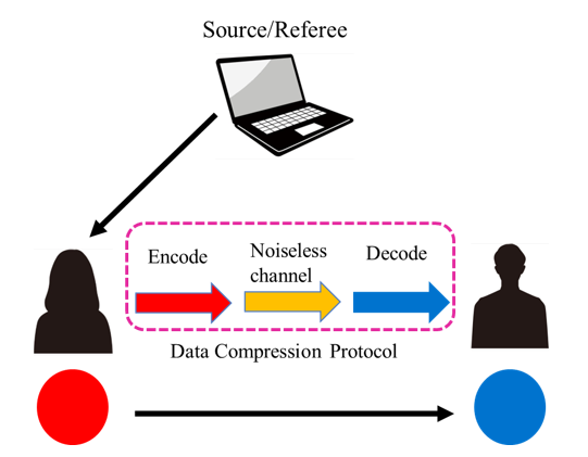
We provide a more formal description below. Suppose that $\{p_{x},\rho_{x}\}_{x\in\Sigma}$ is a quantum ensemble on system $A$. A referee draws $x\in\Sigma$ with probability $p_{x}$, writes down the outcome in a system $X$ (a classical system) with Hilbert space $\mathcal{H}_{X}\coloneqq\mathbb{C}^{\Sigma}$, and prepares $\rho_{x}$ in system $A$. The resulting state is given by $\rho_{XA}\coloneqq\sum_{x\in\Sigma}p_{x}\ket{x}\bra{x}\otimes\rho_{x}$. Note that $\rho_{A}=\sum_{x\in\Sigma}p_{x}\rho_{x}$ is the average state of the ensemble. If the referee repeats the above process $n$ times independently, then the resulting state is

where $|x_{i}\rangle\langle x_{i}|$ is a state on $X_{i}$ and $\rho_{x_{i}}$ is a state on $A_{i}$. We use the shorthand $x^{n}$ for $x_{1}x_{2}\cdots x_{n}$, $p_{x^{n}}$ for $p_{x_{1}}p_{x_{2}}\cdots p_{x_{n}}$ and $\rho_{x^{n}}$ for $\rho_{x_{1}}\otimes\rho_{x_{2}}\otimes\cdots\otimes\rho_{x_{n}}$, and $\rho_{X^{n}A^{n}}$ for $\rho_{X_{1}A_{1}}\otimes\rho_{X_{2}A_{2}}\otimes\cdots\otimes\rho_{X_{n}A_{n}}$. Then, the referee gives the systems $A_{1}A_{2}\cdots A_{n}$ to the sender. After receiving $A_{1}\cdots A_{n}$ from the referee, the sender applies to them an encoding channel $\mathcal{E}_{n}\in\mathrm{C}(\otimes_{i=1}^{n}\mathcal{H}_{A_{i}},\mathcal{H}_{M_{n}})$. When the assistance of entanglement is allowed, the sender jointly encodes $A_{1}\cdots A_{n}$ with her share of a given entangled state. Afterward, the sender transmits the system $M_{n}$ to the receiver through a noiseless quantum channel. The receiver decompresses the state by a decoding channel $\mathcal{D}_{n}\in\mathrm{C}(\mathcal{H}_{M_{n}},\otimes_{i=1}^{n}\mathcal{H}_{A^{\prime}_{i}})$, where $A^{\prime}_{i}\simeq A_{i}$ for all $i$. The final state $\id_{\mathcal{H}_{X}}^{\otimes n}\otimes(\mathcal{D}_{n}\circ\mathcal{E}_{n})(\rho_{X^{n}A^{n}})$ has to resemble the initial state $\rho_{X^{n}A^{n}}$ in a certain way. The compression protocol is defined as a pair $(\mathcal{E}_{n},\mathcal{D}_{n})$ of the encoding and decoding channels, but we also refer to their combined effect $\mathcal{D}_{n}\circ\mathcal{E}_{n}$ as the protocol.

The compression rate $R_{n}$ of the protocol is given by the number of qubits transmitted divided by $n$:

In the basic setup shown above, the protocol and compression rate depend crucially on the following:

1. 1.

   whether the given ensemble consists of pure states or mixed states;

2. 2.

   whether the referee tells the sender the label of the state to be compressed;

3. 3.

   what error criterion we adopt between the original state and the one recovered by the receiver.

In the second point mentioned above, if the sender knows the label, the task is called visible compression; otherwise, the task is called blind compression. By definition, a blind compression protocol also works in the visible setting. Correspondingly, the compression rate in the blind setting is no less than that in the visible setting. On the third point, two definitions of error criteria have been considered: global error criterion and local error criterion. Under the global error criterion, a protocol satisfying

is said to have global error $\epsilon_{n}$. In this case, the entire state emerges close to the entire original state. On the other hand, under the local error criterion, a protocol satisfying

for all integers $1\leq k\leq n$ is said to have local error $\epsilon_{n}$. In this case, the initial and final states should be close letter-wisely. In these definitions, $\tr_{\bar{(\cdot)}_{k}}$ denotes the partial trace over all systems other than the $k$th one. The global error criterion implies the local error criterion, but the converse does not always hold.

We consider an asymptotic scenario where the number $n$ of states is sufficiently large. We call a pair $(\mathcal{E}_{n},\mathcal{D}_{n})$ with an encoding channel $\mathcal{E}_{n}$ and a decoding channel $\mathcal{D}_{n}$ an $(n,R_{n},\epsilon_{n})$ code if the protocol $\mathcal{D}_{n}\circ\mathcal{E}_{n}$ yields the rate $R_{n}$ within error $\epsilon_{n}$ under the error criterion we adopt. Then, we say that the rate $R$ is achievable if for any $\epsilon>0$ and $\delta>0$, there exists a positive integer $n_{0}$ such that for all integers $n\geq n_{0}$, we can construct an $(n,R+\delta,\epsilon)$ code. Similarly, we say that the rate $R$ is achievable within error $\epsilon$ if for any $\delta>0$, there exists a positive integer $n_{0}$ such that for all integers $n\geq n_{0}$, we can construct an $(n,R+\delta,\epsilon)$ code.

Next, we will summarize the state-of-the-art understanding of quantum data compression in these setups. Quantum data compression was first studied in Refs. Schumacher 1995; Jozsa and Schumacher 1994; Barnum et al. 1996. These ground-breaking work focused on blind compression of pure-state ensembles under global error criterion. It was shown that the optimal compression rate is the quantum entropy of the average state of the given pure-state ensemble; that is, letting $\{p_{a},\ket{\psi_{a}}\}_{a\in\Sigma}$ denote a given ensemble, the optimal rate is given by the entropy of the average state,

A particularly important compression protocol, named after its inventor as Schumacher compression, was proposed in Ref. Schumacher 1995 and reviewed in various textbooks such as Refs. Nielsen and Chuang 2010; Wilde 2017; Watrous 2018.

After the aforementioned initial studies of blind compression of pure states, visible compression was subsequently considered. For a given quantum ensemble $\Phi=\{p_{a},\rho_{a}\}_{a\in\Sigma}$, which is not necessarily pure, the optimal rate is lower-bounded by the Holevo information Horodecki 1998; Barnum et al. 2001 defined as

Observe that for a pure-state ensemble, the Holevo information is equal to the entropy of the average state since the entropy of a pure state is zero. Therefore, the optimal rate of the visible compression of a pure-state ensemble is also the entropy of the average state. Thus, surprisingly, for compression of a pure-state ensemble under the global error criterion, whether the compression is visible or blind does not make any difference to the optimal rate.

After the extensive investigation of compression of pure-state ensembles, compression of general mixed-state ensemble became of central interest. Historically, the optimal rate of visible compression is called the effective information; that of blind compression is called the passive information. Letting $I_{e}(\Phi)$ denote the effective information of a quantum ensemble $\Phi$ and $I_{p}(\Phi)$ denote the passive information of a quantum ensemble $\Phi$, we have the following relation:

since visible compression can be regarded as a subclass of blind compression. The quantity $I_{d}\coloneqq I_{p}-I_{e}$ is called the information defect, and it characterizes a difference between the visible and blind compression tasks. In Ref. Horodecki 1998; Barnum et al. 2001, a lower bound of the information defect was given, and Refs. Dür et al. 2001; Kramer and Savari 2001 showed examples for which the information defect is strictly positive. Moreover, the optimal rate of visible compression was derived in Ref. Horodecki 2000, and the optimal rate is given by the entropy of an extension of a given state. In Ref. Hayashi 2006, the authors gave another representation of the optimal rate of the visible compression. On the other hand, in Ref. Koashi and Imoto 2001, the optimal rate of blind compression was studied. The main difficulty of blind compression is that the sender does not know the label of a given state. The authors proposed a protocol in which the sender only sends the essential parts of a given ensemble, and the compression rate achieved by the protocol is given by the KI decomposition Koashi and Imoto 2002. This optimal protocol is based on a block coding of mixed states proposed in Ref. Lo 1995. In fact, this compression rate is optimal under both the global and local error criteria.

Here, let us note that we mainly discuss quantum data compression without any assistance; however, data compression tasks with assistance, e.g., entanglement and shared randomness, have also been widely investigated Bennett et al. 2001; Bennett et al. 2005; Abeyesinghe et al. 2006; Jain et al. 2002; Bennett et al. 2014; Anshu et al. 2022; Khanian and Winter 2020

Blind data compression is a quantum information processing task between two parties, the sender and the receiver, in which fundamental quantum properties emerge. As also mentioned in Sec. II.3, in blind data compression, the sender aims to asymptotically send quantum data without knowing its actual description to the receiver as efficiently as possible.

Here we describe a formal procedure of blind quantum data compression following the setup shown in Sec. II.3. Let $\{p_{x},\rho_{x}\}_{x\in\Sigma}$ be a quantum ensemble the sender wants to send. The referee draws a state from the ensemble $n$ times in an independent and identically distributed (i.i.d.) manner, and let the resulting $n$-fold state be denoted by $\rho_{x^{n}}$. Then, the referee gives the state $\rho_{x^{n}}$ to the sender. What is crucial in this setup is that the referee does not tell the sender the label $x^{n}$ of the state. After receiving the state $\rho_{x^{n}}$ from the referee, the sender encodes the state by an encoding channel $\mathcal{E}_{n}$ and transmits the compressed state to the receiver through a noiseless quantum channel. The receiver decompresses the state by a decoding channel $\mathcal{D}_{n}$ to recover the initial state $\rho_{x_{n}}$. Note that they do not know the description of the given state while the sender has knowledge about the ensemble. Therefore, the compression scheme $(\mathcal{E}_{n},\mathcal{D}_{n})$ cannot be state-specific and must only depend on the ensemble.

Now, we provide an overview of the achievable rates of blind data compression. In Ref. Lo 1995, an achievable rate of blind state compression with a mixed state ensemble was investigated. It was figured out that the quantum entropy of the average state is an achievable rate even for a mixed state ensemble; that is, for a given ensemble $\{p_{x},\rho_{x}\}_{x\in\Sigma}$,

is achievable. It had been open whether this rate is optimal or not Lo 1995; Horodecki 1998; Barnum et al. 2001; Dür et al. 2001; Kramer and Savari 2001 before Ref. Koashi and Imoto 2001 conducted a more detailed analysis.

In Ref. Koashi and Imoto 2001, the authors applied the Koashi-Imoto(KI) decomposition (Theorem 3 in Sec. II.2) to derive the optimal rate of blind compression. Recall that when an ensemble $\{p_{x},\rho_{x}\}_{x}$ is given, we have the KI decomposition

Then, as shown in Theorem 4, we can define quantum channels $\mathcal{K}_{\mathrm{off}}$ and $\mathcal{K}_{\mathrm{on}}$ satisfying

for all $x\in\Sigma$. With these operations, the sender does not necessarily send the redundant parts of a target ensemble if the sender and the receiver agree on the ensemble in the scenario of blind data compression. If they both know the description of the ensemble, they also agree on $\mathcal{K}_{\mathrm{off}}$ and $\mathcal{K}_{\mathrm{on}}$; that is, they can freely take off and put on the redundant parts. Therefore, the sender only needs to send the classical and non-redundant quantum parts. By applying the argument of Ref. Lo 1995 after removing the redundant parts, we obtain an achievable rate

In addition, Ref. Koashi and Imoto 2001 also proved that Eq. (26) is optimal even under local error criterion. To summarize, we have the following theorem.

To show the optimality of the rate, the authors of Ref. Koashi and Imoto 2001 introduced two error functions of compression protocol $\Lambda_{n}\coloneqq(\mathcal{E}_{n},\mathcal{D}_{n})$:

with

Here, $\fidelity(\cdot,\cdot)$ is the fidelity function, and $\rho$ is the average state of the given ensemble with the spectral decomposition

Moreover, $h_{2}(\cdot)$ is the binary entropy function defined as

for $x\in[0,1]$. It was shown that when the protocol $\Lambda_{n}$ is given, the compression rate $R$ is

The authors proved the optimality by showing that when $f(\Lambda_{n})$ goes to zero, $g(\Lambda_{n})$ also converges to zero; that is, for an infinitesimal error, $R^{*}$ is the smallest compression rate that can be achievable.

Recently, Ref. Khanian and Winter 2020 further investigated the optimality of the compression rate under the global error criterion. The authors introduced an error function that represents how an error allowed in the protocol affects the compression rate, and they revealed properties of this error function to study how the compression rate depends on an error. On the other hand, in this paper, we focus on local error criterion to investigate the sensitivity of the rate against approximations.

In this subsection, we motivate and describe our protocol for blind quantum data compression. Here, we consider local error criterion; that is, we only require the resulting state to be close to the original state letter-wisely. In addition, we allow finite approximations to the resulting state under this error criterion.

We first summarize the compression scheme from the previous section:

1. 1.

   After receiving a state $\rho_{x^{n}}$ from the referee, the sender applies $\mathcal{K}_{\mathrm{off}}$ letter-wisely to remove the redundant parts of the state and obtain $\mathcal{K}_{\mathrm{off}}^{\otimes n}(\rho_{x^{n}})$.

2. 2.

   The sender encodes the state $\mathcal{K}_{\mathrm{off}}^{\otimes n}(\rho_{x^{n}})$ using an encoding channel $\mathcal{E}_{n}$ to obtain $\mathcal{E}_{n}\circ\mathcal{K}_{\mathrm{off}}^{\otimes n}(\rho_{x^{n}})$.

3. 3.

   The sender sends the state $\mathcal{E}_{n}\circ\mathcal{K}_{\mathrm{off}}^{\otimes n}(\rho_{x^{n}})$ via a noiseless quantum channel to the receiver.

4. 4.

   The receiver decodes the transmitted state using a decoding channel $\mathcal{D}_{n}$ and obtains $\mathcal{D}_{n}\circ\mathcal{E}_{n}\circ\mathcal{K}_{\mathrm{off}}^{\otimes n}(\rho_{x^{n}})$.

5. 5.

   The receiver put the redundant parts back using the quantum channel $\mathcal{K}_{\mathrm{on}}$; the resulting state is $\mathcal{K}_{\mathrm{on}}^{\otimes n}\circ\mathcal{D}_{n}\circ\mathcal{E}_{n}\circ\mathcal{K}_{\mathrm{off}}^{\otimes n}(\rho_{x^{n}})$.

Our main idea is as follows. We may use quantum channels $\Lambda_{s}^{(n)}$ and $\Lambda_{r}^{(n)}$, potentially acting jointly on the entire state, instead of $\mathcal{K}_{\mathrm{off}}^{\otimes n}$ and $\mathcal{K}_{\mathrm{on}}^{\otimes n}$. The encoding and decoding maps $\mathcal{E}_{n}$ and $\mathcal{D}_{n}$ may change accordingly. When we allow a finite, local, approximation of the given state $\rho_{x^{n}}$ by the resulting state $\Lambda_{s}^{(n)}\circ\mathcal{D}_{n}\circ\mathcal{E}_{n}\circ\Lambda_{r}^{(n)}(\rho_{x^{n}})$, a smaller rate may be achieved than the previous optimal rate with a vanishing error. We show that even if $\Lambda_{s}^{(n)}$ and $\Lambda_{r}^{(n)}$ are letter-wise approximations, it is plausible that a reduction of the compression rate may be observed.

In our protocol, we use the KI operations of a different quantum ensemble on the given ensemble, and prove that this approximation procedure indeed performs well and reduces the rate. In more detail, suppose we are given a quantum ensemble $\{p_{x},\rho_{x}\}_{x\in\Sigma}$ and the resulting state can differ letter-wisely from the original state up to $\epsilon>0$. We consider all possible approximate ensembles $\{p_{x},\tilde{\rho}_{x}\}_{x\in\Sigma}$, such that $\tilde{\rho}_{x}$ is close to $\rho_{x}$ in the original given ensemble for each $x$. Each such approximate ensemble defines KI operations $\tilde{\mathcal{K}}_{\mathrm{off}}$ and $\tilde{\mathcal{K}}_{\mathrm{on}}$ as in Theorem 4. Now, suppose we use these KI operations $\tilde{\mathcal{K}}_{\mathrm{off}}^{\otimes n}$ and $\tilde{\mathcal{K}}_{\mathrm{on}}^{\otimes n}$ as an approximation scheme $\Lambda_{s}^{(n)}$ and $\Lambda_{r}^{(n)}$ for $\{p_{x},\rho_{x}\}_{x\in\Sigma}$. How much error do we incur? If the error is small, what rate can be achieved? Before we answer these questions, let us formally define our compression protocol with local approximations.

• 0.

  The sender and receiver pre-agree on an approximate ensemble $\{p_{x},\tilde{\rho}_{x}\}_{x\in\Sigma}$ of the original given ensemble $\{p_{x},\rho_{x}\}_{x\in\Sigma}$ such that for all $x\in\Sigma$,

  $$~\left\|\;\tilde{\mathcal{K}}_{\mathrm{on}}\circ\tilde{\mathcal{K}}_{\mathrm{off}}(\rho_{x})-\rho_{x}\;\right\|_{1}\leq\epsilon\,,$$

  (39)

• 1.

  The referee gives a state $\rho_{x^{n}}$ generated by $n$ independent and identically distributed (i.i.d.) draws from $\{p_{x},\rho_{x}\}_{x\in\Sigma}$ to the sender. The sender applies $\tilde{\mathcal{K}}_{\mathrm{off}}^{\otimes n}$ to the given state, which yields $\tilde{\mathcal{K}}_{\mathrm{off}}^{\otimes n}(\rho_{x^{n}})$.

• 2.

  The sender applies an encoding operation $\mathcal{E}_{n}$ to obtain $\mathcal{E}_{n}\circ\tilde{\mathcal{K}}_{\mathrm{off}}^{\otimes n}(\rho_{x^{n}})$.

• 3.

  The sender transmits the encoded state $\mathcal{E}_{n}\circ\tilde{\mathcal{K}}_{\mathrm{off}}^{\otimes n}(\rho_{x^{n}})$ to the receiver via a noiseless quantum channel.

• 4.

  Upon receiving the state, the receiver applies the decoding channel $\mathcal{D}_{n}$ corresponding to $\mathcal{E}_{n}$, which yields $\mathcal{D}_{n}\circ\mathcal{E}_{n}\circ\tilde{\mathcal{K}}_{\mathrm{off}}^{\otimes n}(\rho_{x^{n}})$.

• 5.

  Finally, the receiver applies $\tilde{\mathcal{K}}_{\mathrm{on}}^{\otimes n}$ to obtain the resulting state $\tilde{\mathcal{K}}_{\mathrm{on}}^{\otimes n}\circ\mathcal{D}_{n}\circ\mathcal{E}_{n}\circ\tilde{\mathcal{K}}_{\mathrm{off}}^{\otimes n}(\rho_{x^{n}})$.

The resulting state $\tilde{\mathcal{K}}_{\mathrm{on}}^{\otimes n}\circ\mathcal{D}_{n}\circ\mathcal{E}_{n}\circ\tilde{\mathcal{K}}_{\mathrm{off}}^{\otimes n}(\rho_{x^{n}})$ of our protocol should be close to the original state $\rho_{x^{n}}$. In step 2 of the protocol, we choose $\mathcal{E}_{n}$ to achieve blind compression of the ensemble $\{p_{x},\tilde{\mathcal{K}}_{\mathrm{off}}(\rho_{x})\}_{x\in\Sigma}$ with vanishing error. That is, for any $\delta>0$, there exists a positive integer $n_{0}$ such that for all integers $n\geq n_{0}$,

Together with condition (39), local error will be $\leq\epsilon+\delta$. In the rest of the paper, we omit $\delta$ considering that we may take $\delta$ arbitrarily small by choosing $n$ appropriately.

In our protocol, the condition (39) is crucial. Here, we give a sufficient condition for Eq. (39); we prove that $\tilde{\mathcal{K}}_{\mathrm{off}}$ and $\tilde{\mathcal{K}}_{\mathrm{on}}$ satisfy the local error criterion for $\{p_{x},\rho_{x}\}_{x\in\Sigma}$ if $\{p_{x},\tilde{\rho}_{x}\}_{x\in\Sigma}$ is close enough to the original ensemble. Suppose that $\{p_{x},\rho_{x}\}_{x\in\Sigma}$ is a quantum ensemble, and let $\{p_{x},\tilde{\rho}_{x}\}_{x\in\Sigma}$ be a quantum ensemble such that

for all $x$. Then,

The second line follows from the triangle inequality. In the third line, we used the monotonicity of the trace norm and the relation $\tilde{\mathcal{K}}_{\mathrm{on}}\circ\tilde{\mathcal{K}}_{\mathrm{off}}(\tilde{\rho}_{x})=\tilde{\rho}_{x}$. Thus,

that is, a quantum ensemble for which each state is $\epsilon/2$-close to the state in the original ensemble works as an approximate ensemble for our protocol.

Second, we analyze the rate performance of our protocol. The compression rate of our protocol is determined by $\mathcal{E}_{n}$; a rate of

is sufficient to ensure vanishing error condition (40). In step 0 of the protocol, the sender and the receiver can minimize the above rate by optimizing the approximate ensemble:

In this protocol, we need to find a good approximate ensemble to reduce the compression rate. While this optimization may not be intractable, it suffices to find good enough approximate ensemble to substantially reduce the rate, as we will see in the next section.

Here, we present two main examples for which our protocol performs better than the case where finite approximations are not allowed. The first example is over a small dimensional system, and it illustrates the procedure and performance of our protocol in an intuitive way; the second example is over a growing dimension, and exhibits a growing reduction of the compression rate.

First, we consider a four-dimensional two-state ensemble to intuitively understand the protocol.

Next, we show an example for which a finite approximation dramatically changes the KI structure of a given ensemble. For this example, we can see a large reduction of the compression rate compared with the compression rate under asymptotically vanishing errors.