Recent Advances in Bayesian OptimizationCCS: General and reference Surveys and overviewsCCS: Theory of computation Bayesian analysisCCS: Mathematics of computing Nonparametric statistics
Abstract.
Bayesian optimization has emerged at the forefront of expensive black-box optimization due to its data efficiency. Recent years have witnessed a proliferation of studies on the development of new Bayesian optimization algorithms and their applications. Hence, this paper attempts to provide a comprehensive and updated survey of recent advances in Bayesian optimization and identify interesting open problems. We categorize the existing work on Bayesian optimization into nine main groups according to the motivations and focus of the proposed algorithms. For each category, we present the main advances with respect to the construction of surrogate models and adaptation of the acquisition functions. Finally, we discuss the open questions and suggest promising future research directions, in particular with regard to heterogeneity, privacy preservation, and fairness in distributed and federated optimization systems.
Keywords:
Bayesian optimization, Gaussian process, acquisition function1. Introduction
Optimization problems are pervasive in scientific and industrial fields, such as artificial intelligence, data mining, bioinformatics, software engineering, scheduling, manufacturing, and economics. Among them, many applications require to optimize objective functions that are noisy and expensive to evaluate, or do not have closed-form expressions, let alone gradient information. For such problems, metaheuristics such as evolutionary algorithms that rely on function values only are very popular. However, these algorithms usually require a large number of function evaluations. By contrast, Bayesian optimization has emerged as a mainstream to tackle these difficulties due to its high data efficiency, thanks to its ability to incorporate prior beliefs about the problem to help guide the sampling of new data, and to achieve a good balance between exploration and exploitation in the search.
Consider the maximization of an unknown function that is expensive to evaluate, which can be formulated as follows:
| (1) |
where denotes the search/decision space of interest and is the global maximum. In principle, Bayesian optimization constructs a probabilistic model (also known as a surrogate model) that defines a distribution over the objective function, and then subsequently refines this model once new data is sampled. Specifically, Bayesian optimization first specifies a prior distribution over the function, which represents our belief about the objective function. Then, conditioned on the observed data and the prior, the posterior can be calculated using the Bayes rule, which quantifies our updated belief about the unknown objective function. As a result, the next sample can be identified by leveraging the posterior. This is achieved by optimizing some auxiliary functions, called acquisition functions in Bayesian optimization.
The origin of Bayesian optimization can be dated back to the work by Harold Kushner (Kushner 1964), where Wiener processes were adopted for unconstrained one-dimensional optimization problems and the probability of improvement is maximized to select the next sample. Mockus (Močkus 1975) developed a new acquisition function, called expectation of improvement (EI), which was further used in (Zilinskas et al. 1978). Stuckman (Stuckman 1988), Perttunen (Perttunen and Stuckman 1990) and Elder (Elder 1992) extended Kushner’s work to high-dimensional problems. Bayesian optimization was made popular in engineering after Jones et al. (Jones et al. 1998) introduced Efficient Global Optimization (EGO). In EGO, a Kriging model, called Design and Analysis of Computer Experiments (DACE) stochastic process model (Sacks et al. 1989), is adopted to provide best linear unbiased predictions of the objective, which is achieved by minimizing the Mean Squared Error of the predictor (Kleijnen 2009). In Bayesian optimization, by contrast, a Gaussian process is adopted as the surrogate model, which is fit by maximizing the likelihood. Hence, the original formulation of Kriging is different from the Gaussian process (Cressie 1990). More recently, various variants of Kriging have been developed (Van Beers and Kleijnen 2003; Huang et al. 2006b) by accounting for constraints and noise in the optimization. As a result, Kriging models in spatial statistics are equivalent to Gaussian processes in Bayesian optimization in some papers, therefore the two terms will be used interchangeably in the rest of this paper. The past decades have witnessed a rapid development of Bayesian optimization in many real-world problems, including materials design and discovery (Frazier and Wang 2016), sensor network (Garnett et al. 2010), financial industry (Gonzalvez et al. 2019), and experimental design (Lorenz et al. 2019). More recently, Bayesian optimization became popular in machine learning, including reinforcement learning (Turchetta et al. 2020), hyperparameter tuning (Wu et al. 2020), and neural architecture search (Kandasamy et al. 2018b).
1.1. Related Surveys
There are already a few comprehensive surveys and tutorials on methodological and practical aspects of Bayesian optimization, each with a specific focus. Sasena (Sasena 2002) gave a review of early work on Kriging and its extension to constrained optimization. A tutorial on Bayesian optimization with Gaussian processes was given in (Brochu et al. 2010), focusing on extending Bayesian optimization to active user modelling in preference galleries and hierarchical control problems. Shahriari et al. (Shahriari et al. 2016) presented a comprehensive review of the fundamentals of Bayesian optimization, elaborating on the statistical modeling and popular acquisition functions. In addition, Frazier (Frazier 2018) discussed some recent advances in Bayesian optimization, in particular in multi-fidelity optimization and constrained optimization.
However, none of the above review papers provides a comprehensive coverage of abundant extensions of Bayesian optimization. Moreover, many new advances in Bayesian optimization have been published since (Shahriari et al. 2016). Hence, an updated and comprehensive survey of this dynamic research field will be beneficial for researchers and practitioners.
1.2. Contributions and Organization

This paper starts with a brief introduction to the fundamentals of Bayesian optimization in Section 2, including Gaussian processes and commonly used acquisition functions. Section 3 provides a comprehensive review of the state-of-the-art, where a taxonomy of existing work on Bayesian optimization is proposed to offer a clear structure of the large body of research reported in the literature, as illustrated in Fig. 1. In this taxonomy, existing Bayesian optimization algorithms are divided into nine groups according to the nature of the optimization problems. We further introduce a color-coding scheme to highlight the focuses of each group, where red, blue and yellow blocks indicate, respectively, a focus on acquisition functions, surrogates, or both. Finally, this survey explores a few emerging topics in Bayesian optimization, including Bayesian dynamic optimization, distributed and federated Bayesian optimization, and heterogeneity and fairness in optimization.
2. Fundamentals of Bayesian Optimization
Gaussian processes and acquisition functions are two main components of Bayesian optimization, which are introduced in the following.
2.1. Gaussian Process
Gaussian process (GP) is the most widely used probabilistic surrogate model for approximating the true objective function in Bayesian optimization. GP is characterized by a prior mean function and a covariance function (Rasmussen 2003). Consider a finite collection of data pairs of the unknown function with noise , where is the input and is the output resulting from the true objective evaluations, and is the number of samples. The Gaussian process model assumes that the observed data are drawn from a multivariate Gaussian distribution. Therefore, for a new data point , the joint distribution of the observed outputs and the predicted output are
| (2) |
where denotes matrix transposition, denotes an correlation matrix, and denotes a correlation vector evaluated at all pairs of training and test points. As described in (Rasmussen 2003), the conditional distribution is then a multivariate Gaussian distribution, where the mean and variance of the predicted output can be estimated as
| (3) | ||||
Commonly used kernel functions are the squared exponential (Gaussian) kernel and the Matáern kernel (Frazier 2018), where hyperparameters, such as length scale, signal variance, and noise variance need to be specified. Typically, the optimal hyperparameters are inferred by maximizing the log marginal likelihood,
| (4) |
where .
2.2. Acquisition Function
BO starts by sampling a training set from the black-box function, by which a Gaussian process is constructed. At each iteration, an acquisition function is evaluated based the GP and optimised to identify where to sample next (green point) from the true objective function. The new sample is added into the training set to update the model. This procedure is repeated until until the termination condition is met.
Acquisition functions (AFs) are the utility functions that guide the search to reach the optimum of the objective function by identifying where to sample next, which is crucial in Bayesian optimization. The guiding principle behind AFs is to strike a balance between exploration and exploitation, which is achieved by querying samples from both known high-fitness-value regions and regions that have not been sufficiently explored so far. While the top row in each panel shows a Gaussian process, the lower four rows illustrate four commonly used AFs. In the following, we briefly revisit the commonly used AFs.
Without loss of generality, we consider a maximization problem. Let denote the optimum obtained so far, and and denote the normal cumulative distribution function (CDF), and probability density function (PDF) of the standard normal random variable, respectively. The earliest acquisition function is to maximize the probability of improvement (PI) (Kushner 1964) over the current best value , formulated as
| (5) |
where is the probability for finding a better objective function value at position than the currently best value , which, for a Gaussian process, is given by the Gaussian cumulative distribution function (CDF) .
Alternatively, expected improvement (EI) (Močkus 1975) calculates the expected improvement with respect to ,
| (6) | ||||
where denotes the expectation value, and are the Gaussian CDF and PDF, respectively. EI dates back to 1975 (Močkus 1975) and was popularized by Jones et al. (Jones et al. 1998). A wealth of research has been dedicated to the development of EI in various applications, including parallel optimization, multi-objective optimization, constrained optimization, noisy optimization, multi-fidelity optimization, and high-dimensional optimization.
Interested readers are referred to (Zhan and Xing 2020) for a comprehensive review of many variants of EI. Note, however, that EI tends to explore around the initial best point before the algorithm begins to search more globally, as only points that are close to the current best point have high EI values.
An idea closely related to EI is Knowledge Gradient (KG) (Frazier et al. 2008), maximizing the expected incremental value of a measurement; however, it does not depend on the optimum obtained so far. Let denote the mean of the posterior distribution after samples, and a new posterior distribution with posterior mean will be generated if we take one more sample. Hence, the KG is formulated as
| (7) |
where indicates the conditional expectation with respect to what is known after the first measurements.
The confidence bound criteria, upper confidence bound (UCB) for maximization problems and lower confidence bound (LCB) for minimization problems, are designed to achieve optimal regret in the multi-armed bandit community by combining the uncertainty and the expected reward (Srinivas et al. 2009). The UCB is calculated as
| (8) |
where is a parameter to navigate the exploitation-exploration trade-off (LCB has a minus sign in front of the term). A recent work (De Ath et al. 2021b) presents -greedy acquisition functions, where the location with the most promising mean prediction is usually selected, while a multi-objective optimiser is used to generate the Pareto-optimal solutions in the remaining cases.
Another promising acquisition function for multi-armed bandit problems is Thompson sampling (TS) (Agrawal and Goyal 2012). TS randomly draws each arm sampled from the posterior distribution, and then plays the arm with the highest simulated reward (Russo et al. 2017). More recently, TS has seen a surge of interests spurred by the fact that TS can be fully parallelized and distributed (Hernández-Lobato et al. 2017; Garcia-Barcos and Martinez-Cantin 2019; Dai et al. 2020; Kandasamy et al. 2018a).
A more recent development is the entropy-based AFs motivated by information theory, which can be further divided into input-entropy-based and output-entropy-based AFs. The former maximizes information about the location of the global optimum where the information about is measured by the negative differential entropy of the probability of the location of the global optimum, (Hennig and Schuler 2012; Hernández-Lobato et al. 2014). Hennig and Schuler (Hennig and Schuler 2012) proposed entropy search (ES) using mutual information ,
| (9) | ||||
where denotes the differential entropy and denotes the expectation over a probability distribution . However, the calculation in Eq. (9) is computationally intractable. To resolve this problem, Lobato et al. introduced predictive entropy search (PES) by equivalently rewriting Eq. (9) as
| (10) |
Compared with the previous formulation, PES is based on the entropy of predictive distributions, which is analytic or can be easily approximated. Following the same information-theoretic idea, output-entropy-based AFs maximize the reduction of the information about the maximum function value , the mutual information instead (Wang and Jegelka 2017). The max-value entropy search (MES) is formulated as
| (11) | ||||
Intuitively, MES is computationally much simpler than ES and PES as MES uses one-dimensional while ES and PES estimate the expensive and multidimensional . Empirical results have demonstrated that MES performs at least as good as ES and PES.
Note that the above mentioned AFs are all designed for single-objective optimization, and therefore, many recent efforts have been dedicated to developing more new AFs to account for a diverse and wide range of applications.
3. Recent Advances in Bayesian Optimization
In the above we provided a brief history of Bayesian optimization, and described the methodology for solving the standard Bayesian optimization problem, i.e., black-box single-objective optimization. In this section, we provide an overview of the state-of-the-art Bayesian optimization algorithms, focusing on the most important research advances. In the following, we categorize and discuss the existing work according to the characteristics of the optimization problems to provide a clear picture of the abundant literature.
3.1. High-dimensional optimization
High-dimensional black-box optimization problems are extremely challenging yet commonly seen in many applications (Wang et al. 2018; Nayebi et al. 2019). For example, in hyperparameter optimization of machine learning models (Ranjit et al. 2019), the number of hyperparameters and the size of search space grow as the complexity of the models increases. Despite successful applications of Bayesian optimization to low-dimensional expensive and black-box optimization problems, its extension to high-dimensional problems remains a critical open challenge. The dimension of the search space impacts both the construction of GPs and the optimization of AFs. Specifically, the following major difficulties can be identified for Bayesian optimization of high-dimensional problems. 1) Nonparametric regression, such as the GP model, is inherently difficult as the search space grows exponentially with the dimension. On the one hand, it becomes harder to learn a model in a high-dimensional space with the commonly used distance-based kernel functions, as the search spaces grow considerably faster than affordable sampling budgets. On the other hand, the number of hyperparameters generally increases along with the input dimension, as a consequence, the training of the model becomes increasingly hard. 2) Generally, AFs are multi-modal problems, with a large mostly flat surface. Hence, the optimization of AFs is non-trivial, in particular for high-dimensional problems and when the number of samples is limited. For example, Tian et al. (Tian et al. 2019) observed that the estimated uncertainty of different solutions in high-dimensional spaces are very similar, reducing the effectiveness of acquisitions based on the estimated uncertainty. Hence, a bi-objective acquisition function was proposed, which is solved using a multi-objective evolutionary algorithm (Zhou et al. 2011). The reader is referred to Section 3.5 for a more detailed discussion on multi-objective evolutionary algorithms (MOEAs).
Also, our focus is primarily on the surrogate modeling techniques themselves, not the experimental designs used to generate sample data; interested readers are referred to recent overviews and texts on the topic the GPs are subjected to the scalability challenge In view of the space limit and the fact that some of strategies are studied in special areas (e.g., parallel computing and increasing computer power), this section only reviews some of them that directly deal with high-dimensionality. Note that the above problem is related to, but distinct from the scalability of GPs. To construct a reliable GP in higher dimensional space, more observed data may be required, which results in a challenge of scalability for the GP due to its cubic complexity to the data size. Although scalable GPs have been extensively studied in recent years to accommodate many observations (Liu et al. 2020), these methods focus on the scenario where there exist a large amount of data while the dimension remains to be small or medium. Moreover, even if one can fit a GP model for high-dimensional problems, one would still face the difficulty of the optimization of acquisition functions. Therefore, we are interested in scalable Bayesian optimization algorithms for tackling high dimensionality, rather than construction of high-dimensional GPs only.
Most existing Bayesian optimization algorithms for high-dimensional problems make two structural assumptions, namely low active/effective dimensionality of the objective function together with an additive structure with few exceptions (Eriksson and Jankowiak 2021). Addressing high-dimensional Bayesian optimization with a large amount data generally involves alternative models, local modelling, and batch selection in a parallel manner. In the following, we will discuss in detail existing work handling high-dimensional optimization problems. A comprehensive survey paper in this line can be found in (Binois and Wycoff 2021), in which the high-dimensional GP modeling is introduced before presenting its application to BO.
3.1.1. Variable selection
To alleviate the curse of dimensionality, a straightforward idea is to adopt a dimension reduction technique. To achieve this, an important assumption often made is that the original objective function varies only within a low-dimensional subspace, called active/effective subspace (Chen et al. 2012). To identify the most contributing input variables, some sensitivity analysis techniques that evaluate the relative importance of each variable with respect to a quantity of interest have been exploited (Spagnol et al. 2019). In (Chen et al. 2012) two strategies, the finite difference sequential likelihood ratio test and the GP sequential likelihood ratio test, are proposed to screen the most contributing variables. Another commonly used quantity is the values of the correlation lengths of automatic relevance determination (ARD) covariances (Winkel et al. 2021). The basic idea is that the larger the length scale value, the less important the corresponding variable.
3.1.2. Linear/non-linear embedding
Instead of removing the inactive variables to reduce the dimension, more recent developments exploit the active dimensionality of the objective function by defining a latent space based on a linear or non-linear embedding. For example, Wang et al. (Wang et al. 2013) noted that given any and a random matrix , at a probability of 1, there is a point such that . This observation allows us to perform Bayesian optimization in a low-dimensional space to optimize the original high-dimensional function. Hence, an algorithm, called Bayesian optimization with random embedding (REMBO), is proposed. REMBO first randomly generates an embedding denoted as a matrix and constructs a GP model, and then optimizes an AF to select a new data point that will be projected back to the original space using inverse random projection. Some studies have been dedicated to further investigate the random embedding in recent years. For example, Binois et al. (Binois et al. 2020) defined a linear embedding by inverting the orthogonal projection to relax the bounded region of the embedding in REMBO. Similar to (Binois et al. 2020), matrix is used to project the ambient space down to the embedding in (Letham et al. 2020). Moreover, the authors gave the reader further insights into the linear embedding for Bayesian optimization in terms of crucial issues and misconceptions, and consequently proposed an adaptive linear embedding Bayesian optimization algorithm. In addition, Nayebi et al. (Nayebi et al. 2019) developed an inverse embedding based on a hashing function, and Bayesian optimization with the proposed embedding in combination of a set of AFs has been investigated. Inspired by the studies in (Wang et al. 2013), Cartis et al. (Cartis and Otemissov 2020; Cartis et al. 2021) extend REMBO to affine subspaces.
Apart from the success in the random embedding methods, many algorithms have been proposed to learn the intrinsic effective subspaces, such as unsupervised learning based on variational auto-encoders (Antonova et al. 2020), supervised learning (Zhang et al. 2019), and semi-supervised learning (Siivola et al. 2021). Specifically, unsupervised dimensionality reduction in the context of high-dimensional Bayesian optimization includes principal component analysis and variational auto-encoders (VAEs). Note that VAEs have emerged as a powerful method for mapping the high-dimensional input space to a low-dimensional latent space. Hence, some research resorts to VAEs to alleviate the scalability issue of Bayesian optimization in high-dimensional input spaces. The early studies for VAE-based Bayesian optimization learn the latent space in an unsupervised way (Antonova et al. 2020). The disadvantage of such a latent space learned using unlabeled data only might be sub-optimal for the optimization task. To address this problem, the most recent work has jointly learned the latent space based on label guidance in a semi-supervised way (Siivola et al. 2021). On the other hand, Zhang et al. (Zhang et al. 2019) presented a supervised dimension reduction method, sliced inverse regression (SIR), for high-dimensional Bayesian optimization (SIR-BO). SIR-BO performs a heuristic algorithm, i.e., CMA-ES, on the original search space and to optimize the UCB. Alternatively, in (Moriconi et al. 2020) two mappings, a non-linear feature mapping to reduce the dimensionality of inputs and a reconstruction mapping to evaluate the objective function, are learned in a supervised learning manner. Consequently, the AF can be optimized in the lower-dimensional feature space. In (Chen et al. 2020), an extension of SIR using semi-supervised discriminant analysis is proposed, called semi-SIR, to incorporate both labeled and unlabeled points acquired from the acquisition function of Bayesian optimization to learn the embedding space.
Most of the above-mentioned methods based on the structural assumption use linear projections to scale Bayesian optimization to high dimensions. Recently, a few advanced techniques have been developed to further investigate the structure of the search space by using non-linear embeddings. Compared with linear embeddings, non-linear embedding techniques, also known as geometry-aware Bayesian optimization (Oh et al. 2018), can be considerably more expressive and flexible. However, these methods require even more data to learn the embedding and assume that the search space is not Euclidean but various manifolds, such as Riemannian manifold (Jaquier et al. 2019). The Euclidean geometry of the search space incurs the boundary issue where an algorithm over-explores the boundaries of the search space, especially in high dimensions. Under this observation, Oh et al. (Oh et al. 2018) applied a cylindrical geometric transformation on the search space, resulting in a new kernel, referred to as the cylindrical kernel. By leveraging the new kernel in Bayesian optimization, called BOCK, one can easily scale it to more than 50 dimensions and mitigate the boundary issue. Arguably, BOCK is the first work where geometry-awareness is considered within the framework of Bayesian optimization.
Another seminal avenue is built on Riemannian manifold theory. For applications with non-Euclidean search spaces, such as robotics (Jaquier et al. 2019), the Euclidean methods can be quite brittle, motivating the recently developed geometry-aware Bayesian optimization. Geometry-awareness is introduced into Bayesian optimization to exploit the manifold’s geometric structure, so that the GP can properly measure the similarities of the non-Euclidean parameter space, with the hope of improving Bayesian optimization’s performance and scalability. To achieve this, Jaquier et al. (Jaquier et al. 2019) proposed a geometry-aware Bayesian optimization (GaBO) with new kernels measuring the similarities of manifold-valued data, and two commonly used manifolds in robotics have been considered, i.e., the sphere and symmetric positive definite manifolds. Moreover, the optimization of AFs is performed on Riemannian manifolds. A subsequent work by Jaquier and Rozo (Jaquier and Rozo 2020) extends GaBO to high-dimensional problems, namely HD-GaBO, by learning a nested structure-preserving mapping from the original manifold to a lower-dimensional latent space. In HD-GaBO, the mapping and the objective function in the latent space are jointly learned using a manifold Gaussian process (mGP) with the geometry-aware kernel function. It is necessary to investigate mathematical theory and techniques for building new kernels in the manifold settings, since the naive geometric approximations may lead to ill-defined kernels. To address this problem, Borovitskiy et al. (Borovitskiy et al. 2020) provided mathematically sound techniques for computing the geometry-aware kernels in the Riemannian setting via Laplace–Beltrami eigenfunctions. The most recent work by Jaquier et al. (Jaquier et al. 2021) has extend the GaBO with the theoretically-grounded Matérn kernels proposed in (Borovitskiy et al. 2020) in robotics.
3.1.3. Addictive structure
The low active dimensionality assumption behind the aforementioned methods is too restrictive as all the input variables may contribute to the objective function. Hence, another salient structure assumption, called addictive structure, has been explored in the context of high-dimensional Bayesian optimization. Note that the addictive structure has been widely used in addictive models (Lin and Roshan Joseph 2020; Chen and Tuo 2020) and kernel functions. A prominent work in the context of Bayesian optimization and bandits, namely Add-GP-UCB, was proposed in (Kandasamy et al. 2015), assuming that the objective function is a sum of functions of small, disjoint groups of dimensions. Instead of directly using addictive kernels, a set of latent decompositions of the feature space is generated randomly and the one with the highest GP marginal likelihood is chosen, with each kernel operating on subsets of the input dimensions. Markov Chain Monte Carlo (MCMC) (Gardner et al. 2017), Gibbs sampling (Wang et al. 2017) and Thompson sampling (Wang and Jegelka 2017) were also introduced to more effectively learn the addictive structure. A recent work by Delbridge et al. (Delbridge et al. 2020) presents a learning-free addictive GP based on sequences of multiple random projections to avoid the computationally expensive learning for the addictive structure.
Another major issue concerning Add-GP-UCB is the restriction of disjoint subsets of input dimensions, which have been lifted in subsequent work (Li et al. 2016; Rolland et al. 2018). Li et al. generalized the two structure assumptions, i.e., the low active assumption and the addictive structure assumption, by introducing a projected-addictive assumption. In (Rolland et al. 2018), overlapping groups are allowed by representing the addictive decomposition via a dependency graph or a sparse factor graph.
3.1.4. Large-scale data in high-dimensional Bayesian Optimization
While there have been ample studies on Bayesian optimization to account for problems with large-scale observations and high-dimensional input spaces, very few have considered high-dimensional problems with a large amount of training data. This optimization scenario is indispensable as more data is required for constructing surrogates in high-dimensional spaces. Earlier research has shed some light on the potential advantages of replacing GPs with more scalable and flexible machine learning models. A natural choice is Bayesian neural networks due to their desirable flexibility and characterization of uncertainty (Springenberg et al. 2016). Guo et al. (Guo et al. 2021) developed an efficient dropout neural network (EDN) to replace GPs in high-dimensional multi/many-objective optimization. The core idea in EDN is that the dropout is executed during both the training and prediction processes, so that EDN is able to estimate the uncertainty for its prediction. Alternatively, random forests have been adopted to replace GPs to address large-scale high-dimensional problems, as done in (Hutter et al. 2011). More recently, a few methods have proposed that resort to local modelling and batch selection in a parallel manner to scale Bayesian optimization to problems with large-scale observations and high-dimensional input spaces. Wang et al. (Wang et al. 2018) proposed ensemble Bayesian optimization (EBO) to alleviate the difficulties of constructing GPs and optimizing AFs for high-dimensional problems. EBO firstly learns local models on partitions of the input space and subsequently leverages the batch selection of new queries in each partition. Similarly, an MOEA with a heterogeneous ensemble model as a surrogate was proposed (Guo et al. 2019), in which each member is trained by different input features generated by feature selection or feature extraction. The trust region method is adopted to design a local probabilistic approach (namely TuRBO) for handling large-scale data in high-dimensional spaces (Eriksson et al. 2019). However, the trust regions in TuRBO are learned independently without sharing data, which may be inefficient for expensive problems. To address this issue, a data-sharing strategy is introduced and TuRBO is extended to MOPs by employing an AF based on hypervolume improvement (Daulton et al. 2021).
3.2. Combinatorial optimization
The optimization of black-box functions over combinatorial spaces, e.g., integer, sets, categorical, or graph structured input variables, is ubiquitous and yet challenging task in real-world science and engineering applications. Without loss of generality, suppose there is an expensive black-box objective function . The goal of combinatorial optimization is:
| (12) |
where denotes the search space. For problems over a hybrid search space, , and denote the categorical and continuous search space, respectively. For problems over categorical domains, we simply have .
Bayesian optimization has emerged as a well-established paradigm for handling costly-to-evaluate black-box problems. However, most Gaussian process-based Bayesian optimization algorithms explicitly assume a continuous space, incurring poor scalability to combinatorial domains. Moreover, Bayesian optimization suffers seriously from the fact that the number of possible solutions grows exponentially with the parameters in the combinatorial domain (known as combinatorial explosion). Consequently, there are two major challenges for combinatorial Bayesian optimization. One is the construction of effective surrogate models over the combinatorial space, and the other is the effective search in the combinatorial domain for the next structure for evaluation according to the acquisition function. A straightforward way is to construct GPs and optimize AFs by treating discrete variables as continuous, and then the closest integer for the identified next sample point with real values is obtained via a one-hot encoding strategy (Garrido-Merchán and Hernández-Lobato 2020). Clearly, this approach ignores the nature of the search space and may repeatedly select the same new samples, which deteriorates the efficiency of Bayesian optimization. Alternatively, many studies borrowed the elegance of VAEs to map high-dimensional, discrete inputs onto a lower dimensional continuous space (Gómez-Bombarelli et al. 2018). In the context of Bayesian optimization, much effort has been dedicated to handling expensive combinatorial optimization problems by introducing surrogate models for combinatorial spaces.
3.2.1. Latent representation
Instead of carefully measure the similarity in the discrete space, exploring the continues latent space provides an appealing approach to develop the combinatorial BO with GP models. Many studies borrowed the elegance of variational autoencoders (VAEs), a encoder-decoder style deep generative model from machine learning community, to map high-dimensional, discrete inputs to a lower dimensional continuous space. The VAE with a SMILES encoder has been first adopted in (Gómez-Bombarelli et al. 2018) by Bombarelli et al. to handle the optimization in a discrete and large molecular space. However, the decoder generate invalid moleculars due to the internal syntax of the SMILES encoder, which is called the decoding error issue. Hence, some follow-up works (Griffiths and Hernández-Lobato 2020) has been developed recently to tackle this issue. Motivated by the fact that surrogate models over the latent space only utilize the information learned by the VAE, Deshwal and Doppa (Deshwal and Doppa 2021) suggested to leverage both the structural information in the original space and the latent space representations, which is achieved by a structure-coupled kernel. Besides, Reproducing Kernel Hilbert Space embedding (Buathong et al. 2020) and random embedding (Kim et al. 2020) also have been used to construct the latent space in the context of combinatorial BO.
3.2.2. One-hot transformation
Many efforts have been dedicated to handling expensive combinatorial optimization problems in the context of BO. A straightforward way is to construct GPs and optimise AFs by treating discrete variables as continuous, and then the closest integer for the identified next sample point with real values is obtained via a one-hot encoding strategy (Garrido-Merchán and Hernández-Lobato 2020). Clearly, this approach ignores the nature of the search space and may repeatedly select the same new samples, which deteriorates the efficiency of BO.
3.2.3. Inherently discrete models
To sidestep the difficulties encountered in the GP-based Bayesian optimization, some inherently discrete models (e.g. neural networks (Swersky et al. 2020) and random forests) are employed as surrogate models, among which tree-based models are the most widely used ones. For example, random forests have been applied to the combinatorial Bayesian optimization in (Hutter et al. 2010). Unfortunately, this approach suffers from performing undesirable extrapolation. Hence, a tree-structured Parzen estimator (TPE) model has been used to replace the GPs in (Bergstra et al. 2013), which, however, requires a large number of training data. An alternative idea is to use continuous surrogate models that guarantee integer-valued optima, which motivates a method called IDONE (Bliek et al. 2021) using a piece-wise linear surrogate model.
To improve the search efficiency of the AF in combinatorial optimization, search control knowledge is introduced to branch-and-bound search (Deshwal et al. 2020c). In addition, an algorithm called BOCS is proposed to alleviate the combinatorial explosion of the combinatorial space (Baptista and Poloczek 2018). In BOCS, a sparse Bayesian linear model is used to handle the discrete structured domain, and the selection of new sample points is formulated as a semi-definite program. However, BOCS can be prohibitive for a large number of binary and categorical variables due to the one-hot encoding representation. To address this issue, a subsequent work is developed using a submodular relaxation (Deshwal et al. 2020b).
a tree-structured Parzen estimator (TPE) model, an Estimation of Distribution based approach, has been used to replace the GPs in et al. (Bergstra et al. 2011; Bergstra et al. 2013)
3.2.4. Kernels with discrete distance measures
Another popular avenue for combinatorial Bayesian optimization is to modify the distance measure in the kernel calculation, so that the similarity in the combinatorial space can be properly captured. For example, the Hamming distance is widely used to measure the similarity between discrete variables, and an evolutionary algorithm is generally adopted to optimize the AF (Hutter et al. 2010). More recently, graph presentations of combinatorial spaces has emerged at the forefront, contributing to graph kernels in GPs. Oh et al. (Oh et al. 2019) proposed COMBO, which constructs a combinatorial graph over the combinatorial search space, in which the shortest path between two vertices in the graph is equivalent to the Hamming distance. Subsequently, graph Fourier transforms are utilized to derive the diffusion kernel on the graph. To circumvent the computational bottleneck of COMBO, the structure of the graph representation is further studied and a small set of features is extracted (Deshwal et al. 2020a). Note that graph-based combinatorial Bayesian optimization has been widely applied to neural architecture search (Kandasamy et al. 2018b; Ru et al. 2021).
3.2.5. Bayesian optimization over mixed search spaces
Very few studies have considered mixed-variable combinatorial problems, where the input variables involve both continuous and discrete ones, such as integers and categorical inputs. The kernels with new distance measures over discrete spaces have shed light on addressing combinatorial optimization problems. Hence, some attempts have been made for combinatorial Bayesian optimization in a similar fashion, i.e., combining kernels defined over different input variables (Ru et al. 2020). While replacing the GPs in the framework of Bayesian optimization is a possible approach in the mixed-variable setting (Bliek et al. 2021), the bandit approaches have been integrated with Bayesian optimization by treating each variable as a bandit (Nguyen et al. 2020).
3.3. Noisy and robust optimization
Two assumptions about the noise in the data are made for constructing the GP in Bayesian optimization (McHutchon and Rasmussen 2011). First, the measurement of the input points is noise-free. Second, noise in observations is often assumed to follow a constant-variance normal distribution, called homoscedastic Gaussian white noise. However, neither of these assumptions may hold in practice, rendering poor optimization performance. Hence, Bayesian optimization approaches accounting for noisy observations, outliers, and input-dependent noise have been developed.
3.3.1. Bayesian optimization for output noise
For an optimization with noisy output, the objective function can be described by resulting from noisy observations , where is addictive/output noise. For example, some stochastic simulations for objective evaluations involve finite element analysis (Zhang et al. 2020), density functional theory (Vargas-Hernandez 2020), Monte Carlo simulation (Picheny et al. 2013a) and discrete event simulation (Zmijewski and Meseth 2020), which, if repeated, will give different results. Most Bayesian optimization approaches for problems in the presence of output noise employ the standard GP as the surrogate model and focus on designing new AFs (Picheny et al. 2013b). Firstly, the extension of the noise-free EI (Eq. 6) to noisy observations has been studied extensively (Zhan and Xing 2020). One major issue is that the current best objective value is not exactly known. A direct approach is to replace by some sensible values, which is called expected improvement with “plug-in" (Picheny et al. 2013b). For example, Vazquez et al. (Vazquez et al. 2008) used the minimum of the GP prediction as to derive a modified EI. However, it does not degenerate to the standard EI when the output noise goes to zero. Hence, Huang et al. (Huang et al. 2006b) developed an augmented EI by replacing the current best objective value and subsequently added a penalty term to the standard EI. Alternatively, the -quantile given by the GP surrogate is used as a reference in (Picheny et al. 2013a). In that work, an improvement based on the decrease of the lowest of the -quantile is further defined, yielding the expected quantile improvement (QEI) that is able to account for heterogeneous noise. Similar to QEI, the improvement is defined by the knowledge gradient (KG) policy, and an approximate knowledge gradient (AKG) is introduced (Scott et al. 2011). Fundamentally, AKG is an EI based on the knowledge improvement; however, the evaluation of AKG is computationally intensive. A thorough introduction and comparison of different noisy AFs, especially variants of EI, can be found in (Picheny et al. 2013b; Jalali et al. 2017). Another class of AFs that naturally handles output noise is information-based AFs, such as the predictive entropy search (Hernández-Lobato et al. 2014) and Thompson sampling algorithm (Kandasamy et al. 2018a).
A reinterpolation method was also proposed to handle output noise (Forrester et al. 2006), where a Kriging regression is constructed using noisy observations. Then, the sampled points with the predictions provided by the Kriging are adopted to build an interpolating Kriging, which is called the reinterpolation, enabling the standard EI to select new samples. The reinterpolation has been extend to multi-objective optimizations in (Koch et al. 2015).
3.3.2. Bayesian Optimization for outliers
Besides the above mentioned measurement/output noise, the observations are often contaminated with outliers/extreme observations in real experiments due to irregular and isolated disturbances, instrument failures, or potential human errors. Take multi-class classification problems as an example, some training data points may be misplaced on the wrong side in the feature space. The hyperparameter tuning may also encounter outliers due to the code bug or a network issue. As pointed out in O’Hagan (O’Hagan 1979), the standard GP model that adopts Gaussian distributions as both the prior and the likelihood is sensitive to extreme observations.
To account for the outliers in the observations, robust GP models that are insensitive to the presence of outliers have been developed. Mathematically, the main idea behind robust GP models is to use an appropriate noise model with a heavier tail, instead of assuming normal noise, to account for the outlying data (Kodamana et al. 2018). A straightforward model is the weighted convex combination of a regular Gaussian distribution with a relatively small variance for regular observations and a wide Gaussian distribution with a large variance for extreme observations (Kodamana et al. 2018). The Gaussian distribution with a moderate variance indicates that an observation is considered as a regular measurement with a high probability, while the wide Gaussian distribution with a larger variance assumes that the occurrence of extreme outliers cannot be denied. Note that the posterior of the mixture likelihood cannot be computed analytically as it is no longer a Gaussian distribution. In (Kuss et al. 2005), the expectation-propagation approximation and Markov chain Monte Carlo techniques are adopted for the approximate posterior inferences. The most commonly used noise model is Student-t distribution (Vanhatalo et al. 2009; Martinez-Cantin et al. 2018). The probability density function of the Student-t distribution is formulated as:
| (13) |
where is the mean of the distribution, represents a scaling parameter, and denotes the degree of freedom to control the thickness of the tails in the distribution. It is clear that using the Student-t likelihood will not allow a closed form of inference of the posterior distribution, therefore, some techniques of approximate inference are required. For example, Kuss (Kuss 2006a) adopted a factorizing variational approximation (fVB) and an alternative Markov Chain Monte Carlo scheme to implement approximate inference in the GP model with a Student-t likelihood. Another attempt for approximate inference is the Laplace approximation (Vanhatalo et al. 2009). Motivated by the prior work (Minka 2001), expectation propagation (EP), a method to approximate integrals over functions that factor into simple terms, is adopted to handle the approximate inference problem rendered by the Student-t likelihood (Martinez-Cantin et al. 2017). More recently, Martinez-Cantin (Martinez-Cantin et al. 2018) proposed an outlier-handling algorithm by combining a robust GP with Student-t likelihood with outlier diagnostics to classify data points as outliers or inliers. Thus, the outliers can be removed and a standard GP can be performed, resulting in a more efficient robust method with a better convergence.
The GP model combined with the Student-t noise model makes the inference problem challenging due to the potential multimodality of the posterior caused by the non-log-concave Student-t likelihood. As stated in (Kuss 2006b), the likelihood has to be log-concave to guarantee its modelling unimodality of the posterior in GPs. Hence, Laplace noise is a notable choice for the likelihood owing to its sharp peaks and longer and fatter tails while still being log-concave. Alternatively, Flat-topped t-distribution has been investigated to take the uncertainty of the noise into consideration (Kodamana et al. 2018).
3.3.3. Bayesian optimization for corrupted inputs
As we mentioned before, Bayesian optimization is intrinsically robust to noisy function evaluations, because the standard GP typically assumes that the output measurement is corrupted by noise, regardless of the input vector. The input-dependent noise was first considered in modeling GP (Goldberg et al. 1997), where heteroscedastic noise was introduced by allowing the noise variance to be a function of input instead of a constant. Hence, the noise variance is considered as a random variable and an independent GP is used to model the logarithms of the noise level. The inference in heteroscedastic GP (HGP) regression is challenging, since, unlike in the homoscedastic case, the predictive density and marginal likelihood are no longer analytically tractable. The MCMC method can be used to approximate the posterior noise variance, which is, however, is time-consuming. Suggested alternative approximations include variational inference (Lázaro-Gredilla and Titsias 2011), Laplace approximation and expectation propagation. Kersting et al. (Kersting et al. 2007) developed a maximum-a-posteriori approach. The author pointed out that the algorithm is not guaranteed to converge and may instead oscillate as it considers most-likely completions of the data only.Similar studies include (Le et al. 2005; Quadrianto et al. 2009; Yuan and Wahba 2004).
The above mentioned methods handle datasets with input noise by holding the input measurements as deterministic and changing the corresponding output variance to compensate. McHutchon and Rasmussen (McHutchon and Rasmussen 2011) pointed out that the effect of the input-dependent noise is related to the gradient of the function mapping input to output. Therefore, a noisy input GP (NIGP) was developed, where the input noise is transferred to output based on a first order Taylor expansion of the posterior. Specifically, NIGP adopts a local linearization of the function, and uses it to propagate uncertainty from the inputs to the output of the GP (McHutchon and Rasmussen 2011). The NIGP is particularly effective for time-series data where the output at time becomes the input at time . However, it is designed to tackle constant-variance input noise.
The intuition behind the above ideas is to propagate the input noise to the output space, which may, however, result in unnecessary exploration. Nogueira et al. (Nogueira et al. 2016) addressed this issue by considering input noise in EI, so that the input noise can be propagated through all the models and the function queries. More precisely, an unscented expected improvement and an unscented optimal incumbent are defined using the unscented transformation (UT). UT first deterministically chooses a set of samples from the original distribution. Then, a nonlinear function is applied to each sample to yield transformed points. Hence, the mean and covariance of the transformed distribution can be formed according to the weighted combination of the transformed points.
A closely related term to input-dependent noise is input/query uncertainty (Beland and Nair 2017). That is, the estimation of the actual query location is also subject to uncertainty, such as environmental variables (Marzat et al. 2013) or noise-corrupted inputs. When extending Bayesian optimization to problems with input uncertainty, two classical problem formulations, a probabilistic robust optimization and worst-case robust optimization, from a probabilistic and deterministic point of view have been adopted (Kirschner et al. 2020). In probabilistic robust optimization, a distribution of the input or environmental variables is assumed. Hence, a prior is placed on the input space in order to account for localization noise, and performance is assessed by the expected value of some robustness measurement. A representative work by Bland and Nair (Beland and Nair 2017) introduces noise-corrupted inputs, namely uncertainty, within the framework of Bayesian optimization. In this case, a robust optimization problem is formulated as a constrained problem by integrating an unknown function with respect to the input distributions. Hence, the noise factors can be integrated out and an AF similar to the constrained EI is introduced to select new queries entirely in the decision space. More recently, such a robust Bayesian optimization setting has been studied by Fröhlich et al. (Fröhlich et al. 2020), where a noisy-input entropy search (NES) based on MES is proposed. BO under input uncertainty, i.e., the estimation of the actual query location is also subject to uncertainty, has been applied to the optimization of stochastic simulations (Wang et al. 2020c) and the action choice (Kirschner and Krause 2019).
By contrast, the worst-case robust objective aims to search for a solution that is robust to the worst possible realization of the uncertain parameter, which is formulated as a min-max optimization problem,
| (14) |
where denotes the decision vector, denotes uncertainties, where is the uncertainty set. Marzat (Marzat et al. 2013) uses a relaxation procedure to explore the use of EGO for worst-case robust optimization, so that the design variables and the uncertainty variables can be optimized iteratively. However, such a strategy is inefficient as the previous observations are not reused. Ur Rehman et al. (ur Rehman et al. 2014) proposed a modified EI using a new expected improvement. Some more complex problem settings have been studied in worst-case context, including distributionally robust Bayesian optimization (Kirschner et al. 2020) and adversarial corruptions (Bogunovic et al. 2020).
If, as an approximation, we treat the input measurements as if they were deterministic, and inflate the corresponding output variance to compensate, this leads to the output noise variance varying across the input space, a feature often called heteroscedasticity. Unfortunately, in the GP framework, considering each input location to be a distribution is intractable. Noisy-input entropy search for efficient robust bayesian optimization
3.4. Expensive constrained optimization
Many optimization problems are subject to various types of constraints, and the evaluation of both the objective function and the constraints can be computationally intensive or financially expensive, known as expensive constrained optimization problems (ECOPs). For example, in control systems the tuning of PID controllers aims to optimize the performance indicator while guaranteeing the stability and safety (König et al. 2020). Without loss of generality, an ECOP can be formulated as
| (15) |
where is the decision vector with decision variables, denotes the decision space, is the -th inequality and equality constraints, respectively. Since we consider both single-objective and multi-objective problems, the objective vector consists of objectives and . In this setting, only solutions contained in the feasible space defined by the constraints are valid, called feasible solutions. Consequently, the optimization becomes more challenging in the presence of constraints.
Indeed, the past decades have seen the rapid development of constraint-handling techniques in many fields, especially in the evolutionary computation community. However, most methods are untenable in the presence of expensive objectives and constraints, which motivates a proliferation of studies exploring the use of Bayesian optimization for ECOPs. A natural idea to account for constraints is to use the augmented Lagrangian relaxation to convert constrained problems into simple unconstrained problems and then Bayesian optimization can be applied directly (Gramacy et al. 2016). Bayesian optimization for constrained optimization problems can be roughly classified into two groups. 1) With the help of GPs, new acquisition functions are proposed to account for the constraints within the framework of Bayesian optimization, known as constrained Bayesian optimization (CBO). Recently, CBO has become popular, especially for addressing single-objective constrained problems. According to the different acquisition functions in CBO, we classify various CBO algorithms into three sub-categories: probability of feasibility based, expected volume reduction based, and multi-step look-ahead methods. 2) To circumvent the computational burden encountered in ECOPs, Bayesian optimization is adopted in existing constraint-handling methods, typically, evolutionary algorithms. We refer to these as surrogate-assisted constraint-handling methods. In the following, each group is introduced and discussed.
Augmented Lagrangian relaxation: A natural and straightforward idea to account for constraints is to convert constrained problems into simple unconstrained problems. This can be achieved by the augmented Lagrangian (AL), given by
| (16) |
where is a penalty parameter and denotes Lagrange multiplier. Intuitively, a surrogate model can be adopted to directly model the AL. However, as pointed out in (Gramacy et al. 2016), this way requires nonstationary surrogate models, thereby resulting in modeling difficulties. Instead, the authors separately modeled the objectives and constraints, and constructed an inner AL subproblem. Hence, the EI can be applied by replacing the current best observation with the current best value of the AL. This work has been extended to expensive problems with mixed constraints in (Picheny et al. 2016), where an alternative slack variable AL is proposed by introducing slack variables. More recently, an Alternating Direction Method of Multipliers (ADMM) based on the AL function has been cooperated with BO to effectively handle problems subject to unknown constraints in (Ariafar et al. 2019).
3.4.1. Probability of feasibility
The combination of the existing AFs with feasibility indicators, such as probability of feasibility, offers a principled approach to constrained optimization. The most representative work is the extension of the well-established EI, known as EI with constraints (EIC) (Griffiths and Hernández-Lobato 2020; Tran et al. 2020). One of the previous EIC methods, called constrained EI (cEI) or constraint-weighted EI, aims to maximize the expected feasible improvement over the current best feasible observation. Typically, cEI multiplies the EI and the constrained satisfaction probabilities, formulated as follows:
| (17) |
where each constraint is assumed to be independent, and all expensive-to-evaluate functions are approximated by independent GPs. Interestingly, similar ideas have been discussed in (Schonlau et al. 1998) and revisited in (Gardner et al. 2014). As indicated in Equation (17), cEI faces several issues. First, the current best observation is required, which is untenable in some applications, such as noisy experiments. Hence, a recent work by Letham et al. (Letham et al. 2019) directly extends cEI to noisy observations with greedy batch optimization. Second, cEI can be brittle for highly constrained problems (Letham et al. 2019).
As a promising selection criterion in the presence of constraints, EIC has been studied in a variety of settings (Griffiths and Hernández-Lobato 2020; König et al. 2020). Note that EIC has been extended to multi-objective optimization by introducing the Pareto dominant probability (Tran et al. 2020). The unknown constraints have been taken into consideration in (Tran et al. 2020). More recently, a new variant of the knowledge gradient has been proposed to account for constraints using the probability of feasibility (Ungredda and Branke 2021; Chen et al. 2021).
3.4.2. Expected volume reduction
Another class of AFs is derived to accommodate constraints by reducing a specific type of uncertainty measure about a quantity of interest based on the observations, which is known as stepwise uncertainty reduction (Chevalier et al. 2014). As suggested in previous studies (Chevalier et al. 2014), many AFs can be derived to infer any quantity of interest, depending on different types of uncertainty measures. In (Picheny 2014), an uncertainty measure based on PI has been defined, where constraints are further accounted for by combining the probability of feasibility. The most recent work (Amri et al. 2021) has revisited this idea, and a new uncertainty measure is given by the variance of the feasible improvement. Using the same principle, integrated expected conditional improvement (IECI) in (Bernardo et al. 2011) defines the expected reduction in EI under the constrained satisfaction probabilities, allowing the unfeasible area to provide information. Another popular uncertainty measure is entropy inspired by information theory, which has been explored in (Hernández-Lobato et al. 2014; Perrone et al. 2019). Hernández-Lobato et al. (Hernández-Lobato et al. 2015) extended Predictive Entropy Search (PES) to unknown constrained problems by introducing the conditional predictive distributions, with the assumption of the independent GP priors of the objective and constraints. A follow-up work (Hernández-Lobato et al. 2016a) further investigated the use of PES in the presence of decoupled constraints, in which subsets of the objective and constraint functions can be evaluated independently. However, PES encounters the difficulty of calculation, which motivates the use of max-value entropy search for constrained problems in a recent work (Perrone et al. 2019).
3.4.3. Multi-step look-ahead methods
Most AFs are myopic, called one-step look-ahead methods, as they greedily select locations for the next true evaluation, ignoring the impact of the current selection on the future steps. By contrast, few non-myopic AFs have been developed to select samples by maximizing the long-term reward from a multi-step look-ahead (Yue and Kontar 2020). For example, Lam and Willcox (Lam et al. 2016) formulated the look-ahead Bayesian optimization as a dynamic programming (DP) problem, which is solved by an approximate DP approach called rollout. This work subsequently was extended to constrained Bayesian optimization by redefining the stage-reward as the reduction of the objective function satisfying the constraints (Lam and Willcox 2017). The computation burden resulting from rollout triggers the most recent work by Zhang et al. (Zhang et al. 2021b), where a constrained two-step AF, called 2-OPT-C, has been proposed. Moreover, the likelihood ratios method is used to effectively optimize 2-OPT-C. It is worth noting that, this can be partially achieved by batch BO algorithms capable of jointly optimizing a batch of inputs because their selection of each input has to account for that of all other inputs of the batch. However, since the batch size is typically set to be much smaller than the given budget, they have to repeatedly select the next batch greedily. As a promising selection paradigm, the multi-step lookaheand BO has been explored to account for constraints recently.
3.4.4. Surrogate-assisted constraint-handling methods
The above-mentioned constraint-handling techniques focus on the AFs within the Bayesian optimization framework, where a GP model generally serves as a global model. In the evolutionary computation community, many attempts have been made to combine the best of both worlds in the presence of expensive problems subject to constraints. One avenue is to use MOEAs to optimize the objectives and constraints simultaneously. For example, instead of maximizing the product of EI and the probability of feasibility, the two AFs can be served as two objectives and optimized by an MOEA (Zhang et al. 2021a). In case there is no feasible solutions, another common method proposed to search the feasible region first, and then approaches to the best feasible solution. Moreover, it is difficult to construct surrogates with good quality using limited training data. Hence, conducting both local and global search has attracted much attention recently (Jiao et al. 2019; Akbari and Kazerooni 2020; Cheng et al. 2021).
3.5. Multi-objective optimization
Many real-world optimization problems have multiple conflicting objectives to be optimized simultaneously, which are referred to as multi-objective optimization problems (MOPs) (Zhou et al. 2011). Mathematically, an MOP can be formulated as
| (18) |
where is the decision vector with decision variables, denotes the decision space, and the objective vector consists of objectives. Note that for many-objective problems (MaOPs) (Li et al. 2015), the number of objectives is larger than three. Here the target is to find a set of optimal solutions that trade off between different objectives, which are known as Pareto optimal solutions. The whole set of Pareto optimal solutions in the decision space is called Pareto set (PS), and the projection of PS in the objective space is called Pareto front (PF). The aim of multi-objective optimization is to find a representative subset of the Pareto front and MOEAs have been shown to be successful to tackle MOPs (Zhou et al. 2011).
Like single-objective optimization, the objective functions in an MOP can be either time-consuming or costly. Some examples include airfoil design, manufacturing engineering, the design of crude oil distillation units, and furnace optimization. Thus, only a small number of fitness evaluations is affordable, making plain MOEAs hardly practical. Recall that GPs and AFs in Bayesian optimization are designed for single-objective black-box problems, therefore new challenges arise when Bayesian optimization is extended to MOPs, where sampling of multiple objective functions needs to be determined, and both accuracy and diversity of the obtained solution set must be taken into account. To meet these challenges, multi-objective Bayesian optimization is proposed by either embedding Bayesian optimization into MOEAs or converting an MOP into single-objective problems. Multi-objective Bayesian optimization can be largely divided into three categories: combinations of Bayesian optimization with MOEAs, performance indicator based AFs, and information theory based AFs. Note that some of them may overlap and are thus not completely separable.
3.5.1. Combinations of Bayesian optimization with MOEAs

Since MOEAs have been successful in solving MOPs, it is straightforward to combine Bayesian optimization with MOEAs. This way, GPs and existing acquisition functions for single-objective optimization can be directly applied to each objective in MOPs. According to the way in which Bayesian optimization and evolutionary algorithms work together, the combinations can be further divided into two groups, evolutionary Bayesian optimization (EBO) and Bayesian evolutionary optimization (BEO) (Qin et al. 2019). In EBO, as shown in Fig. 3 (a) Bayesian optimization is the basic framework in which the AF is optimized using an evolutionary algorithm. By contrast, in BEO, as shown in Fig. 3 (b), the evolutionary algorithm is the basic framework, where the AF is adopted as a criterion for selecting offspring individuals to be sampled. However, the objective functions in environmental selection of the MOEA may be different from the AFs.
Many studies (Zhang et al. 2009; Chugh et al. 2016; Knowles 2006) have explored the applications of MOEAs with Gaussian processes as surrogate models for handling computationally expensive MOPs. The differences that distinguish these methods lie in the adopted MOEAs and the strategy for selecting new samples. Typically, decomposition based MOEAs use a scalarizing function, such as the Tchebycheff scalarizing function or the weighted sum, to generate a set of single-objective problems. ParEGO (Knowles 2006) is an early work in this category: the augmented Tchebycheff function with a set of randomly generated weight vectors is adopted to construct multiple single-objective optimization problems, to which the traditional acquisition functions can be directly applied to identify new samples. In this way, only one new sample that maximizes the EI is evaluated at each iteration. It is desirable to develop multi-objective Bayesian optimization approaches that can produce several sample points at each iteration, which can be naturally achieved by MOEAs. By contrast, an MOP can be decomposed into multiple single-objective sub-problems, as done in the multiobjective evolutionary algorithm based on decomposition (MOEA/D) (Zhang and Li 2007) and the reference vector guided evolutionary algorithm (RVEA) (Cheng et al. 2016). After that, Bayesian optimization can be applied to solve the sub-problems. For example, in MOEA/D-EGO (Zhang et al. 2009), Tchebycheff scalarizing function is used to decompose an MOP into a set of single-objective subproblems. Instead of constructing a model for each subproblem, MOEA/D-EGO divides the training samples into a number of subsets using a fuzzy clustering method, and subsequently a GP model is constructed for each cluster to reduce the computational cost. The EI is optimized and a set of new samples are selected from the population. Alternatively, Namura et al. (Namura et al. 2017) adopted penalty-based boundary intersection (PBI) function to generate several single-objective problems. In the Kriging-assisted RVEA (K-RVEA) (Chugh et al. 2016), a reference vector is used to decompose the MOP into a number of sub-problems. Then, the most uncertain solution is selected for sampling for each sub-problem if the diversity of the overall population needs to be promoted; otherwise, the solution having the best penalized angle distance according to the predicted objective values will be selected for each sub-problem. RVEA is also adopted as the optimizer in (Wang et al. 2020b) to address expensive MOPs, where the predicted objective value and the uncertainty are weighted together as an acquisition function, and the weights are tuned to balance exploration and exploitation.
Non-dominated sorting is another approach widely adopted in MOEAs. For example, Shinkyu et al (Jeong and Obayashi 2005) proposed an extension of EGO using a non-dominated sorting based MOEA, called Multi-EGO. Multi-EGO maximizes the EIs for all objectives simultaneously, thus the non-dominated sorting is employed to select new samples. In a recent work (Belakaria et al. 2020b), non-dominated sorting is used to select a cheap Pareto front based on the surrogate models and then identify the point with the highest degree of uncertainty for sampling. Similarly, multi-objective particle swarm optimization (MOPSO) using non-dominated sorting is adopted in (Lv et al. 2019; Li et al. 2019) in combination with Bayesian optimization.
3.5.2. Performance indicator based AFs
Performance indicators were originally developed to assess and compare the quality of solution sets (rather than a single solution) obtained by different algorithms (Zitzler et al. 2003). Various quality indicators have been proposed, including inverted generational distance (IGD) (Zhou et al. 2006) and hypervolume (HV) (Zitzler and Thiele 1999). HV calculates the volume of the objective space dominated by a set of non-dominated solutions and bounded by a reference point ,
| (19) |
where denotes the usual Lebesgue measure, represents the hyper-rectangle bounded by and . Hence, algorithms achieving a larger HV value are better.
Interestingly, performance indicators can be incorporated into MOEAs in different manners. They can be adopted as an optimization criterion in the environmental selection (Xu et al. 2020) since they provide an alternative way to reduce an MOP into a single-objective problem. For this reason, various multi-objective Bayesian optimization methods with a performance indicator based AF have been developed, among which HV is the most commonly used performance indicator. An early work is -Metric-Selection-based efficient global optimization (SMS-EGO) (Ponweiser et al. 2008), which is based on the metric or HV metric. In SMS-EGO, a Kriging model is built for each objective, then HV is optimized to select new samples, where the LCB is adopted to calculate the fitness values. Similarly, TSEMO (Bradford et al. 2018) uses Thompson sampling on the GP posterior as an acquisition function, optimizes multiple objectives with NSGA-II, and then selects the next batch of samples by maximizing HV.
Indeed, the combination of the EI and HV, which is known as expected hypervolume improvement (EHVI), is more commonly seen in the context of expensive MOPs. Given the current PF approximation , the contribution of a non-dominated solution to HV can be calculated by
| (20) |
The EHVI quantifies the expectation of the HV over the non-dominated area. Hence, the generalized formulation of EHVI is formulated as
| (21) |
EHVI was first introduced in (Emmerich et al. 2006) to provide a scalar measure of improvement for prescreening solutions, and then became popular for handling expensive MOPs (Li et al. 2018; Yang et al. 2019). Wagner et al. (Wagner et al. 2010) studied different AFs for MOPs, indicating that EHVI has desirable theoretical properties. The comparison between the EHVI with other criteria (Shimoyama et al. 2012), such as EI and estimation of objective values shows that EHVI maintains a good balance between the accuracy of surrogates and the exploration of the optimization. Despite the promising performance, the calculation of EHVI itself is computationally intensive due to the integral involved, limiting its application to MOPs/MaOPs. A variety of studies have been done to enhance the computation efficiency for EHVI. In (Emmerich et al. 2006), Monte Carlo integration is adopted to approximate the EHVI. Emmerich et al. (Emmerich et al. 2011) introduced a direct computation procedure for EHVI, which partitions the integration region into a set of interval boxes. However, the number of interval boxes scales at least exponentially with the number of Pareto solutions and objectives. In a follow-up work, Couckuyt et al. (Couckuyt et al. 2014) introduced an efficient way by reducing the number of the interval boxes. Similar to EHVI, an HV-based PI is proposed in (Couckuyt et al. 2014), which is defined by the product of the improvement function and the PI. More recently, an attempt to improve the computational efficiency of EHVI has been made (Li et al. 2018), which adopted the concept of the local upper bounds in the hypervolume improvement. Given EHVI’s differentiability, Yang (Yang et al. 2019) derived a gradient-based search algorithm for EHVI to speed up the optimization.
Another commonly used indicator is based on distance, especially the Euclidean distance. Expected Euclidean distance improvement (EEuI) (Keane 2006) defines the product of the probability improvement function and an Euclidean distance-based improvement function for a closed-form expression of a bi-objective optimization problem. A fast calculation method for EEuI is proposed using the Walking Fish Group (WFG) algorithm (Couckuyt et al. 2014). Alternatively, the maximin distance improvement is adopted as the improvement function in (Svenson and Santner 2016). The Euclidean distance improvement, the maximin distance improvement and the hypervolume improvement are also reported in (Zhan et al. 2017) based on the expected improvement matrix.
3.5.3. Information theory based AFs
Given the popularity of information theoretic approaches in the context of single-objective Bayesian optimization, it is not surprising that many information-based AFs for tackling expensive MOPs have been proposed. For example, predictive entropy search is adopted to address MOPs, called PESMO (Hernández-Lobato et al. 2016b). However, optimizing PESMO is a non-trivial task: a set of approximations are performed; thus the accuracy and efficiency of PESMO can degrade. A subsequent work is the extension of the output-space-entropy based AF in the context of MOPs, known as MESMO (Belakaria and Deshwal 2019). Empirical results show that MESMO is more efficient than the PESMO. As pointed out in (Suzuki et al. 2020), MESMO fails to capture the trade-off relations among objectives for MOPs where no points in the PF are near the maximum of each objective. To fix this problem, Suzuki at al. (Suzuki et al. 2020) proposed a Pareto-frontier entropy search (PFES) that considers the entire PF, in which the information gain is formulated as
| (22) |
where is the Pareto front, denotes is dominated or equal to at least one point in .
3.6. Multi-task Optimization
Many black-box optimization problems are not one-off tasks. Instead, several related instances of the tasks can be simultaneously tackled, which is known as multi-task optimization. Suppose there are optimization tasks, , to be accomplished. Specifically, denote as the -th task to be optimized and as the search space of . Without loss of generality, assuming each task is a minimization problem, and multi-task optimization (MTO) aims to find a set of solutions satisfying
| (23) |
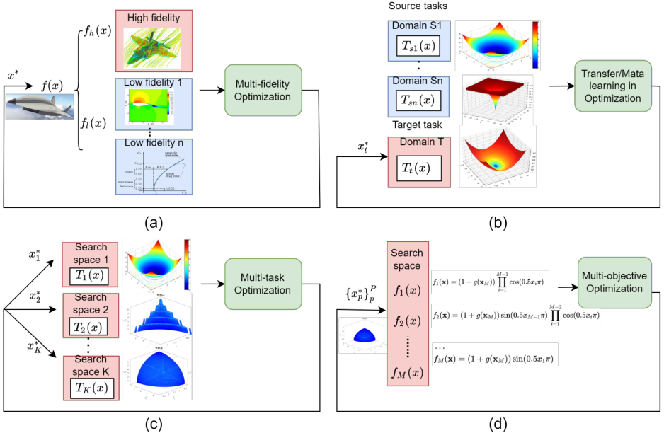
There exist some conceptual similarities and overlaps between multi-task optimization and some other terms, such as multi-objective optimization, multi-fidelity optimization and transfer/meta learning. Similarities and differences are illustrated in Fig. 4. Note that the goal of multi-objective optimization is to handle conflicting objectives of the same task and find optimal tradeoff solutions. By contrast, MTO aims to effectively and concurrently optimize multiple tasks by leveraging the correlated information among different tasks, with each task in MTO being either a single- or multi-objective problem. While multi-fidelity optimization and transfer/meta learning focus on the target task, MTO treats all tasks equal and the knowledge transfer occurs between any related tasks. A detailed description of the differences between these optimization problems can be found in (Zhuang et al. 2020).
Multi-task Bayesian optimization (MTBO) aims to optimize a collection of related tasks at the same time, thereby speeding up the optimization process by taking advantage of the common information across the tasks. There are two requirements to achieve this. First, surrogate models that can learn the transferable knowledge between the tasks should be built. Second, the acquisition function should consider not only the exploration-exploitation balance, but also the correlation between the tasks, so that the data efficiency of optimization can be further improved by transferring knowledge between the related tasks. In the following, we present Bayesian optimization algorithms in which multi-task Gaussian models are constructed and specific acquisition functions are designed for MTO. The need for multi-task learning is ubiquitous across many applications in various fields, such as hyperparameter optimization of machine learning models (Swersky et al. 2013), robotic manipulator inverse dynamics (Dürichen et al. 2014), biomedical engineering, and biomedical engineering (Dürichen et al. 2014). Hence, MLO has drawn considerable attention in the machine learning community, and many MLO models and applications have been explored. Among them, Gaussian process models have been extensively applied to learning a set of tasks on different data sets. More recently, BO has been applied to multi-task learning. In the following, the existing proposed multi-task Bayesian models and Bayesian optimization algorithms for MTL are presented, respectively.
3.6.1. Multi-task Gaussian process
MTO benefits from transferring knowledge across different tasks assuming that the tasks are related to a certain degree. In the geostatistics community, the linear model of coregionalization (LMC) expresses the outputs as linear combinations of independent random functions,
| (24) |
where the latent function is assumed to be a zero-mean Gaussian process with covariance as , and is the coefficient for . In the context of machine learning, many Bayesian multi-task models can be viewed as variations of the LMC with different parameterizations and constraints. A representative work is called multi-task GP (Williams et al. 2007), which uses the intrinsic coregionalization model kernel. Besides the covariance function over inputs , a task covariance matrix is introduced as coregionalization metrics to model the inter-task similarities. Consequently, the product kernel can be derived as follows:
| (25) |
where denotes the Kronecker product, and , is a positive semi-definite matrix, which is guaranteed by the Cholesky decomposition. The multi-task GP suffers from a high computational complexity of . To improve the scalability of MTGP, an efficient learning algorithm using self-measuring similarity is introduced to construct the covariance matrics in (Hayashi et al. 2012).
In LMC models, the correlated process is expressed by a linear combination of a set of independent processes, called instantaneous mixing. Such a method is limited to scenarios where one output process is a blurred version of the other. Alternatively, convolution processes are employed to account for correlations across outputs, and each output can be expressed through a convolution integral between a smoothing kernel and a latent function (Alvarez and Lawrence 2011). However, the approach is criticized for its computational and storage complexity.
For example, Bakker and Heskes (Bakker and Heskes 2003) proposed a Bayesian neural network for MTL in a hierarchical Bayesian perspective. While input-to-hidden weights are shared by all tasks, hidden-to-output weights are task-dependent by placing a prior distribution on the model parameters. Following the similar idea, a more general GP with parametric covariance functions is introduced by Lawrence and Platt (Lawrence and Platt 2004) for MTL and knowledge sharing. Moreover, the informative vector machine is adopted to reduce computation by sparsifying the covariance matrix. Instead of learning the covariance matrix in a parameteric manner, the use of hierarchical Bayesian modeling on GPs is presented by Yu et al. (Yu et al. 2005) and Schwaighofer et al. (Schwaighofer et al. 2005), using a normal-inverse Wishart prior distribution for the mean and covariance function. The assumption behind sharing the same prior over the mean and the covariance matrix is that all tasks are correlated. However, such an assumption may not hold. As a treatment to the outlier tasks, Yu et al. (Yu et al. 2007) presented a robust extension of the previous studies (Yu et al. 2005; Schwaighofer et al. 2005) by using heavier tailed t-Processes. To facilitate efficient inference of the work (Yu et al. 2005), pseudo inputs are adopted to derive a sparse construction for the GP (Lian et al. 2015). As stated in (Zhang and Yang 2021), MTL can boost the performance of reinforcement learning, coined as multi-task reinforcement learning (MRL). Few attempts have been done in this line of research, and some of them has revisited BO. Ghavamzadeh (2010) exploit shared structure in the value functions between related MDPs. However, their approach is designed for on-policy multi-task policy evaluation, rather than computing optimal policies.
3.6.2. Acquisition functions in MTO
Although many attempts have been made to propose multi-task models, only recently a few multi-task Bayesian optimization algorithms have been proposed, especially in the field of hyperparameter optimization in machine learning. Swersky and Snoek (Swersky et al. 2013) extend the multi-task GP (Williams et al. 2007) to Bayesian optimization for knowledge transfer in tuning hyperparameters, where a new AF based on entropy search is proposed by taking cost into consideration. Similar ideas that adopt multi-task GPs or design a new AF introducing a trade-off between information gain and cost minimization can be found in (Moss et al. 2020) and (Klein et al. 2017). Bardenet et al. (Bardenet et al. 2013) considered the hyper-parameter optimization for deep belief networks with different features of the dataset, and proposed collaborative tuning of several problems. While a GP is used to predict the algorithm’s performance, each dataset is visited at each iteration and a new sample is selected by maximizing EI on that dataset.
In contextual policy search (CPS), a joint GP model over the context-parameter space is learned, allowing knowledge acquired from one context to be generalized to similar contexts. ES has been extended to CPS (Metzen 2015) by averaging the expected entropy at different points in a set of randomly sampled contexts. Unfortunately, the performance of sampling-based entropy search is not competitive, and its performance deteriorates in the presence of outliers. Hence, Metzen (Metzen 2016) further investigated minimum regret search to explicitly minimize the expected simple regret. More recently, Thompson sampling has been extended to multi-task optimization by sampling from the posterior to identify the next task and action (Char et al. 2019), which is theoretically guaranteed. Metzen et al. (Metzen et al. 2015) proposed a Bayesian optimization approach (BO-CPS) to handle CPS and adopted the GP-UCB to select parameters for a given context. The global maximizer DIRECT (Jones et al. 1993) is adopted to optimize the GP-UCB.
3.7. Multi-fidelity optimization
Bayesian optimization generally assumes that only the target expensive objective function is available, which is referred to as single-fidelity optimization. In many practical problems, however, the evaluation of the target function can often be run at multiple levels of fidelity with varying costs, , where the higher the fidelity , the more accurate but costly the evaluation will be. For example, in the optimization of the ship hull shape, both low-fidelity inexpensive and high-fidelity expensive hydrodynamic models can be used. This is known as multi-fidelity optimization (MFO), which can be seen as a subclass of multi-task learning, where the group of related functions can be meaningfully ordered by their similarity to the objective function.
MFO aims to accelerate the optimization of the target objective and reduce the optimization cost by jointly learning the maximum amount of information from all fidelity models. To achieve this, Bayesian optimization undertakes two changes to make use of multiple fidelity data, namely multi-fidelity modeling and a new sample selection, which will be discussed in detailed in the following.
3.7.1. Multi-fidelity models
Typically, multi-fidelity Bayesian optimization builds surrogate models of different levels of fidelity either by learning an independent GP for each fidelity (Kandasamy et al. 2016), or jointly modeling multi-fidelity data to capture the correlation between the different fidelity data, such as multi-output GP and deep neural networks. Among them, one most popular multi-fidelity model is Co-Kriging (Myers 1982). Kennedy and O’Hagan (Kennedy and O’Hagan 2000) proposed an autoregressive model to approximate the expensive high-fidelity simulation by the sum of the low-fidelity Kriging model and a discrepancy model , formulated as
| (26) |
where denotes a scaling factor minimizing the discrepancy between and high-fidelity model at the common sampling points. Thus, high-fidelity model can be enhanced by acquiring information from the low-fidelity inexpensive data. Following this basic idea, Forrester et al. (Forrester et al. 2007) and Huang et al. (Huang et al. 2006a) have further investigated the extensions of Co-Kriging to MOPs. Later, a Bayesian hierarchical GP model is developed in (Qian and Wu 2008) to account for complex scale changes from low fidelity to high fidelity. To improve the computational efficiency, a recursive formulation for Co-Kriging was proposed in (Le Gratiet and Garnier 2014), assuming that the training datasets for and have a nested structure, i.e., the training data for the higher fidelity levels is a subset of that of a lower fidelity level. Hence, the GP prior in Eq. 26 is replaced by the corresponding GP posterior, improving the efficiency of the hyperparameter estimations. Following this idea, the autoregressive multi-fidelity model given in Eq. 26 has been generalized by replacing the scaling factor with a non-linear mapping function (Perdikaris et al. 2017).
The multi-fidelity Kriging model has been employed in many domains of research including aerodynamics (Brevault et al. 2020; Bailly and Bailly 2019), engineering design (Keane 2012; Toal et al. 2014), bandit optimisation problems (Song et al. 2019; Sen et al. 2018; Kandasamy et al. 2017), multi-objective optimization problems (Belakaria et al. 2020a) and hyperparameter tuning (Sen et al. 2018). It is worthy of noting that multi-fidelity optimization for bandit problems and MOPs typically focuses on the design of new AFs, which we will present in the following.
3.7.2. Acquisition functions for multi-task optimization
Based on multi-task models (Le Gratiet and Garnier 2014; Kennedy and O’Hagan 2000; Forrester et al. 2007), the design of sophisticated AFs to select both the input locations and the fidelity in the MFO setting has attracted much research interest. Earlier multi-fidelity AFs focused on the adaptation of EI. Huang et al. (Huang et al. 2006a) proposed an augmented EI function to account for different fidelity levels of an infill point. Specifically, the proposed EI is the product of the expectation term, the correlation between the LF and HF models, the ratio of the reduction in the posterior standard deviation after a new replicate is added (Huang et al. 2006b), and the ratio between the evaluation cost of the LF and HF models. To enhance the exploration capability of augmented EI, Liu et al. (Liu et al. 2018) proposed a sample density function that quantifies the distance between the inputs to avoid clustered samples. On the other hand, a new formulation of uncertainty is introduced to the EI in the context of MFO in (Zhang et al. 2018). A recent work develops an adaptive EI to select updating samples, so that a different EI function is used based on which fidelity to query (Hao et al. 2020).A closely related AF to the EI, the KG, also has been applied to the MFP (Wu et al. 2020).
UCB has been widely used in MFO, especially in bandit problems. An early work on principled AF based UCB for MFO is MF-GP-UCB (Kandasamy et al. 2016). The MF-GP-UCB algorithm first formulates an upper bound for each fidelity, among which the minimum bound is identified to be maximized for selecting the new sample. Having selected the new point, a threshold is introduced to decide which fidelity to query. In a follow-up work (Kandasamy et al. 2017), MF-GP-UCB is extended to the continuous fidelity space. Sen et al. (Sen et al. 2018) developed an algorithm based on a hierarchical tree-like partitioning, and employed MF-GP-UCB to select the leaves. The motivation behind this method is to explore coarser partitions at lower fidelities and proceed to finer partitions at higher fidelities when the uncertainty has shrunk. Following this idea, Kandasamy et al. (Kandasamy et al. 2019) adopted MF-GP-UCB to explore the search space at lower fidelities, and then exploit the high fidelities in successively smaller regions. Another plausible way to address bandit problems in multi-fidelity settings is information-based methods. A multi-fidelity mutual-information greedy optimization (MF-MI-Greedy) is introduced in (Song et al. 2019). Each round of MF-MI-Greedy includes an exploration phase to explore the low fidelity actions and an optimization phase to optimize the payoff function at the target fidelity.
Recently, information-theoretic approaches have become popular in MFO. For example, ES with the Co-Kriging model is adopted in (Marco et al. 2017) to solve a two-fidelity optimization. McLeod et al. (McLeod et al. 2017) introduced an environmental variable to denote the varying fidelities, thus a GP can be built on the augmented space. Then, PES is adopted as the AF and a fast sampling strategy is employed to reduce the computational cost. In (Zhang et al. 2017), unknown functions with varying fidelities are jointly modeled as a convolved Gaussian process (Alvarez and Lawrence 2011), then a multi-output random feature approximation is introduced to calculate PES. Since it is non-trivial to calculate the multi-fidelity AFs based on ES/PES, MES has been extended to MFO due to its high computational efficiency (Takeno et al. 2020).
3.8. Transfer/Meta Learning
Although Bayesian optimization offers a powerful data-efficient approach to global black-box optimization problems, it considers each task separately and often starts a search from scratch, which needs a sufficient number of expensive evaluations before achieving high-performance solutions. To combat such a "cold start" issue, transfer/meta learning in Bayesian optimization has attracted a surge of interest in recent years. Given a set of auxiliary/source domains and optimization tasks , a target domain and optimization task , transfer/meta learning in Bayesian optimization aims to leverage knowledge from previous related tasks to speed up the optimization for the target task . A well-studied example is hyperparameter optimization of a machine learning algorithm on a new dataset (target) with observed hyperparameter performances on the other datasets (source/meta-data). The availability of meta-data from previous related tasks in hyperparameter optimization has motivated a simple strategy to speed up the optimization process on a new dataset, called meta-initialization. The core idea behind this is to initialize a hyperparameter search based on the best hyperparameter configurations for similar datasets (Feurer et al. 2015). Typically, the two terms, i.e., transfer/meta learning, are used interchangeably in the context of Bayesian optimization. Note that in the Bayesian optimization community, knowledge transfer has also been investigated under the several umbrellas, including multi-task learning and multi-fidelity optimization, which may overlap with the broad field of transfer learning.
Intuitively, the optimization of target task may suffer from negative transfer if the learned knowledge degrades the performance. Hence, the success of transfer learning is heavily conditioned on the similarity between source and target tasks. According to the method for capturing the similarity, we classify the Bayesian optimization algorithms coupled with transfer learning techniques into the following three groups. The difference between transfer/meta learning and the other notions in the context of BO lies in the problem setup: multi-task learning aims to optimise all tasks simultaneously by allowing knowledge to transfer among them. Multi-fidelity optimization has access to low-fidelity evaluations (source) during the optimization process.
3.8.1. Meta-initialization
The availability of meta-data from previous related tasks in hyperparameter optimization has motivated a simple strategy to speed up the optimization process on a new dataset, called meta-initialization. The core idea behind this is to initial a hyperparameter search based on the best hyperparameter configurations for similar datasets. To achieve this, Feurer et al. (Feurer et al. 2015) introduced a negative Spearman correlation coefficient to measure the similarity between different datasets, while Wistuba et al. (Wistuba et al. 2015) identified the initial hyperparameter configurations via optimising a meta-loss.
3.8.2. Hierarchical model
Hierarchical models learned across the entire datasets arise as a natural solution to making use of the knowledge from related source domains (Tighineanu et al. 2021). For example, Bardenet et al. (Bardenet et al. 2013) noted that the loss values on different datasets may differ in scale, motivating a ranking surrogate to map observations from all runs into the same scale. However, this approach suffers from a high computational complexity incurred by the ranking algorithm. To address this problem, Yogatama and Mann (Yogatama and Mann 2014) suggested to reconstruct the response values by subtracting the per-dataset mean and scaling through the standard deviation, while Golovin et al. (Golovin et al. 2017) proposed an efficient hierarchical GP model using the source posterior mean as the prior mean for the target.
3.8.3. Multi-task Gaussian process
Since multi-task GP models are powerful for capturing the similarity between the source and target tasks, Swersky et al. (Swersky et al. 2013) conducted a straightforward knowledge transfer using a multi-task GP. Meanwhile, the semi-definite (PSD) matrix in multi-task GPs (see Eq. 25) has been modified to improve the computational efficiency (Yogatama and Mann 2014; Min et al. 2020). On the other hand, Joy et al. (Joy et al. 2019) assumed that the source data are noisy observations of the target task, so that the difference between the source and target can be modeled by noise variances. Following this idea, Ramachandran et al. (Ramachandran et al. 2018b) further improved the efficiency of the knowledge transfer by using a multi-bandit algorithm to identify the optimal source.
3.8.4. Weighted combination of GPs
Knowledge transfer in Bayesian optimization can also be achieved by a weighted combination of GPs. Instead of training a single surrogate model on a large training data set (i.e., the historical data), Schilling et al. (Schilling et al. 2016) suggested to use the product of GP experts to improve the learning performance. Specifically, an individual GP is learned on each distinct dataset. This way, the prediction on a target data provided by the product of the individual GPs is a sum of means with weights adjusted with regard to the GP uncertainty. Different strategies have been proposed to adapt the weights in the combination (Da et al. 2019; Feurer et al. 2018). In multi-objective optimization, Min et al. (Min et al. 2017) proposed to identify the weights by optimizing the squared error of out-of-sample predictions. Interestingly, in (Ramachandran et al. 2018a) the location of the global optimum for the target is modeled by combining the distribution of the optimum of each source task. The weight in the mixture distribution is proportional to the similarity between the source and target, which is measured by Kullback-Leibler divergence.
In a complementary direction, a few attempts have been dedicated to leveraging the meta-data within the acquisition function in a similar fashion to the weighted combination of GPs. A representative work is called transfer AF (TAF) (Wistuba et al. 2018), which is defined by the weighted average of the expected improvement on the target dataset and source datasets. More recently, Volpp et al. (Volpp et al. 2020) adopted reinforcement learning to achieve this.
3.9. Parallel/Batch Bayesian optimization
The canonical Bayesian optimization is inherently a sequential process since one new data is sampled in each iteration, which might be inefficient in many applications where multiple data points can be sampled in parallel (Nguyen et al. 2021a). A strength of sequential Bayesian optimization is that a new data point is selected using the maximum available information owing to the immediately updated GP, and therefore searching for multiple query points simultaneously is more challenging. With the growing availability of parallel computing, an increasing number of studies exploring batch Bayesian optimization have been carried out, which can be roughly classified into two groups. One is the extension of the existing AFs to batch selection, and the other is problem reformulation.
3.9.1. Extensions of the existing AFs
A pioneering multi-points acquisition function is the parallelized version of the expected improvement (EI), called q-points EI (q-EI) (Ginsbourger et al. 2008; Ginsbourger et al. 2010). The q-EI is straightforwardly defined as the expected improvement of the points beyond the current best observation. However, the exact calculation of q-EI depends on the integral of q-dimensional Gaussian density, and therefore becomes intractable and intensive as increases. Hence, Ginsbourger et al. (Ginsbourger et al. 2008) sequentially identified points by using Kriging believer or constant liar strategies to replace the unknown output at the last selected point, facilitating the batch selection based on q-EI. Treatments for the intractable calculation of q-EI have been investigated in (Ginsbourger et al. 2010; Wang et al. 2020a; Chevalier and Ginsbourger 2013). Besides, an asynchronous version of q-EI is presented in (Janusevskis et al. 2012).
The parallel extension of the GP-UCB has been widely investigated owing to its theoretical guarantees, i.e., the sublinear growth of cumulative regret. An extension of GP-UCB, called GP-BUCB, is proposed to leverage the updated variance, encouraging more exploration (Desautels et al. 2014). Interestingly, the GP-BUCB has been generalized to a multi-agent distributed setting (Daxberger and Low 2017). Similarly, a GP-UCB approach with pure exploration (GP-UCB-PE) is proposed in (Contal et al. 2013), which identifies the first query point via the GP-UCB, while the remaining ones are selected by maximizing the updated variance. Since MOEAs can provide a set of non-dominated recommendations, they are well-suited for determining the remaining points by simultaneously optimizing the predicted mean and variance (Gupta et al. 2018). In addition, distance exploration can be used to achieve this, avoiding selecting the same query points in a batch (Nguyen et al. 2018). Both GP-BUCB and GP-UCB-PE greedily collect new points by maximizing the information gain estimated by the posterior variance. More diverse batches can be probed by sampling from determinantal point processes (DPPs) (Kathuria et al. 2016; Wang et al. 2017). Similarly, a variant of DPPs, called k-DPPs, is adopted to select a batch of neural network architectures for parallel evaluations (Nguyen et al. 2021a).
With the rapidly growing interest in batch Bayesian optimization, more AFs have been extended to the parallel setting. For example, parallelized PES (Shah and Ghahramani 2015) and KG (q-KG) (Wu and Frazier 2016) are developed to jointly identify a batch of points to probe in the next iteration, rendering, however, a poor scalability to the batch size. Interestingly, a state-of-the-art information-based AF, called trusted-maximizers entropy search (TES), is proposed by introducing trusted maximizers to simplify the information measure (Nguyen et al. 2021b), which is well scalable to the batch size. TS can also be extended to the parallel setting by sampling functions instead (Hernández-Lobato et al. 2016c). More recently, TS has attracted much attention, as the inherent randomness of TS automatically achieves a balance between exploitation and exploration (Kandasamy et al. 2018a). Similarly, it is suggested to sample from a probability distribution over an AF defined by the GP’s hyperparameters (De Palma et al. 2019) , while in (De Ath et al. 2021a), TS is combined with the -greedy acquisition function to account for asynchronous parallel optimization problems (De Ath et al. 2021a). Note that the performance of TS is not necessarily better than traditional AFs, such as EI and UCB.
3.9.2. Problem reformulation
Much effort has been devoted to developing new batch approaches by reformulating the optimization problem of AFs in parallel Bayesian optimization. One interesting direction aims to develop new batch AFs to select input batches that closely match the expected recommendation of sequential methods. For example, a batch objective function minimizing the loss between the sequential selection and the batch is defined in (Azimi et al. 2010), which corresponds to a weighted k-means clustering problem. Given that the sequentially selected inputs are sufficiently different from each other, a maximization-penalization strategy is introduced by adding a local penalty to the AF (González et al. 2016). Liu et al. (Liu et al. 2021) applied a multi-start strategy and gradient-based optimizer to optimize the AF, aiming to identify the local maxima of the AF. In addition, the multi-objective optimizer is a promising approach to finding a batch of query points (Lyu et al. 2018; Zhang et al. 2022), particularly for addressing expensive MOPs (Chugh et al. 2016; Wang et al. 2020b). Similarly, sequentially optimizing multiple AFs is amenable to generating batches of query points (Joy et al. 2020). To better balance exploration and exploitation, different selection metrics can be combined (Gong et al. 2019; Hu et al. 2018). Moreover, in (Wang et al. 2018; Young et al. 2020) local GPs are constructed so that batches of new samples that correspond to each GP can be collected.
4. Challenges and Future Directions
Bayesian optimization is a well-established powerful optimization method for handling expensive black-box problems, which has found many successful real-world applications. Despite all these advances, numerous challenges remain open. In fact, the field of Bayesian optimization keeps very active and dynamic, partly because an increasing number of new applications in science and technology poses new challenges and demands. In the following, we present several most recent important developments in Bayesian optimization and discuss future research directions.
4.1. Distributed Bayesian optimization
Distributed optimization problems are commonly seen in the real world. Despite a proliferation of studies on parallel or batch Bayesian optimization in recent years, most of them require a central server to construct a single surrogate model with few exceptions. For example, a straightforward distributed Bayesian optimization, called HyperSpace, has been proposed by Young et al. (Young et al. 2018; Young et al. 2020) for hyperparameter optimization. HyperSpace partitions the large search space with a degree of overlap and all possible combinations of these hyperspaces are generated and equipped with a GP model, allowing us to run the optimization loop in parallel. Thompson sampling can be fully distributed and handle the asynchronously parallel setting (Hernández-Lobato et al. 2017), although it fails to perform well due to its inherent randomness. Barcos and Cantin (Garcia-Barcos and Martinez-Cantin 2019) presented an interpretation of Bayesian optimization from the Markov decision process perspective and adopted Boltzmann/Gibbs policy to select the next query, which can be performed in a fully distributed manner.
Several questions remain open in design of distributed Bayesian optimization. First, it is of fundamental importance to achieve a trade-off between the convergence rate and communication cost. The convergence of distributed Bayesian optimization needs more rigorous theoretical proof and requires further improvement, and the computational gains will be offset in the presence of communication latencies. Second, it is still barely studied how to handle asynchronous settings that result from time-varying communication costs, different computation capabilities and heterogeneous evaluation times. Third, it is an important yet challenging future direction to take more practical scenarios into consideration, such as complex communication networks and communication constraints.
4.2. Federated Bayesian optimization
While the rapidly growing sensing, storage and computational capability of edge devices has made it possible to train powerful deep models, increasing concern over data privacy has motivated a privacy-preserving decentralized learning paradigm, called federated learning (McMahan et al. 2017). The basic idea in federated learning is that the raw data remains on each client, while models trained on the local data are uploaded to a server to be aggregated, thereby preserving the data privacy. Adapting Bayesian optimization to the federated learning setting is motivated by the presence of black-box expensive machine learning and optimization problems.
Dai et al. (Dai et al. 2020) explored the application of Bayesian optimization in the horizontal federated learning setting, where all agents share the same set of features and their objective functions are defined on a same domain. Federated Thompson sampling (FTS), which samples from the current GP posterior on the server with a probability of and consequently samples from the GP provided by the clients with a probability . However, FTS lacks a rigorous privacy guarantee. To remedy this drawback, differential privacy (Dwork 2008), a mathematically rigorous approach to privacy preservation, is introduced into FTS, called DP-FTS (Dai et al. 2021). More specifically, the DP-FTS partitions the search space into disjoint sub-spaces and then equips each sub-space with an agent. Instead of setting a target agent, DP-FTS adds a central server to perform the DP strategy. After aggregating the model and broadcasting to all agents by the server, the TS is performed on each agent to select the new query.
Instead of using GPs as surrogates, Xu et al. (Xu et al. 2021b) proposed to use radial-basis-function networks (RBFNs) on local clients. A sorting averaging strategy is proposed to construct a global surrogate on the server, where each local RBFN is sorted by a matching metric, and the parameters of each local surrogate are averaged according to the sorted index. To identify new samples, the local and global surrogates work together to provide a mean and variance predictions, and a federated LCB is adopted as an AF. The RBFN-based federated optimization was extended to handle multi/many-objective optimization problems (Xu et al. 2021a).
Although much work addressing challenges in federated learning, including communication efficiency, systems and data heterogeneity, and privacy protection have been reported, privacy-preserving optimization brings with many new questions. First, since GP is non-parameter models, it cannot be directly applied to the federated setting. One idea is to approximate the GP model with random Fourier feature approximates (Dai et al. 2020), in which representative power and computation efficiency should be taken into consideration. Second, Thompson sampling is adopted as AF due to its ability to handle heterogeneous settings; however, it is criticized by its poor performance compared with other AFs. Hence, further investigation in new acquisition method is an interesting yet challenging research direction. Finally, privacy protection in federated Bayesian optimization remains elusive, and more rigorous definitions of threat models in the context of distributed optimization is highly demanded.
4.3. Dynamic optimization
In many real-world applications, such as network resource allocation, recommendation systems, and object tracking, the objective function to be optimized may change over time. Such optimization scenarios are known as dynamic optimization or time-dependent problems. Solving such problems are challenging for most optimization techniques designed for stationary problems (Yazdani et al. 2021). Although various Bayesian optimization algorithms for solving static expensive black-box problems have been proposed, only a few methods have been developed to handle dynamic optimization problems.
Most Bayesian optimization methods for dynamic optimization rely on the multi-armed bandit setting with time-varying reward functions. Bogunovic et al. (Bogunovic et al. 2016) introduced a simple Markov model for the reward functions using GPs, allowing the GP model to vary at a steady rate. Instead of treating all the samples equally important, resetting (Zhao et al. 2020), temporal kernel (Chen and Li 2021), sliding window (Zhou and Shroff 2021), and weighted GP model (Deng et al. 2021) have been proposed to achieve forgetting-remembering trade-off. More recently, a time-dependent objective is optimized at a given future time combined with a two-step look-ahead AF (Renganathan et al. 2021). Nevertheless, the construction of effective surrogates for time-dependent objective functions, the design of acquisition functions to identify promising solutions and track the optimum remain challenging problems. Moreover, it is interesting to incorporate advances in machine learning, such as transfer learning, for leveraging informative from the previous runs.
4.4. Heterogeneous evaluations
Bayesian optimization implicitly assumes that the evaluation cost in different regions of the search space is the same. This assumption, however, can be violated in practice. For example, the evaluation times of different hyperarameter settings and the financial cost for steel or drug design using different ingredients (Abdolshah et al. 2019) may vary dramatically. Moreover, in multi-objective optimization, different objectives may have significantly different computational complexities, known as heterogeneous objective functions (Allmendinger et al. 2015). Handling heterogeneous evaluation costs that arise in both search spaces and objective spaces has attracted increased attention, motivating the development of cost-aware Bayesian optimization.
Most cost-aware Bayesian optimization algorithms focus on single-objective optimization problems. Snoek et al. (Snoek et al. 2012) introduces an AF called expected improvement per second (EIps) to balance between the cost efficiency and evaluation quality via dividing EI by cost. This approach, however, tends to exhibit good performance only when the optimal solution is computationally cheap. To remedy this drawback, a cost-cooling strategy in a cost apportioned Bayesian optimization (CArBO) (Lee et al. 2020) de-emphasizes the heterogeneous costs as the optimization proceeds. Besides, CArBO conducts a cost-effective initialization to achieve a set of cheap and well-distributed initial points, aiming to explore cheaper areas first. In (Lee et al. 2021), an optimization problem constrained by a cost budget is formulated as a constrained Markov decision process and then a rollout AF with a number of look-ahead steps is proposed. The cost-aware Bayesian optimization has also been extended to multi-objective problems where the evaluation costs are non-uniform in the search space (Abdolshah et al. 2019).
To handle heterogeneous computational costs of different objectives in multi-objective optimization, simple Interleaving schemes are developed to fully utilize the available per-objective evaluation budget (Allmendinger et al. 2015). More recently, the search experience of cheap objectives is leveraged to help and accelerate the optimization of expensive ones, thereby enhancing the overall efficiency in solving the problem. For example, Wang et al. (Wang et al. 2021) made use of domain adaptation techniques to align the solutions on/near the Pareto front in a latent space, which allows data augmentation for GPs of the expensive objectives. Alternatively, a co-surrogate model is introduced to capture the relationship between the cheap and expensive objectives in (Wang et al. 2022b). Most recently, a new AF that takes both the search bias and the balance between exploration and exploitation into consideration was proposed (Wang et al. 2022a), thereby reducing the search bias caused by different per-objective evaluation times in multi/many-objective optimization.
Bayesian optimization for heterogeneous settings is still a new research field. This is particularly true when there are many expensive objectives but their computational complexities significantly differ.
4.5. Algorithmic fairness
With the increasingly wider use of machine learning techniques in almost every field of science, technology and human life, there is a growing concern with the fairness of these algorithms. A large body of literature has demonstrated the necessity of avoiding discrimination and bias issues in finance, health care, hiring, and criminal justice that may result from the application of learning and optimization algorithms. A number of unfairness mitigation techniques have been dedicated to measuring and reducing bias/unfairness in different domains, which can be roughly divided into three groups, pre-, in-, and post processing, according to when the technique is applied (Perrone et al. 2021). The first group aims to re-balance the data distribution before training the model. The second group typically trains the model either under fairness constraints or combining accuracy metrics with fairness, while the third group adjust the model after the training process.
Accounting for fairness in the Bayesian optimization framework is a largely unexplored territory with few exceptions. For example, Perrone et al. (Perrone et al. 2021) proposed an in-processing unfairness mitigation method in hyper-parameter optimization based on a constrained Bayesian optimization framework, called FairBO. In FairBO, an additional GP model is trained for the fairness constraint, allowing the constrained EI (cEI) to select new queries that satisfies the constraint. Unfortunately, such a constrained optimization method is designed for a single definition of fairness, which is not always applicable. A different fairness concept was developed in a collaborative Bayesian optimization setting (Sim et al. 2021), in which parties jointly optimize a black-box objective function. It is undesired for each collaborating party to receive unfair rewards while sharing their information with each other. Consequently, a new notion, called fair regret, is introduced based on fairness concepts from economics. Following the notion, the distributed batch GP-UCB is extended using a Gini social-evaluation function to balance the optimization efficiency and fairness.
The fairness problem in the context of Bayesian optimization is vital yet under-studied, and the measurement and mathematical definitions have not been explicit. Hence, the fairness definition should be well-defined at first, so that the fairness requirement can be more precisely integrated into the Bayesian optimization. The second fundamental open question is to investigate how fair surrogate models in Bayesian optimization are and how fair the selected new samples are. Finally, bias reduction strategies in Bayesian optimization can only be applied to the simplest case where a single fairness definition is adopted. The design of practical fairness-aware Bayesian optimization methods is still an open question.
5. Conclusion
Bayesian optimization has become a popular and efficient approach to solving black-box optimization problems, and new methods have been emerging over the last few decades. In this paper, we performed a systematic literature review on Bayesian optimization, focused on new techniques for building the Gaussian process model and designing new acquisition functions to apply Bayesian optimization to various optimization scenarios. We divide these scenarios into nine categories according to the challenges in optimization, including high-dimensional decision and objective spaces, discontinuous search spaces, noise, constraints, and high computational complexity, as well as techniques for improving the efficiency of Bayesian optimization such as multi-task optimization, multi-fidelity optimization, knowledge transfer, and parallelization. Lastly, we summarize most recent developments in Bayesian optimization that address distributed data, data privacy, fairness in optimization, dynamism, and heterogeneity in the objective functions. So far, only sporadic research has been reported in these areas and many open questions remain to be explored.
We hope that this survey paper can help the readers get a clear understanding of research landscape of Bayesian optimization, including its motivation, strengths and limitations, and as well as the future directions that are worth further research efforts.
References
- (1)
- Abdolshah et al. (2019) Majid Abdolshah, Alistair Shilton, Santu Rana, Sunil Gupta, and Svetha Venkatesh. 2019. Cost-aware multi-objective Bayesian optimisation. arXiv preprint arXiv:1909.03600 (2019).
- Agrawal and Goyal (2012) Shipra Agrawal and Navin Goyal. 2012. Analysis of Thompson Sampling for the Multi-armed Bandit Problem. In Proceedings of the 25th Annual Conference on Learning Theory (Proceedings of Machine Learning Research, Vol. 23), Shie Mannor, Nathan Srebro, and Robert C. Williamson (Eds.). PMLR, Edinburgh, Scotland, 39.1–39.26.
- Akbari and Kazerooni (2020) Hossein Akbari and Afshin Kazerooni. 2020. KASRA: A Kriging-based Adaptive Space Reduction Algorithm for global optimization of computationally expensive black-box constrained problems. Applied Soft Computing 90 (2020), 106154.
- Allmendinger et al. (2015) Richard Allmendinger, Julia Handl, and Joshua Knowles. 2015. Multiobjective optimization: When objectives exhibit non-uniform latencies. European Journal of Operational Research 243, 2 (2015), 497–513.
- Alvarez and Lawrence (2011) Mauricio A Alvarez and Neil D Lawrence. 2011. Computationally efficient convolved multiple output Gaussian processes. The Journal of Machine Learning Research 12 (2011), 1459–1500.
- Amri et al. (2021) Reda El Amri, Rodolphe Le Riche, Céline Helbert, Christophette Blanchet-Scalliet, and Sébastien Da Veiga. 2021. A sampling criterion for constrained Bayesian optimization with uncertainties. arXiv preprint arXiv:2103.05706 (2021).
- Antonova et al. (2020) Rika Antonova, Akshara Rai, Tianyu Li, and Danica Kragic. 2020. Bayesian optimization in variational latent spaces with dynamic compression. In Conference on Robot Learning. PMLR, 456–465.
- Ariafar et al. (2019) Setareh Ariafar, Jaume Coll-Font, Dana H Brooks, and Jennifer G Dy. 2019. ADMMBO: Bayesian Optimization with Unknown Constraints using ADMM. J. Mach. Learn. Res. 20, 123 (2019), 1–26.
- Azimi et al. (2010) Javad Azimi, Alan Fern, and Xiaoli Z Fern. 2010. Batch Bayesian optimization via simulation matching. In Advances in Neural Information Processing Systems. Citeseer, 109–117.
- Bailly and Bailly (2019) Joëlle Bailly and Didier Bailly. 2019. Multifidelity aerodynamic optimization of a helicopter rotor blade. AIAA Journal 57, 8 (2019), 3132–3144.
- Bakker and Heskes (2003) BJ Bakker and TM Heskes. 2003. Task clustering and gating for Bayesian multitask learning. Journal of Machine Learning Research (2003), 83–99.
- Baptista and Poloczek (2018) Ricardo Baptista and Matthias Poloczek. 2018. Bayesian optimization of combinatorial structures. In International Conference on Machine Learning. PMLR, 462–471.
- Bardenet et al. (2013) Rémi Bardenet, Mátyás Brendel, Balázs Kégl, and Michele Sebag. 2013. Collaborative hyperparameter tuning. In International conference on Machine Learning. PMLR, 199–207.
- Belakaria and Deshwal (2019) Syrine Belakaria and Aryan Deshwal. 2019. Max-value entropy search for multi-objective Bayesian optimization. In International Conference on Neural Information Processing Systems (NeurIPS).
- Belakaria et al. (2020a) Syrine Belakaria, Aryan Deshwal, and Janardhan Rao Doppa. 2020a. Multi-fidelity multi-objective Bayesian optimization: an output space entropy search approach. In Proceedings of the AAAI Conference on artificial intelligence. 10035–10043.
- Belakaria et al. (2020b) Syrine Belakaria, Aryan Deshwal, Nitthilan Kannappan Jayakodi, and Janardhan Rao Doppa. 2020b. Uncertainty-aware search framework for multi-objective Bayesian optimization. In Proceedings of the AAAI Conference on Artificial Intelligence. 10044–10052.
- Beland and Nair (2017) Justin J Beland and Prasanth B Nair. 2017. Bayesian optimization under uncertainty. In NIPS BayesOpt 2017 workshop.
- Bergstra et al. (2011) James Bergstra, Rémi Bardenet, Yoshua Bengio, and Balázs Kégl. 2011. Algorithms for hyper-parameter optimization. Advances in Neural Information Processing Systems 24 (2011).
- Bergstra et al. (2013) James Bergstra, Dan Yamins, David D Cox, et al. 2013. Hyperopt: A python library for optimizing the hyperparameters of machine learning algorithms. In Proceedings of the 12th Python in Science Conference, Vol. 13. Citeseer, 20.
- Bernardo et al. (2011) J Bernardo, MJ Bayarri, JO Berger, AP Dawid, D Heckerman, AFM Smith, and M West. 2011. Optimization under unknown constraints. Bayesian Statistics 9, 9 (2011), 229.
- Binois et al. (2020) Mickaël Binois, David Ginsbourger, and Olivier Roustant. 2020. On the choice of the low-dimensional domain for global optimization via random embeddings. Journal of Global Optimization 76, 1 (2020), 69–90.
- Binois and Wycoff (2021) Mickael Binois and Nathan Wycoff. 2021. A survey on high-dimensional Gaussian process modeling with application to Bayesian optimization. arXiv preprint arXiv:2111.05040 (2021).
- Bliek et al. (2021) Laurens Bliek, Sicco Verwer, and Mathijs de Weerdt. 2021. Black-box combinatorial optimization using models with integer-valued minima. Annals of Mathematics and Artificial Intelligence 89, 7 (2021), 639–653.
- Bogunovic et al. (2020) Ilija Bogunovic, Andreas Krause, and Jonathan Scarlett. 2020. Corruption-tolerant Gaussian process bandit optimization. In International Conference on Artificial Intelligence and Statistics. PMLR, 1071–1081.
- Bogunovic et al. (2016) Ilija Bogunovic, Jonathan Scarlett, and Volkan Cevher. 2016. Time-varying Gaussian process bandit optimization. In Artificial Intelligence and Statistics. PMLR, 314–323.
- Borovitskiy et al. (2020) Viacheslav Borovitskiy, Alexander Terenin, Peter Mostowsky, and Marc Peter Deisenroth. 2020. Mat’ern Gaussian processes on Riemannian manifolds. arXiv preprint arXiv:2006.10160 (2020).
- Bradford et al. (2018) Eric Bradford, Artur M Schweidtmann, and Alexei Lapkin. 2018. Efficient multiobjective optimization employing Gaussian processes, spectral sampling and a genetic algorithm. Journal of Global Optimization 71, 2 (2018), 407–438.
- Brevault et al. (2020) Loïc Brevault, Mathieu Balesdent, and Ali Hebbal. 2020. Overview of Gaussian process based multi-fidelity techniques with variable relationship between fidelities, application to aerospace systems. Aerospace Science and Technology 107 (2020), 106339.
- Brochu et al. (2010) Eric Brochu, Vlad M Cora, and Nando De Freitas. 2010. A tutorial on Bayesian optimization of expensive cost functions, with application to active user modeling and hierarchical reinforcement learning. arXiv preprint arXiv:1012.2599 (2010).
- Buathong et al. (2020) Poompol Buathong, David Ginsbourger, and Tipaluck Krityakierne. 2020. Kernels over sets of finite sets using RKHS embeddings, with application to Bayesian (combinatorial) optimization. In International Conference on Artificial Intelligence and Statistics. PMLR, 2731–2741.
- Cartis et al. (2021) Coralia Cartis, Estelle Massart, and Adilet Otemissov. 2021. Global optimization using random embeddings. arXiv preprint arXiv:2107.12102 (2021).
- Cartis and Otemissov (2020) Coralia Cartis and Adilet Otemissov. 2020. A dimensionality reduction technique for unconstrained global optimization of functions with low effective dimensionality. arXiv preprint arXiv:2003.09673 (2020).
- Char et al. (2019) Ian Char, Youngseog Chung, Willie Neiswanger, Kirthevasan Kandasamy, Andrew O Nelson, Mark Boyer, Egemen Kolemen, and Jeff Schneider. 2019. Offline contextual Bayesian optimization. Advances in Neural Information Processing Systems 32 (2019), 4627–4638.
- Chen et al. (2012) Bo Chen, Rui Castro, and Andreas Krause. 2012. Joint optimization and variable selection of high-dimensional Gaussian processes. arXiv preprint arXiv:1206.6396 (2012).
- Chen and Tuo (2020) Gecheng Chen and Rui Tuo. 2020. Projection Pursuit Gaussian Process Regression. arXiv preprint arXiv:2004.00667 (2020).
- Chen et al. (2020) Jingfan Chen, Guanghui Zhu, Chunfeng Yuan, and Yihua Huang. 2020. Semi-supervised Embedding Learning for High-dimensional Bayesian Optimization. arXiv preprint arXiv:2005.14601 (2020).
- Chen and Li (2021) Renzhi Chen and Ke Li. 2021. Transfer Bayesian Optimization for Expensive Black-Box Optimization in Dynamic Environment. In 2021 IEEE International Conference on Systems, Man, and Cybernetics (SMC). IEEE, 1374–1379.
- Chen et al. (2021) Wenjie Chen, Shengcai Liu, and Ke Tang. 2021. A New Knowledge Gradient-based Method for Constrained Bayesian Optimization. arXiv preprint arXiv:2101.08743 (2021).
- Cheng et al. (2021) Ji Cheng, Ping Jiang, Qi Zhou, Jiexiang Hu, and Leshi Shu. 2021. A parallel constrained lower confidence bounding approach for computationally expensive constrained optimization problems. Applied Soft Computing 106 (2021), 107276.
- Cheng et al. (2016) Ran Cheng, Yaochu Jin, Markus Olhofer, and Bernhard Sendhoff. 2016. A reference vector guided evolutionary algorithm for many-objective optimization. IEEE Transactions on Evolutionary Computation 20, 5 (2016), 773–791.
- Chevalier et al. (2014) Clément Chevalier, Julien Bect, David Ginsbourger, Emmanuel Vazquez, Victor Picheny, and Yann Richet. 2014. Fast parallel kriging-based stepwise uncertainty reduction with application to the identification of an excursion set. Technometrics 56, 4 (2014), 455–465.
- Chevalier and Ginsbourger (2013) Clément Chevalier and David Ginsbourger. 2013. Fast computation of the multi-points expected improvement with applications in batch selection. In International Conference on Learning and Intelligent Optimization. Springer, 59–69.
- Chugh et al. (2016) Tinkle Chugh, Yaochu Jin, Kaisa Miettinen, Jussi Hakanen, and Karthik Sindhya. 2016. A surrogate-assisted reference vector guided evolutionary algorithm for computationally expensive many-objective optimization. IEEE Transactions on Evolutionary Computation 22, 1 (2016), 129–142.
- Contal et al. (2013) Emile Contal, David Buffoni, Alexandre Robicquet, and Nicolas Vayatis. 2013. Parallel Gaussian process optimization with upper confidence bound and pure exploration. In Joint European Conference on Machine Learning and Knowledge Discovery in Databases. Springer, 225–240.
- Couckuyt et al. (2014) Ivo Couckuyt, Dirk Deschrijver, and Tom Dhaene. 2014. Fast calculation of multiobjective probability of improvement and expected improvement criteria for Pareto optimization. Journal of Global Optimization 60, 3 (2014), 575–594.
- Cressie (1990) Noel Cressie. 1990. The origins of kriging. Mathematical Geology 22, 3 (1990), 239–252.
- Da et al. (2019) Bingshui Da, Yew-Soon Ong, Abhishek Gupta, Liang Feng, and Haitao Liu. 2019. Fast transfer Gaussian process regression with large-scale sources. Knowledge-Based Systems 165 (2019), 208–218.
- Dai et al. (2021) Zhongxiang Dai, Bryan Kian Hsiang Low, and Patrick Jaillet. 2021. Differentially private federated Bayesian optimization with distributed exploration. Advances in Neural Information Processing Systems 34 (2021).
- Dai et al. (2020) Zhongxiang Dai, Kian Hsiang Low, and Patrick Jaillet. 2020. Federated Bayesian optimization via Thompson sampling. arXiv preprint arXiv:2010.10154 (2020).
- Daulton et al. (2021) Samuel Daulton, David Eriksson, Maximilian Balandat, and Eytan Bakshy. 2021. Multi-objective Bayesian optimization over high-dimensional search spaces. arXiv preprint arXiv:2109.10964 (2021).
- Daxberger and Low (2017) Erik A Daxberger and Bryan Kian Hsiang Low. 2017. Distributed batch Gaussian process optimization. In International Conference on Machine Learning. PMLR, 951–960.
- De Ath et al. (2021a) George De Ath, Richard M Everson, and Jonathan E Fieldsend. 2021a. Asynchronous -Greedy Bayesian Optimisation. In Uncertainty in Artificial Intelligence. PMLR, 578–588.
- De Ath et al. (2021b) George De Ath, Richard M Everson, Alma AM Rahat, and Jonathan E Fieldsend. 2021b. Greed is good: Exploration and exploitation trade-offs in Bayesian optimisation. ACM Transactions on Evolutionary Learning and Optimization 1, 1 (2021), 1–22.
- De Palma et al. (2019) Alessandro De Palma, Celestine Mendler-Dünner, Thomas Parnell, Andreea Anghel, and Haralampos Pozidis. 2019. Sampling acquisition functions for batch Bayesian optimization. arXiv preprint arXiv:1903.09434 (2019).
- Delbridge et al. (2020) Ian Delbridge, David Bindel, and Andrew Gordon Wilson. 2020. Randomly projected additive Gaussian processes for regression. In International Conference on Machine Learning. PMLR, 2453–2463.
- Deng et al. (2021) Yuntian Deng, Xingyu Zhou, Baekjin Kim, Ambuj Tewari, Abhishek Gupta, and Ness Shroff. 2021. Weighted Gaussian Process Bandits for Non-stationary Environments. arXiv preprint arXiv:2107.02371 (2021).
- Desautels et al. (2014) Thomas Desautels, Andreas Krause, and Joel W Burdick. 2014. Parallelizing exploration-exploitation tradeoffs in Gaussian process bandit optimization. Journal of Machine Learning Research 15 (2014), 3873–3923.
- Deshwal et al. (2020a) Aryan Deshwal, Syrine Belakaria, and Janardhan Rao Doppa. 2020a. Mercer features for efficient combinatorial Bayesian optimization. arXiv preprint arXiv:2012.07762 (2020).
- Deshwal et al. (2020b) Aryan Deshwal, Syrine Belakaria, and Janardhan Rao Doppa. 2020b. Scalable combinatorial Bayesian optimization with tractable statistical models. arXiv preprint arXiv:2008.08177 (2020).
- Deshwal et al. (2020c) Aryan Deshwal, Syrine Belakaria, Janardhan Rao Doppa, and Alan Fern. 2020c. Optimizing discrete spaces via expensive evaluations: A learning to search framework. In Proceedings of the AAAI Conference on Artificial Intelligence. 3773–3780.
- Deshwal and Doppa (2021) Aryan Deshwal and Jana Doppa. 2021. Combining Latent Space and Structured Kernels for Bayesian Optimization over Combinatorial Spaces. Advances in Neural Information Processing Systems 34 (2021).
- Dürichen et al. (2014) Robert Dürichen, Marco AF Pimentel, Lei Clifton, Achim Schweikard, and David A Clifton. 2014. Multitask Gaussian processes for multivariate physiological time-series analysis. IEEE Transactions on Biomedical Engineering 62, 1 (2014), 314–322.
- Dwork (2008) Cynthia Dwork. 2008. Differential Privacy: A Survey of Results. In TAMC 2008. 1–19.
- Elder (1992) John F Elder. 1992. Global R/sup d/optimization when probes are expensive: the GROPE algorithm. In [Proceedings] 1992 IEEE International Conference on Systems, Man, and Cybernetics. IEEE, 577–582.
- Emmerich et al. (2011) Michael TM Emmerich, André H Deutz, and Jan Willem Klinkenberg. 2011. Hypervolume-based expected improvement: Monotonicity properties and exact computation. In 2011 IEEE Congress of Evolutionary Computation (CEC). IEEE, 2147–2154.
- Emmerich et al. (2006) Michael TM Emmerich, Kyriakos C Giannakoglou, and Boris Naujoks. 2006. Single-and multiobjective evolutionary optimization assisted by Gaussian random field metamodels. IEEE Transactions on Evolutionary Computation 10, 4 (2006), 421–439.
- Eriksson and Jankowiak (2021) David Eriksson and Martin Jankowiak. 2021. High-Dimensional Bayesian Optimization with Sparse Axis-Aligned Subspaces. arXiv preprint arXiv:2103.00349 (2021).
- Eriksson et al. (2019) David Eriksson, Michael Pearce, Jacob Gardner, Ryan D Turner, and Matthias Poloczek. 2019. Scalable global optimization via local Bayesian optimization. Advances in Neural Information Processing Systems 32 (2019), 5496–5507.
- Feurer et al. (2018) Matthias Feurer, Benjamin Letham, and Eytan Bakshy. 2018. Scalable meta-learning for Bayesian optimization. Stat 1050 (2018), 6.
- Feurer et al. (2015) Matthias Feurer, Jost Springenberg, and Frank Hutter. 2015. Initializing Bayesian hyperparameter optimization via meta-learning. In Proceedings of the AAAI Conference on Artificial Intelligence.
- Forrester et al. (2006) Alexander IJ Forrester, Andy J Keane, and Neil W Bressloff. 2006. Design and analysis of "noisy" computer experiments. AIAA journal 44, 10 (2006), 2331–2339.
- Forrester et al. (2007) Alexander IJ Forrester, András Sóbester, and Andy J Keane. 2007. Multi-fidelity optimization via surrogate modelling. Proceedings of the royal society a: mathematical, physical and engineering sciences 463, 2088 (2007), 3251–3269.
- Frazier (2018) Peter I Frazier. 2018. A tutorial on Bayesian optimization. arXiv preprint arXiv:1807.02811 (2018).
- Frazier et al. (2008) Peter I Frazier, Warren B Powell, and Savas Dayanik. 2008. A knowledge-gradient policy for sequential information collection. SIAM Journal on Control and Optimization 47, 5 (2008), 2410–2439.
- Frazier and Wang (2016) Peter I Frazier and Jialei Wang. 2016. Bayesian optimization for materials design. In Information Science for Materials Discovery and Design. Springer, 45–75.
- Fröhlich et al. (2020) Lukas Fröhlich, Edgar Klenske, Julia Vinogradska, Christian Daniel, and Melanie Zeilinger. 2020. Noisy-input entropy search for efficient robust Bayesian optimization. In International Conference on Artificial Intelligence and Statistics. PMLR, 2262–2272.
- Garcia-Barcos and Martinez-Cantin (2019) Javier Garcia-Barcos and Ruben Martinez-Cantin. 2019. Fully distributed Bayesian optimization with stochastic policies. arXiv preprint arXiv:1902.09992 (2019).
- Gardner et al. (2017) Jacob Gardner, Chuan Guo, Kilian Weinberger, Roman Garnett, and Roger Grosse. 2017. Discovering and exploiting additive structure for Bayesian optimization. In Artificial Intelligence and Statistics. PMLR, 1311–1319.
- Gardner et al. (2014) Jacob R Gardner, Matt J Kusner, Zhixiang Eddie Xu, Kilian Q Weinberger, and John P Cunningham. 2014. Bayesian Optimization with Inequality Constraints.. In ICML, Vol. 2014. 937–945.
- Garnett et al. (2010) Roman Garnett, Michael A Osborne, and Stephen J Roberts. 2010. Bayesian optimization for sensor set selection. In Proceedings of the 9th ACM/IEEE International Conference on Information Processing in Sensor Networks. 209–219.
- Garrido-Merchán and Hernández-Lobato (2020) Eduardo C Garrido-Merchán and Daniel Hernández-Lobato. 2020. Dealing with categorical and integer-valued variables in Bayesian optimization with Gaussian processes. Neurocomputing 380 (2020), 20–35.
- Ginsbourger et al. (2008) David Ginsbourger, Rodolphe Le Riche, and Laurent Carraro. 2008. A multi-points criterion for deterministic parallel global optimization based on Gaussian processes. (2008).
- Ginsbourger et al. (2010) David Ginsbourger, Rodolphe Le Riche, and Laurent Carraro. 2010. Kriging is well-suited to parallelize optimization. In Computational Intelligence in Expensive Optimization Problems. Springer, 131–162.
- Goldberg et al. (1997) Paul W Goldberg, Christopher KI Williams, and Christopher M Bishop. 1997. Regression with input-dependent noise: A Gaussian process treatment. Advances in Neural Information Processing Systems 10 (1997), 493–499.
- Golovin et al. (2017) Daniel Golovin, Benjamin Solnik, Subhodeep Moitra, Greg Kochanski, John Karro, and David Sculley. 2017. Google vizier: A service for black-box optimization. In Proceedings of the 23rd ACM SIGKDD International Conference on Knowledge Discovery and Data Mining. 1487–1495.
- Gómez-Bombarelli et al. (2018) Rafael Gómez-Bombarelli, Jennifer N Wei, David Duvenaud, José Miguel Hernández-Lobato, Benjamín Sánchez-Lengeling, Dennis Sheberla, Jorge Aguilera-Iparraguirre, Timothy D Hirzel, Ryan P Adams, and Alán Aspuru-Guzik. 2018. Automatic chemical design using a data-driven continuous representation of molecules. ACS Central Science 4, 2 (2018), 268–276.
- Gong et al. (2019) Chengyue Gong, Jian Peng, and Qiang Liu. 2019. Quantile stein variational gradient descent for batch Bayesian optimization. In International Conference on Machine Learning. PMLR, 2347–2356.
- González et al. (2016) Javier González, Zhenwen Dai, Philipp Hennig, and Neil Lawrence. 2016. Batch Bayesian optimization via local penalization. In Artificial intelligence and statistics. PMLR, 648–657.
- Gonzalvez et al. (2019) Joan Gonzalvez, Edmond Lezmi, Thierry Roncalli, and Jiali Xu. 2019. Financial applications of Gaussian processes and Bayesian optimization. arXiv preprint arXiv:1903.04841 (2019).
- Gramacy et al. (2016) Robert B Gramacy, Genetha A Gray, Sébastien Le Digabel, Herbert KH Lee, Pritam Ranjan, Garth Wells, and Stefan M Wild. 2016. Modeling an augmented Lagrangian for blackbox constrained optimization. Technometrics 58, 1 (2016), 1–11.
- Griffiths and Hernández-Lobato (2020) Ryan-Rhys Griffiths and José Miguel Hernández-Lobato. 2020. Constrained Bayesian optimization for automatic chemical design using variational autoencoders. Chemical Science 11, 2 (2020), 577–586.
- Guo et al. (2019) Dan Guo, Yaochu Jin, Jinliang Ding, and Tianyou Chai. 2019. Heterogeneous ensemble-based infill criterion for evolutionary multiobjective optimization of expensive problems. IEEE Transactions on Cybernetics 49, 3 (2019), 1012–1025.
- Guo et al. (2021) Dan Guo, Xilu Wang, Kailai Gao, Yaochu Jin, Jinliang Ding, and Tianyou Chai. 2021. Evolutionary optimization of high-dimensional multiobjective and many-objective expensive problems assisted by a dropout neural network. IEEE Transactions on Systems, Man, and Cybernetics: systems (2021).
- Gupta et al. (2018) Sunil Gupta, Alistair Shilton, Santu Rana, and Svetha Venkatesh. 2018. Exploiting strategy-space diversity for batch Bayesian optimization. In International Conference on Artificial Intelligence and Statistics. PMLR, 538–547.
- Hao et al. (2020) Peng Hao, Shaojun Feng, Yuwei Li, Bo Wang, and Huihan Chen. 2020. Adaptive infill sampling criterion for multi-fidelity gradient-enhanced kriging model. Structural and Multidisciplinary Optimization 62, 1 (2020), 353–373.
- Hayashi et al. (2012) Kohei Hayashi, Takashi Takenouchi, Ryota Tomioka, and Hisashi Kashima. 2012. Self-measuring similarity for multi-task gaussian process. In Proceedings of ICML Workshop on Unsupervised and Transfer Learning. JMLR Workshop and Conference Proceedings, 145–153.
- Hennig and Schuler (2012) Philipp Hennig and Christian J Schuler. 2012. Entropy Search for Information-Efficient Global Optimization. Journal of Machine Learning Research 13, 6 (2012).
- Hernández-Lobato et al. (2016b) Daniel Hernández-Lobato, Jose Hernandez-Lobato, Amar Shah, and Ryan Adams. 2016b. Predictive entropy search for multi-objective Bayesian optimization. In International Conference on Machine Learning. PMLR, 1492–1501.
- Hernández-Lobato et al. (2015) José Miguel Hernández-Lobato, Michael Gelbart, Matthew Hoffman, Ryan Adams, and Zoubin Ghahramani. 2015. Predictive entropy search for Bayesian optimization with unknown constraints. In International Conference on Machine Learning. PMLR, 1699–1707.
- Hernández-Lobato et al. (2016a) José Miguel Hernández-Lobato, Michael A Gelbart, Ryan P Adams, Matthew W Hoffman, and Zoubin Ghahramani. 2016a. A general framework for constrained Bayesian optimization using information-based search. Journal of Machine Learning Research (2016).
- Hernández-Lobato et al. (2014) José Miguel Hernández-Lobato, Matthew W Hoffman, and Zoubin Ghahramani. 2014. Predictive entropy search for efficient global optimization of black-box functions. arXiv preprint arXiv:1406.2541 (2014).
- Hernández-Lobato et al. (2016c) José Miguel Hernández-Lobato, Edward Pyzer-Knapp, Alan Aspuru-Guzik, and Ryan P Adams. 2016c. Distributed Thompson sampling for large-scale accelerated exploration of chemical space. In NIPS Workshop on Bayesian Optimization.
- Hernández-Lobato et al. (2017) José Miguel Hernández-Lobato, James Requeima, Edward O Pyzer-Knapp, and Alán Aspuru-Guzik. 2017. Parallel and distributed Thompson sampling for large-scale accelerated exploration of chemical space. In International Conference on Machine Learning. PMLR, 1470–1479.
- Hu et al. (2018) Hanbin Hu, Peng Li, and Jianhua Z Huang. 2018. Parallelizable Bayesian optimization for analog and mixed-signal rare failure detection with high coverage. In Proceedings of the International Conference on Computer-Aided Design. 1–8.
- Huang et al. (2006a) Deng Huang, Theodore T Allen, William I Notz, and R Allen Miller. 2006a. Sequential kriging optimization using multiple-fidelity evaluations. Structural and Multidisciplinary Optimization 32, 5 (2006), 369–382.
- Huang et al. (2006b) Deng Huang, Theodore T Allen, William I Notz, and Ning Zeng. 2006b. Global optimization of stochastic black-box systems via sequential kriging meta-models. Journal of Global Optimization 34, 3 (2006), 441–466.
- Hutter et al. (2010) Frank Hutter, Holger H Hoos, and Kevin Leyton-Brown. 2010. Sequential model-based optimization for general algorithm configuration (extended version). Technical Report TR-2010–10, University of British Columbia, Computer Science, Tech. Rep. (2010).
- Hutter et al. (2011) Frank Hutter, Holger H Hoos, and Kevin Leyton-Brown. 2011. Sequential model-based optimization for general algorithm configuration. In International Conference on Learning and Intelligent Optimization. Springer, 507–523.
- Jalali et al. (2017) Hamed Jalali, Inneke Van Nieuwenhuyse, and Victor Picheny. 2017. Comparison of kriging-based algorithms for simulation optimization with heterogeneous noise. European Journal of Operational Research 261, 1 (2017), 279–301.
- Janusevskis et al. (2012) Janis Janusevskis, Rodolphe Le Riche, David Ginsbourger, and Ramunas Girdziusas. 2012. Expected improvements for the asynchronous parallel global optimization of expensive functions: Potentials and challenges. In International Conference on Learning and Intelligent Optimization. Springer, 413–418.
- Jaquier et al. (2021) Noémie Jaquier, Viacheslav Borovitskiy, Andrei Smolensky, Alexander Terenin, Tamim Asfour, and Leonel Rozo. 2021. Geometry-aware Bayesian Optimization in Robotics using Riemannian Mat’ern Kernels. arXiv preprint arXiv:2111.01460 (2021).
- Jaquier and Rozo (2020) Noémie Jaquier and Leonel Rozo. 2020. High-dimensional Bayesian optimization via nested Riemannian manifolds. arXiv preprint arXiv:2010.10904 (2020).
- Jaquier et al. (2019) Noémie Jaquier, Leonel Rozo, Sylvain Calinon, and Mathias Bürger. 2019. Bayesian optimization meets Riemannian manifolds in robot learning. In Conference on Robot Learning. PMLR, 233–246.
- Jeong and Obayashi (2005) Shinkyu Jeong and Shigeru Obayashi. 2005. Efficient global optimization (EGO) for multi-objective problem and data mining. In 2005 IEEE Congress on Evolutionary Computation, Vol. 3. IEEE, 2138–2145.
- Jiao et al. (2019) Ruwang Jiao, Sanyou Zeng, Changhe Li, Yuhong Jiang, and Yaochu Jin. 2019. A complete expected improvement criterion for Gaussian process assisted highly constrained expensive optimization. Information Sciences 471 (2019), 80–96.
- Jones et al. (1993) Donald R Jones, Cary D Perttunen, and Bruce E Stuckman. 1993. Lipschitzian optimization without the Lipschitz constant. Journal of Optimization Theory and Applications 79, 1 (1993), 157–181.
- Jones et al. (1998) Donald R Jones, Matthias Schonlau, and William J Welch. 1998. Efficient global optimization of expensive black-box functions. Journal of Global Optimization 13, 4 (1998), 455–492.
- Joy et al. (2019) Tinu Theckel Joy, Santu Rana, Sunil Gupta, and Svetha Venkatesh. 2019. A flexible transfer learning framework for Bayesian optimization with convergence guarantee. Expert Systems with Applications 115 (2019), 656–672.
- Joy et al. (2020) Tinu Theckel Joy, Santu Rana, Sunil Gupta, and Svetha Venkatesh. 2020. Batch Bayesian optimization using multi-scale search. Knowledge-Based Systems 187 (2020), 104818.
- Kandasamy et al. (2016) Kirthevasan Kandasamy, Gautam Dasarathy, Junier Oliva, Jeff Schneider, and Barnabás Póczos. 2016. Gaussian process optimisation with multi-fidelity evaluations. In Proceedings of the 30th/International Conference on Advances in Neural Information Processing Systems (NIPS’30).
- Kandasamy et al. (2019) Kirthevasan Kandasamy, Gautam Dasarathy, Junier Oliva, Jeff Schneider, and Barnabas Poczos. 2019. Multi-fidelity Gaussian process bandit optimisation. Journal of Artificial Intelligence Research 66 (2019), 151–196.
- Kandasamy et al. (2017) Kirthevasan Kandasamy, Gautam Dasarathy, Jeff Schneider, and Barnabás Póczos. 2017. Multi-fidelity Bayesian optimisation with continuous approximations. In International Conference on Machine Learning. PMLR, 1799–1808.
- Kandasamy et al. (2018a) Kirthevasan Kandasamy, Akshay Krishnamurthy, Jeff Schneider, and Barnabás Póczos. 2018a. Parallelised bayesian optimisation via thompson sampling. In International Conference on Artificial Intelligence and Statistics. PMLR, 133–142.
- Kandasamy et al. (2018b) Kirthevasan Kandasamy, Willie Neiswanger, Jeff Schneider, Barnabas Poczos, and Eric Xing. 2018b. Neural architecture search with Bayesian optimisation and optimal transport. arXiv preprint arXiv:1802.07191 (2018).
- Kandasamy et al. (2015) Kirthevasan Kandasamy, Jeff Schneider, and Barnabás Póczos. 2015. High dimensional Bayesian optimisation and bandits via additive models. In International Conference on Machine Learning. PMLR, 295–304.
- Kathuria et al. (2016) Tarun Kathuria, Amit Deshpande, and Pushmeet Kohli. 2016. Batched Gaussian process bandit optimization via determinantal point processes. Advances in Neural Information Processing Systems 29 (2016), 4206–4214.
- Keane (2006) Andy J Keane. 2006. Statistical improvement criteria for use in multiobjective design optimization. AIAA journal 44, 4 (2006), 879–891.
- Keane (2012) Andy J Keane. 2012. Cokriging for robust design optimization. AIAA journal 50, 11 (2012), 2351–2364.
- Kennedy and O’Hagan (2000) Marc C Kennedy and Anthony O’Hagan. 2000. Predicting the output from a complex computer code when fast approximations are available. Biometrika 87, 1 (2000), 1–13.
- Kersting et al. (2007) Kristian Kersting, Christian Plagemann, Patrick Pfaff, and Wolfram Burgard. 2007. Most likely heteroscedastic Gaussian process regression. In Proceedings of the 24th International Conference on Machine Learning. 393–400.
- Kim et al. (2020) Jungtaek Kim, Minsu Cho, and Seungjin Choi. 2020. Combinatorial Bayesian Optimization with Random Mapping Functions to Convex Polytope. arXiv preprint arXiv:2011.13094 (2020).
- Kirschner et al. (2020) Johannes Kirschner, Ilija Bogunovic, Stefanie Jegelka, and Andreas Krause. 2020. Distributionally robust Bayesian optimization. In International Conference on Artificial Intelligence and Statistics. PMLR, 2174–2184.
- Kirschner and Krause (2019) Johannes Kirschner and Andreas Krause. 2019. Stochastic bandits with context distributions. Advances in Neural Information Processing Systems 32 (2019), 14113–14122.
- Kleijnen (2009) Jack PC Kleijnen. 2009. Kriging metamodeling in simulation: A review. European Journal of Operational Research 192, 3 (2009), 707–716.
- Klein et al. (2017) Aaron Klein, Stefan Falkner, Simon Bartels, Philipp Hennig, and Frank Hutter. 2017. Fast Bayesian optimization of machine learning hyperparameters on large datasets. In Artificial Intelligence and Statistics. PMLR, 528–536.
- Knowles (2006) Joshua Knowles. 2006. ParEGO: A hybrid algorithm with on-line landscape approximation for expensive multiobjective optimization problems. IEEE Transactions on Evolutionary Computation 10, 1 (2006), 50–66.
- Koch et al. (2015) Patrick Koch, Tobias Wagner, Michael TM Emmerich, Thomas Bäck, and Wolfgang Konen. 2015. Efficient multi-criteria optimization on noisy machine learning problems. Applied Soft Computing 29 (2015), 357–370.
- Kodamana et al. (2018) Hariprasad Kodamana, Biao Huang, Rishik Ranjan, Yujia Zhao, Ruomu Tan, and Nima Sammaknejad. 2018. Approaches to robust process identification: A review and tutorial of probabilistic methods. Journal of Process Control 66 (2018), 68–83.
- König et al. (2020) Christopher König, Mohammad Khosravi, Markus Maier, Roy S Smith, Alisa Rupenyan, and John Lygeros. 2020. Safety-aware cascade controller tuning using constrained Bayesian optimization. arXiv preprint arXiv:2010.15211 (2020).
- Kushner (1964) Harold J Kushner. 1964. A new method of locating the maximum point of an arbitrary multipeak curve in the presence of noise. Journal of Basic Engineering 86, 1 (1964), 97–106.
- Kuss (2006a) M. Kuss. 2006a. Gaussian Process Models for Robust Regression, Classification, and Reinforcement Learning. Ph. D. Dissertation. Technische Universität Darmstadt.
- Kuss (2006b) Malte Kuss. 2006b. Gaussian process models for robust regression, classification, and reinforcement learning. Ph. D. Dissertation. Echnische Universität Darmstadt Darmstadt, Germany.
- Kuss et al. (2005) Malte Kuss, Tobias Pfingsten, Lehel Csató, and Carl E Rasmussen. 2005. Approximate inference for robust Gaussian process regression. (2005).
- Lam and Willcox (2017) Remi Lam and Karen Willcox. 2017. Lookahead Bayesian Optimization with Inequality Constraints.. In NIPS. 1890–1900.
- Lam et al. (2016) Remi Lam, Karen Willcox, and David H Wolpert. 2016. Bayesian optimization with a finite budget: An approximate dynamic programming approach. Advances in Neural Information Processing Systems 29 (2016), 883–891.
- Lawrence and Platt (2004) Neil D Lawrence and John C Platt. 2004. Learning to learn with the informative vector machine. In Proceedings of the Twenty-first International Conference on Machine Learning. 65.
- Lázaro-Gredilla and Titsias (2011) Miguel Lázaro-Gredilla and Michalis K Titsias. 2011. Variational heteroscedastic Gaussian process regression. In ICML.
- Le et al. (2005) Quoc V Le, Alex J Smola, and Stéphane Canu. 2005. Heteroscedastic Gaussian process regression. In Proceedings of the 22nd International Conference on Machine Learning. 489–496.
- Le Gratiet and Garnier (2014) Loic Le Gratiet and Josselin Garnier. 2014. Recursive co-kriging model for design of computer experiments with multiple levels of fidelity. International Journal for Uncertainty Quantification 4, 5 (2014).
- Lee et al. (2021) Eric Hans Lee, David Eriksson, Valerio Perrone, and Matthias Seeger. 2021. A Nonmyopic Approach to Cost-Constrained Bayesian Optimization. arXiv preprint arXiv:2106.06079 (2021).
- Lee et al. (2020) Eric Hans Lee, Valerio Perrone, Cedric Archambeau, and Matthias Seeger. 2020. Cost-aware Bayesian optimization. arXiv preprint arXiv:2003.10870 (2020).
- Letham et al. (2020) Benjamin Letham, Roberto Calandra, Akshara Rai, and Eytan Bakshy. 2020. Re-examining linear embeddings for high-dimensional Bayesian optimization. arXiv preprint arXiv:2001.11659 (2020).
- Letham et al. (2019) Benjamin Letham, Brian Karrer, Guilherme Ottoni, and Eytan Bakshy. 2019. Constrained Bayesian optimization with noisy experiments. Bayesian Analysis 14, 2 (2019), 495–519.
- Li et al. (2015) B. Li, J. Li, K. Tang, and X. Yao. 2015. Many-Objective Evolutionary Algorithms: A Survey. AcM Computing Surveys 48, 1 (2015), Article No.: 13, pp 1–35.
- Li et al. (2016) Chun-Liang Li, Kirthevasan Kandasamy, Barnabás Póczos, and Jeff Schneider. 2016. High dimensional Bayesian optimization via restricted projection pursuit models. In Artificial Intelligence and Statistics. PMLR, 884–892.
- Li et al. (2019) Nan Li, Lin Yang, Xiaodong Li, Xiangdong Li, Jiyuan Tu, and Sherman CP Cheung. 2019. Multi-objective optimization for designing of high-speed train cabin ventilation system using particle swarm optimization and multi-fidelity Kriging. Building and Environment 155 (2019), 161–174.
- Li et al. (2018) Zheng Li, Xinyu Wang, Shilun Ruan, Zhaojun Li, Changyu Shen, and Yan Zeng. 2018. A modified hypervolume based expected improvement for multi-objective efficient global optimization method. Structural and Multidisciplinary Optimization 58, 5 (2018), 1961–1979.
- Lian et al. (2015) Wenzhao Lian, Ricardo Henao, Vinayak Rao, Joseph Lucas, and Lawrence Carin. 2015. A multitask point process predictive model. In International Conference on Machine Learning. PMLR, 2030–2038.
- Lin and Roshan Joseph (2020) Li-Hsiang Lin and V Roshan Joseph. 2020. Transformation and additivity in Gaussian processes. Technometrics 62, 4 (2020), 525–535.
- Liu et al. (2020) Haitao Liu, Yew-Soon Ong, Xiaobo Shen, and Jianfei Cai. 2020. When Gaussian process meets big data: A review of scalable GPs. IEEE Transactions on Neural Networks and Learning Systems 31, 11 (2020), 4405–4423.
- Liu et al. (2021) Jingfei Liu, Chao Jiang, and Jing Zheng. 2021. Batch Bayesian optimization via adaptive local search. Applied Intelligence 51, 3 (2021), 1280–1295.
- Liu et al. (2018) Yixin Liu, Shishi Chen, Fenggang Wang, and Fenfen Xiong. 2018. Sequential optimization using multi-level cokriging and extended expected improvement criterion. Structural and Multidisciplinary Optimization 58, 3 (2018), 1155–1173.
- Lorenz et al. (2019) Romy Lorenz, Laura E Simmons, Ricardo P Monti, Joy L Arthur, Severin Limal, Ilkka Laakso, Robert Leech, and Ines R Violante. 2019. Efficiently searching through large tACS parameter spaces using closed-loop Bayesian optimization. Brain Stimulation 12, 6 (2019), 1484–1489.
- Lv et al. (2019) Zhiming Lv, Linqing Wang, Zhongyang Han, Jun Zhao, and Wei Wang. 2019. Surrogate-assisted particle swarm optimization algorithm with Pareto active learning for expensive multi-objective optimization. IEEE/CAA Journal of Automatica Sinica 6, 3 (2019), 838–849.
- Lyu et al. (2018) Wenlong Lyu, Fan Yang, Changhao Yan, Dian Zhou, and Xuan Zeng. 2018. Batch Bayesian optimization via multi-objective acquisition ensemble for automated analog circuit design. In International Conference on Machine Learning. PMLR, 3306–3314.
- Marco et al. (2017) Alonso Marco, Felix Berkenkamp, Philipp Hennig, Angela P Schoellig, Andreas Krause, Stefan Schaal, and Sebastian Trimpe. 2017. Virtual vs. real: Trading off simulations and physical experiments in reinforcement learning with Bayesian optimization. In 2017 IEEE International Conference on Robotics and Automation (ICRA). IEEE, 1557–1563.
- Martinez-Cantin et al. (2017) Ruben Martinez-Cantin, Michael McCourt, and Kevin Tee. 2017. Robust Bayesian optimization with Student-t likelihood. arXiv preprint arXiv:1707.05729 (2017).
- Martinez-Cantin et al. (2018) Ruben Martinez-Cantin, Kevin Tee, and Michael McCourt. 2018. Practical Bayesian optimization in the presence of outliers. In International Conference on Artificial Intelligence and Statistics. PMLR, 1722–1731.
- Marzat et al. (2013) Julien Marzat, Eric Walter, and Hélène Piet-Lahanier. 2013. Worst-case global optimization of black-box functions through Kriging and relaxation. Journal of Global Optimization 55, 4 (2013), 707–727.
- McHutchon and Rasmussen (2011) Andrew McHutchon and Carl Rasmussen. 2011. Gaussian process training with input noise. Advances in Neural Information Processing Systems 24 (2011), 1341–1349.
- McLeod et al. (2017) Mark McLeod, Michael A Osborne, and Stephen J Roberts. 2017. Practical Bayesian optimization for variable cost objectives. arXiv preprint arXiv:1703.04335 (2017).
- McMahan et al. (2017) Brendan McMahan, Eider Moore, Daniel Ramage, Seth Hampson, and Blaise Aguera y Arcas. 2017. Communication-efficient learning of deep networks from decentralized data. In Artificial Intelligence and Statistics. PMLR, 1273–1282.
- Metzen (2015) Jan Hendrik Metzen. 2015. Active contextual entropy search. arXiv preprint arXiv:1511.04211 (2015).
- Metzen (2016) Jan Hendrik Metzen. 2016. Minimum regret search for single-and multi-task optimization. In International Conference on Machine Learning. PMLR, 192–200.
- Metzen et al. (2015) Jan Hendrik Metzen, Alexander Fabisch, and Jonas Hansen. 2015. Bayesian optimization for contextual policy search. In Proceedings of the Second Machine Learning in Planning and Control of Robot Motion Workshop. IROS Hamburg.
- Min et al. (2020) Alan Tan Wei Min, Abhishek Gupta, and Yew-Soon Ong. 2020. Generalizing transfer Bayesian optimization to source-target heterogeneity. IEEE Transactions on Automation Science and Engineering (2020).
- Min et al. (2017) Alan Tan Wei Min, Yew-Soon Ong, Abhishek Gupta, and Chi-Keong Goh. 2017. Multiproblem surrogates: Transfer evolutionary multiobjective optimization of computationally expensive problems. IEEE Transactions on Evolutionary Computation 23, 1 (2017), 15–28.
- Minka (2001) Thomas Peter Minka. 2001. A family of algorithms for approximate Bayesian inference. Ph. D. Dissertation. Massachusetts Institute of Technology.
- Močkus (1975) Jonas Močkus. 1975. On Bayesian methods for seeking the extremum. In Optimization Techniques IFIP Technical Conference. Springer, 400–404.
- Moriconi et al. (2020) Riccardo Moriconi, Marc Peter Deisenroth, and KS Sesh Kumar. 2020. High-dimensional Bayesian optimization using low-dimensional feature spaces. Machine Learning 109, 9 (2020), 1925–1943.
- Moss et al. (2020) Henry B Moss, David S Leslie, and Paul Rayson. 2020. Mumbo: Multi-task max-value Bayesian optimization. arXiv preprint arXiv:2006.12093 (2020).
- Myers (1982) Donald E Myers. 1982. Matrix formulation of co-kriging. Journal of the International Association for Mathematical Geology 14, 3 (1982), 249–257.
- Namura et al. (2017) Nobuo Namura, Koji Shimoyama, and Shigeru Obayashi. 2017. Expected improvement of penalty-based boundary intersection for expensive multiobjective optimization. IEEE Transactions on Evolutionary Computation 21, 6 (2017), 898–913.
- Nayebi et al. (2019) Amin Nayebi, Alexander Munteanu, and Matthias Poloczek. 2019. A framework for Bayesian optimization in embedded subspaces. In International Conference on Machine Learning. PMLR, 4752–4761.
- Nguyen et al. (2020) Dang Nguyen, Sunil Gupta, Santu Rana, Alistair Shilton, and Svetha Venkatesh. 2020. Bayesian optimization for categorical and category-specific continuous inputs. In Proceedings of the AAAI Conference on Artificial Intelligence. 5256–5263.
- Nguyen et al. (2021b) Quoc Phong Nguyen, Zhaoxuan Wu, Bryan Kian Hsiang Low, and Patrick Jaillet. 2021b. Trusted-maximizers entropy search for efficient Bayesian optimization. In Uncertainty in Artificial Intelligence. PMLR, 1486–1495.
- Nguyen et al. (2018) Vu Nguyen, Sunil Gupta, Santu Rana, Cheng Li, and Svetha Venkatesh. 2018. Practical batch Bayesian optimization for less expensive functions. arXiv preprint arXiv:1811.01466 (2018).
- Nguyen et al. (2021a) Vu Nguyen, Tam Le, Makoto Yamada, and Michael A Osborne. 2021a. Optimal transport kernels for sequential and parallel neural architecture search. In International Conference on Machine Learning. PMLR, 8084–8095.
- Nogueira et al. (2016) José Nogueira, Ruben Martinez-Cantin, Alexandre Bernardino, and Lorenzo Jamone. 2016. Unscented Bayesian optimization for safe robot grasping. In 2016 IEEE/RSJ International Conference on Intelligent Robots and Systems (IROS). IEEE, 1967–1972.
- Oh et al. (2018) ChangYong Oh, Efstratios Gavves, and Max Welling. 2018. BOCK: Bayesian optimization with cylindrical kernels. In International Conference on Machine Learning. PMLR, 3868–3877.
- Oh et al. (2019) Changyong Oh, Jakub M Tomczak, Efstratios Gavves, and Max Welling. 2019. Combinatorial Bayesian optimization using the graph cartesian product. arXiv preprint arXiv:1902.00448 (2019).
- O’Hagan (1979) Anthony O’Hagan. 1979. On outlier rejection phenomena in Bayes inference. Journal of the Royal Statistical Society: Series B (Methodological) 41, 3 (1979), 358–367.
- Perdikaris et al. (2017) Paris Perdikaris, Maziar Raissi, Andreas Damianou, Neil D Lawrence, and George Em Karniadakis. 2017. Nonlinear information fusion algorithms for data-efficient multi-fidelity modelling. Proceedings of the Royal Society A: Mathematical, Physical and Engineering Sciences 473, 2198 (2017), 20160751.
- Perrone et al. (2021) Valerio Perrone, Michele Donini, Muhammad Bilal Zafar, Robin Schmucker, Krishnaram Kenthapadi, and Cédric Archambeau. 2021. Fair Bayesian optimization. In Proceedings of the 2021 AAAI/ACM Conference on AI, Ethics, and Society. 854–863.
- Perrone et al. (2019) Valerio Perrone, Iaroslav Shcherbatyi, Rodolphe Jenatton, Cedric Archambeau, and Matthias Seeger. 2019. Constrained Bayesian optimization with max-value entropy search. arXiv preprint arXiv:1910.07003 (2019).
- Perttunen and Stuckman (1990) Cary D Perttunen and Bruce E Stuckman. 1990. The rank transformation applied to a multivariate method of global optimization. IEEE Transactions on Systems, Man, and Cybernetics 20, 5 (1990), 1216–1220.
- Picheny (2014) Victor Picheny. 2014. A stepwise uncertainty reduction approach to constrained global optimization. In Artificial Intelligence and Statistics. PMLR, 787–795.
- Picheny et al. (2013a) Victor Picheny, David Ginsbourger, Yann Richet, and Gregory Caplin. 2013a. Quantile-based optimization of noisy computer experiments with tunable precision. Technometrics 55, 1 (2013), 2–13.
- Picheny et al. (2016) Victor Picheny, Robert B Gramacy, Stefan Wild, and Sébastien Le Digabel. 2016. Bayesian optimization under mixed constraints with a slack-variable augmented Lagrangian. In Proceedings of the 30th International Conference on Neural Information Processing Systems. 1443–1451.
- Picheny et al. (2013b) Victor Picheny, Tobias Wagner, and David Ginsbourger. 2013b. A benchmark of kriging-based infill criteria for noisy optimization. Structural and Multidisciplinary Optimization 48, 3 (2013), 607–626.
- Ponweiser et al. (2008) Wolfgang Ponweiser, Tobias Wagner, Dirk Biermann, and Markus Vincze. 2008. Multiobjective optimization on a limited budget of evaluations using model-assisted -metric selection. In International Conference on Parallel Problem Solving from Nature. Springer, 784–794.
- Qian and Wu (2008) Peter ZG Qian and CF Jeff Wu. 2008. Bayesian hierarchical modeling for integrating low-accuracy and high-accuracy experiments. Technometrics 50, 2 (2008), 192–204.
- Qin et al. (2019) Shufen Qin, Chaoli Sun, Yaochu Jin, and Guochen Zhang. 2019. Bayesian approaches to surrogate-assisted evolutionary multi-objective optimization: a comparative study. In 2019 IEEE Symposium Series on Computational Intelligence (SSCI). IEEE, 2074–2080.
- Quadrianto et al. (2009) Novi Quadrianto, Kristian Kersting, Mark D Reid, Tibério S Caetano, and Wray L Buntine. 2009. Kernel conditional quantile estimation via reduction revisited. In 2009 Ninth IEEE International Conference on Data Mining. IEEE, 938–943.
- Ramachandran et al. (2018a) Anil Ramachandran, Sunil Gupta, Santu Rana, and Svetha Venkatesh. 2018a. Information-theoretic transfer learning framework for Bayesian optimisation. In Joint European Conference on Machine Learning and Knowledge Discovery in Databases. Springer, 827–842.
- Ramachandran et al. (2018b) Anil Ramachandran, Sunil Gupta, Santu Rana, and Svetha Venkatesh. 2018b. Selecting optimal source for transfer learning in Bayesian optimisation. In Pacific Rim International Conference on Artificial Intelligence. Springer, 42–56.
- Ranjit et al. (2019) Mercy Prasanna Ranjit, Gopinath Ganapathy, Kalaivani Sridhar, and Vikram Arumugham. 2019. Efficient deep learning hyperparameter tuning using cloud infrastructure: Intelligent distributed hyperparameter tuning with Bayesian optimization in the cloud. In 2019 IEEE 12th International Conference on Cloud Computing (CLOUD). IEEE, 520–522.
- Rasmussen (2003) Carl Edward Rasmussen. 2003. Gaussian processes in machine learning. In Summer School on Machine Learning. Springer, 63–71.
- Renganathan et al. (2021) S Ashwin Renganathan, Jeffrey Larson, and Stefan M Wild. 2021. Lookahead Acquisition Functions for Finite-Horizon Time-Dependent Bayesian Optimization and Application to Quantum Optimal Control. arXiv preprint arXiv:2105.09824 (2021).
- Rolland et al. (2018) Paul Rolland, Jonathan Scarlett, Ilija Bogunovic, and Volkan Cevher. 2018. High-dimensional Bayesian optimization via additive models with overlapping groups. In International Conference on Artificial Intelligence and Statistics. PMLR, 298–307.
- Ru et al. (2020) Binxin Ru, Ahsan Alvi, Vu Nguyen, Michael A Osborne, and Stephen Roberts. 2020. Bayesian optimisation over multiple continuous and categorical inputs. In International Conference on Machine Learning. PMLR, 8276–8285.
- Ru et al. (2021) Binxin Ru, Xingchen Wan, Xiaowen Dong, and Michael Osborne. 2021. Interpretable Neural Architecture Search via Bayesian Optimisation with Weisfeiler-Lehman Kernels. arXiv preprint arXiv:2006.07556 (2021).
- Russo et al. (2017) Daniel Russo, Benjamin Van Roy, Abbas Kazerouni, Ian Osband, and Zheng Wen. 2017. A tutorial on Thompson sampling. arXiv preprint arXiv:1707.02038 (2017).
- Sacks et al. (1989) Jerome Sacks, William J Welch, Toby J Mitchell, and Henry P Wynn. 1989. Design and analysis of computer experiments. Statist. Sci. 4, 4 (1989), 409–423.
- Sasena (2002) Michael James Sasena. 2002. Flexibility and efficiency enhancements for constrained global design optimization with kriging approximations. University of Michigan.
- Schilling et al. (2016) Nicolas Schilling, Martin Wistuba, and Lars Schmidt-Thieme. 2016. Scalable hyperparameter optimization with products of Gaussian process experts. In Joint European Conference on Machine Learning and Knowledge Discovery in Databases. Springer, 33–48.
- Schonlau et al. (1998) Matthias Schonlau, William J Welch, and Donald R Jones. 1998. Global versus local search in constrained optimization of computer models. Lecture Notes-Monograph Series (1998), 11–25.
- Schwaighofer et al. (2005) Anton Schwaighofer, Volker Tresp, and Kai Yu. 2005. Learning Gaussian process kernels via hierarchical Bayes. In Advances in Neural Information Processing Systems. 1209–1216.
- Scott et al. (2011) Warren Scott, Peter Frazier, and Warren Powell. 2011. The correlated knowledge gradient for simulation optimization of continuous parameters using Gaussian process regression. SIAM Journal on Optimization 21, 3 (2011), 996–1026.
- Sen et al. (2018) Rajat Sen, Kirthevasan Kandasamy, and Sanjay Shakkottai. 2018. Multi-fidelity black-box optimization with hierarchical partitions. In International Conference on Machine Learning. PMLR, 4538–4547.
- Shah and Ghahramani (2015) Amar Shah and Zoubin Ghahramani. 2015. Parallel predictive entropy search for batch global optimization of expensive objective functions. arXiv preprint arXiv:1511.07130 (2015).
- Shahriari et al. (2016) Bobak Shahriari, Kevin Swersky, Ziyu Wang, Ryan P Adams, and Nando De Freitas. 2016. Taking the human out of the loop: A review of Bayesian optimization. Proc. IEEE 104, 1 (2016), 148–175.
- Shimoyama et al. (2012) Koji Shimoyama, Koma Sato, Shinkyu Jeong, and Shigeru Obayashi. 2012. Comparison of the criteria for updating kriging response surface models in multi-objective optimization. In 2012 IEEE Congress on Evolutionary Computation. IEEE, 1–8.
- Siivola et al. (2021) Eero Siivola, Andrei Paleyes, Javier González, and Aki Vehtari. 2021. Good practices for Bayesian optimization of high dimensional structured spaces. Applied AI Letters 2, 2 (2021), e24.
- Sim et al. (2021) Rachael Hwee Ling Sim, Yehong Zhang, Bryan Kian Hsiang Low, and Patrick Jaillet. 2021. Collaborative Bayesian optimization with fair regret. In International Conference on Machine Learning. PMLR, 9691–9701.
- Snoek et al. (2012) Jasper Snoek, Hugo Larochelle, and Ryan P Adams. 2012. Practical Bayesian optimization of machine learning algorithms. Advances in Neural Information Processing Systems 25 (2012).
- Song et al. (2019) Jialin Song, Yuxin Chen, and Yisong Yue. 2019. A general framework for multi-fidelity Bayesian optimization with gaussian processes. In The 22nd International Conference on Artificial Intelligence and Statistics. PMLR, 3158–3167.
- Spagnol et al. (2019) Adrien Spagnol, Rodolphe Le Riche, and Seébastien Da Veiga. 2019. Global sensitivity analysis for optimization with variable selection. SIAM/ASA Journal on Uncertainty Quantification 7, 2 (2019), 417–443.
- Springenberg et al. (2016) Jost Tobias Springenberg, Aaron Klein, Stefan Falkner, and Frank Hutter. 2016. Bayesian optimization with robust Bayesian neural networks. Advances in Neural Information Processing Systems 29 (2016), 4134–4142.
- Srinivas et al. (2009) Niranjan Srinivas, Andreas Krause, Sham M Kakade, and Matthias Seeger. 2009. Gaussian process optimization in the bandit setting: No regret and experimental design. arXiv preprint arXiv:0912.3995 (2009).
- Stuckman (1988) Bruce E Stuckman. 1988. A global search method for optimizing nonlinear systems. IEEE Transactions on Systems, Man, and Cybernetics 18, 6 (1988), 965–977.
- Suzuki et al. (2020) Shinya Suzuki, Shion Takeno, Tomoyuki Tamura, Kazuki Shitara, and Masayuki Karasuyama. 2020. Multi-objective Bayesian optimization using Pareto-frontier entropy. In International Conference on Machine Learning. PMLR, 9279–9288.
- Svenson and Santner (2016) Joshua Svenson and Thomas Santner. 2016. Multiobjective optimization of expensive-to-evaluate deterministic computer simulator models. Computational Statistics & Data Analysis 94 (2016), 250–264.
- Swersky et al. (2020) Kevin Swersky, Yulia Rubanova, David Dohan, and Kevin Murphy. 2020. Amortized Bayesian optimization over discrete spaces. In Conference on Uncertainty in Artificial Intelligence. PMLR, 769–778.
- Swersky et al. (2013) Kevin Swersky, Jasper Snoek, and Ryan Prescott Adams. 2013. Multi-task Bayesian optimization. In Advances in Neural Information Processing Systems. Curran Associates, Inc.
- Takeno et al. (2020) Shion Takeno, Hitoshi Fukuoka, Yuhki Tsukada, Toshiyuki Koyama, Motoki Shiga, Ichiro Takeuchi, and Masayuki Karasuyama. 2020. Multi-fidelity Bayesian optimization with max-value entropy search and its parallelization. In International Conference on Machine Learning. PMLR, 9334–9345.
- Tian et al. (2019) Jie Tian, Ying Tan, Jianchao Zeng, Chaoli Sun, and Yaochu Jin. 2019. Multiobjective infill criterion driven Gaussian process-assisted particle swarm optimization of high-dimensional expensive problems. IEEE Transactions on Evolutionary Computation 23, 3 (2019), 459–472.
- Tighineanu et al. (2021) Petru Tighineanu, Kathrin Skubch, Paul Baireuther, Attila Reiss, Felix Berkenkamp, and Julia Vinogradska. 2021. Transfer Learning with Gaussian Processes for Bayesian Optimization. arXiv preprint arXiv:2111.11223 (2021).
- Toal et al. (2014) David JJ Toal, Andy J Keane, Diego Benito, Jeffery A Dixon, Jingbin Yang, Matthew Price, Trevor Robinson, Alain Remouchamps, and Norbert Kill. 2014. Multifidelity multidisciplinary whole-engine thermomechanical design optimization. Journal of Propulsion and Power 30, 6 (2014), 1654–1666.
- Tran et al. (2020) Anh Tran, Mike Eldred, Scott McCann, and Yan Wang. 2020. srMO-BO-3GP: A sequential regularized multi-objective constrained Bayesian optimization for design applications. In International Design Engineering Technical Conferences and Computers and Information in Engineering Conference, Vol. 83983. American Society of Mechanical Engineers, V009T09A015.
- Turchetta et al. (2020) Matteo Turchetta, Andreas Krause, and Sebastian Trimpe. 2020. Robust model-free reinforcement learning with multi-objective Bayesian optimization. In 2020 IEEE International Conference on Robotics and Automation (ICRA). IEEE, 10702–10708.
- Ungredda and Branke (2021) Juan Ungredda and Juergen Branke. 2021. Bayesian Optimisation for Constrained Problems. arXiv preprint arXiv:2105.13245 (2021).
- ur Rehman et al. (2014) Samee ur Rehman, Matthijs Langelaar, and Fred van Keulen. 2014. Efficient Kriging-based robust optimization of unconstrained problems. Journal of Computational Science 5, 6 (2014), 872–881.
- Van Beers and Kleijnen (2003) Wim CM Van Beers and Jack PC Kleijnen. 2003. Kriging for interpolation in random simulation. Journal of the Operational Research Society 54, 3 (2003), 255–262.
- Vanhatalo et al. (2009) Jarno Vanhatalo, Pasi Jylänki, and Aki Vehtari. 2009. Gaussian process regression with Student-t likelihood. Advances in Neural Information Processing Systems 22 (2009), 1910–1918.
- Vargas-Hernandez (2020) Rodrigo A Vargas-Hernandez. 2020. Bayesian optimization for calibrating and selecting hybrid-density functional models. The Journal of Physical Chemistry A 124, 20 (2020), 4053–4061.
- Vazquez et al. (2008) Emmanuel Vazquez, Julien Villemonteix, Maryan Sidorkiewicz, and Eric Walter. 2008. Global optimization based on noisy evaluations: an empirical study of two statistical approaches. In Journal of Physics: Conference Series. IOP Publishing, 012100.
- Volpp et al. (2020) Michael Volpp, Lukas P Fröhlich, Kirsten Fischer, Andreas Doerr, Stefan Falkner, Frank Hutter, and Christian Daniel. 2020. Meta-learning acquisition functions for transfer learning in Bayesian optimization. arXiv preprint arXiv:1904.02642 (2020).
- Wagner et al. (2010) Tobias Wagner, Michael Emmerich, André Deutz, and Wolfgang Ponweiser. 2010. On expected-improvement criteria for model-based multi-objective optimization. In International Conference on Parallel Problem Solving from Nature. Springer, 718–727.
- Wang et al. (2020c) Haowei Wang, Jun Yuan, and Szu Hui Ng. 2020c. Gaussian process based optimization algorithms with input uncertainty. IISE Transactions 52, 4 (2020), 377–393.
- Wang et al. (2020a) Jialei Wang, Scott C Clark, Eric Liu, and Peter I Frazier. 2020a. Parallel Bayesian global optimization of expensive functions. Operations Research 68, 6 (2020), 1850–1865.
- Wang et al. (2020b) Xilu Wang, Yaochu Jin, Sebastian Schmitt, and Markus Olhofer. 2020b. An adaptive Bayesian approach to surrogate-assisted evolutionary multi-objective optimization. Information Sciences 519 (2020), 317–331.
- Wang et al. (2022a) Xilu Wang, Yaochu Jin, Sebastian Schmitt, and Markus Olhofer. 2022a. Alleviating Search Bias in Bayesian Evolutionary Optimization with Heterogeneous Objectives. (2022). Manuscript submitted for publication.
- Wang et al. (2022b) Xilu Wang, Yaochu Jin, Sebastian Schmitt, and Markus Olhofer. 2022b. Transfer Learning Based Co-surrogate Assisted Evolutionary Bi-objective Optimization for Objectives with Non-uniform Evaluation Times. Evolutionary computation (2022), 1–27.
- Wang et al. (2021) Xilu Wang, Yaochu Jin, Sebastian Schmitt, Markus Olhofer, and Richard Allmendinger. 2021. Transfer learning based surrogate assisted evolutionary bi-objective optimization for objectives with different evaluation times. Knowledge-Based Systems (2021), 107190.
- Wang et al. (2018) Zi Wang, Clement Gehring, Pushmeet Kohli, and Stefanie Jegelka. 2018. Batched large-scale Bayesian optimization in high-dimensional spaces. In International Conference on Artificial Intelligence and Statistics. PMLR, 745–754.
- Wang and Jegelka (2017) Zi Wang and Stefanie Jegelka. 2017. Max-value entropy search for efficient Bayesian optimization. In International Conference on Machine Learning. PMLR, 3627–3635.
- Wang et al. (2017) Zi Wang, Chengtao Li, Stefanie Jegelka, and Pushmeet Kohli. 2017. Batched high-dimensional Bayesian optimization via structural kernel learning. In International Conference on Machine Learning. PMLR, 3656–3664.
- Wang et al. (2013) Ziyu Wang, Masrour Zoghi, Frank Hutter, David Matheson, and Nando De Freitas. 2013. Bayesian optimization in high dimensions via random embeddings. In Twenty-Third International Joint Conference on Artificial Intelligence.
- Williams et al. (2007) Chris Williams, Edwin V Bonilla, and Kian M Chai. 2007. Multi-task Gaussian process prediction. Advances in Neural Information Processing Systems (2007), 153–160.
- Winkel et al. (2021) Munir A Winkel, Jonathan W Stallrich, Curtis B Storlie, and Brian J Reich. 2021. Sequential Optimization in Locally Important Dimensions. Technometrics 63, 2 (2021), 236–248.
- Wistuba et al. (2015) Martin Wistuba, Nicolas Schilling, and Lars Schmidt-Thieme. 2015. Learning hyperparameter optimization initializations. In 2015 IEEE International Conference on Data Science and Advanced Analytics (DSAA). IEEE, 1–10.
- Wistuba et al. (2018) Martin Wistuba, Nicolas Schilling, and Lars Schmidt-Thieme. 2018. Scalable Gaussian process-based transfer surrogates for hyperparameter optimization. Machine Learning 107, 1 (2018), 43–78.
- Wu and Frazier (2016) Jian Wu and Peter Frazier. 2016. The parallel knowledge gradient method for batch Bayesian optimization. Advances in Neural Information Processing Systems 29 (2016), 3126–3134.
- Wu et al. (2020) Jian Wu, Saul Toscano-Palmerin, Peter I Frazier, and Andrew Gordon Wilson. 2020. Practical multi-fidelity Bayesian optimization for hyperparameter tuning. In Uncertainty in Artificial Intelligence. PMLR, 788–798.
- Xu et al. (2020) Hang Xu, Wenhua Zeng, Xiangxiang Zeng, and Gary G Yen. 2020. A polar-metric-based evolutionary algorithm. IEEE Transactions on Cybernetics (2020).
- Xu et al. (2021a) Jinjin Xu, Yaochu Jin, and Wenli Du. 2021a. A federated data-driven evolutionary algorithm for expensive multi-/many-objective optimization. Complex & Intelligent Systems 7, 6 (2021), 3093–3109.
- Xu et al. (2021b) Jinjin Xu, Yaochu Jin, Wenli Du, and Sai Gu. 2021b. A federated data-driven evolutionary algorithm. Knowledge-Based Systems 233 (2021), 107532.
- Yang et al. (2019) Kaifeng Yang, Michael Emmerich, André Deutz, and Thomas Bäck. 2019. Multi-objective Bayesian global optimization using expected hypervolume improvement gradient. Swarm and evolutionary computation 44 (2019), 945–956.
- Yazdani et al. (2021) Danial Yazdani, Ran Cheng, Donya Yazdani, Juergen Branke, Yaochu Jin, , and Xin Yao. 2021. A survey of evolutionary continuous dynamic optimization over two decades – Part A. IEEE Transactions on Evolutionary Computation 25, 4 (2021), 609–629.
- Yogatama and Mann (2014) Dani Yogatama and Gideon Mann. 2014. Efficient transfer learning method for automatic hyperparameter tuning. In Artificial Intelligence and Statistics. PMLR, 1077–1085.
- Young et al. (2018) M Todd Young, Jacob Hinkle, Arvind Ramanathan, and Ramakrishnan Kannan. 2018. Hyperspace: Distributed Bayesian hyperparameter optimization. In 2018 30th International Symposium on Computer Architecture and High Performance Computing (SBAC-PAD). IEEE, 339–347.
- Young et al. (2020) M Todd Young, Jacob D Hinkle, Ramakrishnan Kannan, and Arvind Ramanathan. 2020. Distributed Bayesian optimization of deep reinforcement learning algorithms. J. Parallel and Distrib. Comput. 139 (2020), 43–52.
- Yu et al. (2005) Kai Yu, Volker Tresp, and Anton Schwaighofer. 2005. Learning Gaussian processes from multiple tasks. In Proceedings of the 22nd International Conference on Machine Learning. 1012–1019.
- Yu et al. (2007) Shipeng Yu, Volker Tresp, and Kai Yu. 2007. Robust multi-task learning with -processes. In Proceedings of the 24th International Conference on Machine Learning. 1103–1110.
- Yuan and Wahba (2004) Ming Yuan and Grace Wahba. 2004. Doubly penalized likelihood estimator in heteroscedastic regression. Statistics & Probability Letters 69, 1 (2004), 11–20.
- Yue and Kontar (2020) Xubo Yue and Raed AL Kontar. 2020. Why non-myopic Bayesian optimization is promising and how far should we look-ahead? A study via rollout. In International Conference on Artificial Intelligence and Statistics. PMLR, 2808–2818.
- Zhan et al. (2017) Dawei Zhan, Yuansheng Cheng, and Jun Liu. 2017. Expected improvement matrix-based infill criteria for expensive multiobjective optimization. IEEE Transactions on Evolutionary Computation 21, 6 (2017), 956–975.
- Zhan and Xing (2020) Dawei Zhan and Huanlai Xing. 2020. Expected improvement for expensive optimization: a review. Journal of Global Optimization 78, 3 (2020), 507–544.
- Zhang et al. (2019) Miao Zhang, Huiqi Li, and Steven Su. 2019. High dimensional Bayesian optimization via supervised dimension reduction. arXiv preprint arXiv:1907.08953 (2019).
- Zhang and Li (2007) Qingfu Zhang and Hui Li. 2007. MOEA/D: A multiobjective evolutionary algorithm based on decomposition. IEEE Transactions on evolutionary computation 11, 6 (2007), 712–731.
- Zhang et al. (2009) Qingfu Zhang, Wudong Liu, Edward Tsang, and Botond Virginas. 2009. Expensive multiobjective optimization by MOEA/D with Gaussian process model. IEEE Transactions on Evolutionary Computation 14, 3 (2009), 456–474.
- Zhang et al. (2021a) Shuhan Zhang, Fan Yang, Changhao Yan, Dian Zhou, and Xuan Zeng. 2021a. An Efficient Batch Constrained Bayesian Optimization Approach for Analog Circuit Synthesis via Multi-objective Acquisition Ensemble. IEEE Transactions on Computer-Aided Design of Integrated Circuits and Systems (2021).
- Zhang et al. (2022) Shuhan Zhang, Fan Yang, Changhao Yan, Dian Zhou, and Xuan Zeng. 2022. An Efficient Batch-Constrained Bayesian Optimization Approach for Analog Circuit Synthesis via Multiobjective Acquisition Ensemble. IEEE Trans. Comput. Aided Des. Integr. Circuits Syst. 41, 1 (2022), 1–14.
- Zhang et al. (2020) Yichi Zhang, Daniel W Apley, and Wei Chen. 2020. Bayesian optimization for materials design with mixed quantitative and qualitative variables. Scientific reports 10, 1 (2020), 1–13.
- Zhang et al. (2018) Yu Zhang, Zhong-Hua Han, and Ke-Shi Zhang. 2018. Variable-fidelity expected improvement method for efficient global optimization of expensive functions. Structural and Multidisciplinary Optimization 58, 4 (2018), 1431–1451.
- Zhang et al. (2017) Yehong Zhang, Trong Nghia Hoang, Bryan Kian Hsiang Low, and Mohan Kankanhalli. 2017. Information-based multi-fidelity Bayesian optimization. In NIPS Workshop on Bayesian Optimization.
- Zhang and Yang (2021) Yu Zhang and Qiang Yang. 2021. A survey on multi-task learning. IEEE Transactions on Knowledge and Data Engineering (2021).
- Zhang et al. (2021b) Yunxiang Zhang, Xiangyu Zhang, and Peter Frazier. 2021b. Constrained Two-step Look-Ahead Bayesian Optimization. Advances in Neural Information Processing Systems 34 (2021).
- Zhao et al. (2020) Peng Zhao, Lijun Zhang, Yuan Jiang, and Zhi-Hua Zhou. 2020. A simple approach for non-stationary linear bandits. In International Conference on Artificial Intelligence and Statistics. PMLR, 746–755.
- Zhou et al. (2006) Aimin Zhou, Yaochu Jin, Qingfu Zhang, Bernhard Sendhoff, and Edward Tsang. 2006. Combining model-based and genetics-based offspring generation for multi-objective optimization using a convergence criterion. In 2006 IEEE International Conference on Evolutionary Computation. IEEE, 892–899.
- Zhou et al. (2011) A. Zhou, B. Qu, H. Li, S. Zhao, P. N. Suganthan, and Q. Zhang. 2011. Multiobjective evolutionary algorithms: A survey of the state of the art. Swarm and Evolutionary Computation 1, 1 (2011), 32–49.
- Zhou and Shroff (2021) Xingyu Zhou and Ness Shroff. 2021. No-Regret Algorithms for Time-Varying Bayesian Optimization. In 2021 55th Annual Conference on Information Sciences and Systems (CISS). IEEE, 1–6.
- Zhuang et al. (2020) Fuzhen Zhuang, Zhiyuan Qi, Keyu Duan, Dongbo Xi, Yongchun Zhu, Hengshu Zhu, Hui Xiong, and Qing He. 2020. A comprehensive survey on transfer learning. Proc. IEEE 109, 1 (2020), 43–76.
- Zilinskas et al. (1978) A Zilinskas et al. 1978. Optimization of one-dimensional multimodal functions. Journal of the Royal Statistical Society, Series C (Applied Statistics) 27, 3 (1978).
- Zitzler and Thiele (1999) Eckart Zitzler and Lothar Thiele. 1999. Multiobjective evolutionary algorithms: a comparative case study and the strength Pareto approach. IEEE transactions on Evolutionary Computation 3, 4 (1999), 257–271.
- Zitzler et al. (2003) Eckart Zitzler, Lothar Thiele, Marco Laumanns, Carlos M Fonseca, and Viviane Grunert Da Fonseca. 2003. Performance assessment of multiobjective optimizers: An analysis and review. IEEE Transactions on Evolutionary Computation 7, 2 (2003), 117–132.
- Zmijewski and Meseth (2020) Philipp Zmijewski and Nicolas Meseth. 2020. Evaluation of Bayesian Optimization applied to Discrete-Event Simulation. (2020).