From Attribution Maps to Human-Understandable Explanations through Concept Relevance Propagation
2 Technische Universität Berlin, 10587 Berlin, Germany
3 BIFOLD – Berlin Institute for the Foundations of Learning and Data, 10587 Berlin, Germany
∗ contributed equally
† corresponding authors: {sebastian.lapuschkin,wojciech.samek}@hhi.fraunhofer.de
Abstract
The field of eXplainable Artificial Intelligence (XAI) aims to bring transparency to today’s powerful but opaque deep learning models. While local XAI methods explain individual predictions in form of attribution maps, thereby identifying where important features occur (but not providing information about what they represent), global explanation techniques visualize what concepts a model has generally learned to encode. Both types of methods thus only provide partial insights and leave the burden of interpreting the model’s reasoning to the user. In this work we introduce the Concept Relevance Propagation (CRP) approach, which combines the local and global perspectives and thus allows answering both the “where” and “what” questions for individual predictions. We demonstrate the capability of our method in various settings, showcasing that CRP leads to more human interpretable explanations and provides deep insights into the model’s representation and reasoning through concept atlases, concept composition analyses, and quantitative investigations of concept subspaces and their role in fine-grained decision making.
1 Introduction
Considerable advances have been made in the field of Machine Learning (ML), with especially Deep Neural Networks (DNNs) [72] achieving impressive performances on a multitude of domains [34, 119, 60]. However, the reasoning of these highly complex and non-linear DNNs is generally not obvious [111, 114], and as such, their decisions may be (and often are) biased towards unintended or undesired features [125, 70, 116, 7]. This in turn hampers the transferability of ML models to many application domains of interest, e.g., due to the risks involved in high-stakes decision making [111], or the requirements set in governmental regulatory frameworks [48] and guidelines brought forward [33].
In order to alleviate the “black box” problem and gain insights into the model and its predictions, the field of XAI has recently emerged. In fact, multitudes of XAI methods have been developed that are able to provide explanations of a model’s decision while approaching the subject from different angles, e.g., based on gradients [88, 127], as modified backpropagation processes [13, 124, 120, 91], by probing the model’s reaction to changes in the input [141, 107, 22] or visualizing stimuli specific neurons react strongly to [40, 96]. The field can roughly be divided into local XAI and global XAI . Methods from local XAI commonly compute attribution maps in input space highlighting input regions or features, which carry some form of importance to the individual prediction process (i.e., with respect to a specific sample). However, the visualization of important input regions is often of only limited informative value on its own as it does not tell us what features in particular the model has recognized in those regions, as Figure 1 illustrates.

Furthermore, attribution maps can be understood as a superposition of many different model-internal decision sub-processes (e.g., see [63]), working through various transformations of the same input features and culminating to the final prediction. Many intricacies are lost with local explanation techniques producing only a singular attribution map in the input space per prediction outcome. The result might be unclear, imprecise or even ambiguous explanations.
Assuming for example an image classification setting and an attribution map computed for a specific prediction, it might be clear where (in terms of pixels) important information can be found, but not what this information is, i.e., what characteristics of the raw input features the model has extracted and used during inference, or whether this information is a singular characteristic or an overlapping plurality thereof. This introduces many degrees of freedom to the interpretation of attribution maps generated by local XAI, rendering a precise understanding of the models’ internal reasoning a difficult task.
Global XAI, on the other hand, attempts to address the very issue of understanding the what question, i.e., which features or concepts have been learned by a model or play an important role in a model’s reasoning in general. Some approaches from this category synthesize example data in order to reveal the concept a particular neuron activates for [40, 128, 79, 89, 96], but do not inform which concept is in use in a specific classification or how it can be linked to a specific output. From these approaches, we can at most obtain a global understanding of all possible features the model can use, but how these features interact with each other given some specific data sample and how the model infers a decision remains hidden. Other branches of global XAI propose methods, e.g., to test a model’s sensitivity to a priori known, expected or pre-categorized stimuli [62, 105, 17, 18]. These approaches require labeled data, thus limiting, and standing in contrast to, the exploratory potential of local XAI.
Some recent works have begun to bridge the gap between local and global XAI by, for example, drawing weight-based graphs that show how features interact in a global, yet class-specific scale, but without the capability to deliver explanations for individual data samples [57, 76]. Others plead for creating inherently explainable models in the hope of replacing black box models [111]. These methods, however, either require specialized architectures, data and labels, or training regimes (or a combination thereof) [27, 28] and do not support the still widely used off-the-mill end-to-end trained DNN models with their extended explanation capabilities. A detailed discussion of related work can be found in Supplementary Note A.
In this work, we connect lines of local and global XAI research by introducing Concept Relevance Propagation (CRP) and Relevance Maximization (RelMax), a set of next-generation XAI techniques that explain individual predictions in terms of localized and human-understandable concepts. Other than the related state-of-the-art, CRP and RelMax answer both the “where” and “what” questions of ML model inference, thereby providing deep insights into the model’s reasoning process. As post-hoc XAI methods, CRP and RelMax can be applied to (almost) any ML model with no extra requirements on the data, model or training process. We demonstrate on multiple datasets, model architectures and application domains, that CRP-based analyses allow one to (1) gain insights into the representation and composition of concepts in the model as well as quantitatively investigate their role in prediction, (2) identify and counteract Clever Hans filters [70] focusing on spurious correlations in the data, and (3) analyze whole concept subspaces and their contributions to fine-grained decision making.
Analogously to Activation Maximization [92], our proposed Relevance Maximization approach searches for the most important (in terms of relevance, not activation) examples for latent encodings in, e.g., the training dataset. Together, CRP and RelMax show their advantages in a conducted user study comparing our proposed techniques to various traditional attribution map-based approaches. Finally, where transparency on unique samples are promptly required, the computational efficiency and ease of application of CRP and RelMax quickly provide valuable insights into the model’s representation and decision-making to the human user.
In summary, by lifting XAI to the concept level, CRP and RelMax open up new ways to analyze, debug and interact with ML models, which can be particularly beneficial for safety-critical applications and ML-supported investigations in the sciences.
2 Methods in Brief
This section provides a brief overview over the methodological contributions of this work, i.e. the Concept Relevance Propagation and Relevance Maximization. A more detailed description of our methods can be found in Section 5.
Concept Relevance Propagation in brief. Layer-wise Relevance Propagation (LRP) [13] is a popular method for explaining predictions of a neural network by attributing relevance values to individual input dimensions (e.g., pixels of images). In this process, relevance is propagated backwards through the network, starting from the output until the input layer (see Figure 2a), which also provides relevance values for each intermediate element of the model (e.g., channel of an intermediate layer). Since literature suggests that latent structures of neural networks are encoding abstract human-understandable concepts with distinct semantics, especially in higher layers [142, 96, 104, 18, 24, 47], the channel-wise relevance values can be interpreted as scores quantifying the importance of the corresponding concepts in the inference process.
CRP is an extension of LRP, which disentangles the relevance flows associated with concepts learned by the model via conditional backpropagation. Thus, it allows to compute concept-conditional relevance maps , where represents the data point the model has predicted for and describes a set of conditions (i.e., specifying the explained output category (e.g., “dog”) and concepts as learned and distinctly encoded by model components (e.g., “fur”)), determining the flow of relevance via controlled masking operations in the backward process (see Section 5 for technical details). These concept-conditional explanations show us, e.g., in which part of the image the concepts (encoded in hidden layer channels) “fur” or “eye” are present (the where question) and how much they contribute to the prediction. For the example in Figure 2b it turns out that the concept “fur” is more relevant than the concept “eye” for the prediction “dog”, which is not obvious when looking at explanations from LRP (Figure 2a) or other local attribution methods (e.g. [118, 122, 120, 77]), where the contributions of all concepts are superimposed into a single attribution map.
Please note that condition sets can be chosen by the human stakeholder (i.e., depending on the task), or as we prefer to do in this paper, they can be configured automatically: Per layer we configure algorithmically by ranking the network units in descending order of their relevance values for the current prediction, while choosing layer indices uniformly and arbitrarily from the higher, middle or bottom parts of the models throughout the paper for illustration out of simplicity.

Relevance Maximization in brief. Although CRP allows to compute concept-specific attribution maps by disentangling the backward flow, our understanding of the semantics of latent model structures largely remains elusive with local attributions alone. In other words, the channel-wise relevance values and the concept-conditional relevance maps do not provide the full answer to which specific concept a particular channel is actually encoding (the what question). A canonical approach for gaining insight into the meaning and function of latent model structures is Activation Maximization (ActMax) [142, 96, 104, 24] for generating or selecting samples as representations for concepts encoded in hidden space. We find, however, that (maximizing) the activation of a latent encoding by a given data point does not always correspond to its utility to the model in an inference context (see e.g. [20] or Supplementary Figure 7), putting the faithfulness of activation-based example selection for latent concept representation into question.
We therefore introduce RelMax, as an alternative measure to ActMax, with the objective to maximize the relevance criterion for the selection of representative samples for latent model features (see Section 5 for technical details). For each of the observed concepts, Figure 2c (right) shows 12 image segments from a holdout set, for which channel 274 of layer features.28 of a pre-trained VGG-16 (from [74]) encoding the concept “fur” becomes maximally relevant for the prediction of class “dog”. Since relevance is, other than activation, directly linked to a model’s prediction output, the obtained example sets per latent feature are also highly outcome specific. That is, for a latent feature, we may obtain multiple sets of examples, each illustrating how the model is using a particular feature for the prediction of different outcomes, e.g. classes.
3 Results
Beginning with Section 3.1, we present approaches to study the role of learned concepts in individual predictions using our glocal CRP- and RelMax-based approach. The understanding of hidden features and their function then allows to interact with the model and to test its robustness against feature ablation in Section 3.2. In Section 3.3, we study concept subspaces in order to identify (dis)similarities and roles of concepts in fine-grained decision making. Finally, Section 3.4 examines the benefits of CRP over traditional local XAI methods in a user study.
More detailed investigations can be found in Supplementary Notes D, E and H. In addition, Supplementary Note I provides an example on how CRP can be leveraged to identify systematically learned biases in male vs. female face classification and Supplementary Note J demonstrates the applicability of CRP to time series data.

3.1 Understanding Concept Composition Leading to Prediction
Attribution maps provide only partial insights into the decision making process as they only show where the model is focusing on and not which concepts are actually being used. Figure 3a shows an attribution map computed for the prediction “Northern Flicker”. In this case, the bird’s head — in particular the black eye and red stripe — can be identified as the most relevant part of the image. However, it remains unclear from the explanation whether the color or the shape (or both) of the eye and stripe were the decisive features for the model to arrive at its prediction, and how much these body parts contribute, e.g., compared to the bird’s feathers. Furthermore, as shown in Supplementary Figure 1b attribution maps almost always point to the head or the upper body of a bird, irrespective of the bird explained. Thus, the non-trivial task of interpreting what particular feature of the bird (e.g., color, texture, body part shape or relative position of the body parts) actually led to the decision is put onto the human user, which can result in false conclusions.
By conditioning the explanation on relevant hidden-layer channels via CRP, we can assist in concept understanding and overcome the interpretation gap. Figure 3b shows the result of the CRP analysis. The conditional heatmaps help to localize regions in input space for each relevant concept, and at the same time reveal what the model has picked up in those regions by providing reference samples (i.e., explaining by example). Here, the concepts we identified as “red spot” and “black eyes” (based on our subjective understanding of the representative examples) can be assigned to the head of the Northern Flicker bird. These concepts play a crucial role in the classification of the bird, although, e.g., the “black eyes” concept naturally also occurs in images of cats and dogs. Furthermore, both “dots” concepts affecting the prediction can be assigned to the bird’s torso and the “elongated dots and stripes” concept to the bird’s wings. Note that CRP also allows to quantitatively determine the individual contribution of each concept to the final classification decision by summation of the conditional relevance scores (see Section 5.1). This additional information is very valuable as it indicates, e.g., that the dotted texture is the most relevant feature for this particular prediction, or that color is a very relevant cue (e.g., the masked reference samples for channel 10 are all red and for channel 187 contain only black/brown eyes).
The concept atlas shown in Figure 3c further eases to comprehend the relevant concepts. Technically, the atlas visualizes which concepts are most relevant (and here, second most relevant) in specific input image regions (for details see Supplementary Note B.3.5). By choosing super-pixels as regions of interest, we can aggregate the channel-conditional relevances per super-pixel into regional relevance scores, as discussed in the extended Methods Section in Supplementary Note B.3.2. Here, the concept atlas indicates that the “red spot” and “black eye” concepts are most relevant at the bird’s head, while the two “dots” concepts mostly fill the upper body part. Interestingly, a stripe of red color in the tail feathers of the bird is detected and used by the model, as indicated by the “red spot” concept being second-most relevant in this region. In Supplementary Note E.1 an alternative way for constructing concept atlases using single pixels instead of super-pixels is also discussed.
Alternatively to investigating the most relevant channels overall as in Figure 3b, a region of interest, e.g. a super-pixel, can be chosen and its most relevant concepts studied. A comparison of relevant concepts regarding two regions of unrelated visual features is shown in Supplementary Figures 24, 25 and 26.
With the selection of a specific neuron or concept, Concept Relevance Propagation allows investigating how relevance flows from and through the chosen network unit to lower-level neurons and concepts, as is discussed in Section 5.1. This gives information about which lower-level concepts carry importance for the concept of interest and how it is composed of more elementary conceptual building blocks, which may further improve the understanding of the investigated concept and model as a whole. In Figure 3d, we visualize and analyze the backward flow of relevance scores. The graph-like visualization reveals how concepts in higher layers are composed of lower layer concepts. Here, we show the top-2 concepts influencing our concept of choice, the “animal on branch” concept encoded in features.28 of a VGG-16 model trained on ImageNet. Edges in red color indicate the flow of relevance wrt. to the particular sample from class “Bee Eater” shown to the very right between the visualized filters with corresponding examples and (multi)-conditional heatmaps. The width of each red edge describes the relative strength of contribution of lower layer concepts to their upper layer neighbors. This example shows that different paths in the network potentially activate the filter. Here, concepts that encode feathers, threads or fur together with horizontal structures are responsible for the activation of filter 102 in the observed layer in this particular case. In Supplementary Note J an example on time series data is illustrated.
3.2 Understanding Concept Impact and Reach
In this section, we demonstrate how Concept Relevance Propagation can be leveraged as a Human in the Loop (HITL) solution for dataset analysis. In a first step, we will uncover a Clever Hans artifact [70], suppress it by selectively eliminating the most relevant concepts in order to assess its decisiveness for the recognition of the correct class of a particular data sample. Then, we utilize class-conditional reference sampling (cf. Section 5) to perform an inverse search to identify multiple classes making use of the filter encoding the associated concept, both in a benign and a Clever Hans sense.

In Figure 4a we analyze a sample of the “safe” class of ImageNet in a pretrained VGG-16 BN model. Initially, we obtain an input attribution map highlighting a centered horizontal band of the image, where a watermark is located. If we take a closer look at layer features.30 and perform a local analysis (cf. Section 5) on the watermark, we notice that the five most relevant filters are 203, 361, 483, 454, 414, 486. Visualizing them using ActMax as illustrated in Supplementary Figure 46, we conclude that they approximately encode for white strokes. Using our proposed RelMax approach, which uses CRP for identifying the most relevant samples, we gain a deeper insight into the model’s preferred usage of the filters and discover that the model utilizes them to detect white strokes in “written characters”. A detailed comparison between ActMax and RelMax can be found in Supplementary Note D.1. To test the robustness of the model against this Clever Hans artifact, we successively set the activation output map of the 20 most relevant filters activating on the watermark to zero. In Figure 4a (right), we record the change of classification confidence of four classes with the highest prediction confidence for this sample. From the graph, it can be inferred that the Clever Hans filters focussing on the watermark help the model in prediction, but they are not decisive for correct classification. Thus, the model relies on other potential non-Clever Hans features to detect the safe, verifying the correct functioning of the model in cases of samples without watermarks. Another example with strong dependency on Clever Hans artifacts is found in Supplementary Note H.2.
In an inverse search, we can now explore for which samples and classes these filters also generate high relevance. This allows us to understand the behavior of the filter in more detail and to find other possible contaminated classes. In Figure 4b are the seven most relevant classes for filter 361 illustrated. Surprisingly, many classes including “whistle”, “mop”, “screw”, “mosquito net”, “can opener” and “safe” (among others) in the ImageNet Challenge 2014 data are contaminated with similar watermarks encoded via filter 361 of features.30 which is used for the correct prediction of samples from those classes. To verify our finding, we locate via CRP the source of the filters’ relevance wrt. the true classes in input space and confirm that these filters indeed are used to recognize the characters. This implies that the model has learned a shared Clever Hans artifact spanning over multiple classes to achieve higher accuracy in classification. The high number of contamination of samples with the identified artifactual feature could be explained by the fact that watermarks are sometimes difficult to see with the naked eye (location marked with a black arrow) and thus slip any quality ensuring data inspection. The impact of this image characteristic can, however, be clearly marked using the CRP heatmap. Although the filter is mainly used to detect characters, there are also valid use cases for the model, such as for the puma’s whiskers or the spider’s web. This suggests that the complete removal of Clever Hans concepts through pruning may harm the model in its ability to predict other classes which make valid use of the filter, and that a class-specific correction [7] might be more appropriate.

3.3 Understanding Concept Subspaces, (Dis)Similarities and Roles
So far in our experiments we have treated single filters as functions assumed to (fully) encode learned concept. Consequently, we have visualized examples and quantified effects based on per-filter granularity. While previous work suggest that individual neurons or filters often encode for a single human comprehensible concepts, it can generally be assumed that concepts are encoded by sets of filters (see Supplementary Note A). The learned weights of potentially multiple filters might correlate and thus redundantly encode the same concept, or the directions described by several filters situated in the same layer might span a concept-defining subspace. In this section, we now aim to investigate the encodings of filters of a given neural network layer for similarities in terms of activation and use within the model.
Figure 5a shows an analysis result focusing on a cluster around filter from features.40 of a VGG-16 network with BatchNorm layers trained on ImageNet. The reference samples show various types of typewriter and rectangular laptop keyboard buttons and roofing shingles photographed in oblique perspective, as well as round buttons of typewriters, remote controls for televisions, telephone keys and round turnable dials of various devices and machinery. Thus, the filters around filter 446 seem to cover different aspects of a shared “button” or “small tile” concept. The filters located in this cluster have been identified as similar due to their similar activations over sets of analyzed reference samples (see Section 5.3). Assuming redundancy based on the filter channels’ apparently similar activation behavior, a human could merge them to one encompassing concept, thereby simplifying interpretation by reducing the number of filters in the model. We therefore further investigate the filters 7, 94, 446 and 357 (all showing buttons or keys) in order to find out (1) whether they encode a concept collaboratively, (2) whether they are partly redundant, or (3) whether the cluster serves some discriminative purpose.
Figure 5b visualizes the reference samples of these four filters for the most-relevant classes “laptop computer” and “remote control”. We compute filter activations during a forward pass through the model using instances of both classes as input, as well as filter-conditioned CRP maps for the samples’ respective ground truth class label. Regardless of whether an instance from class “laptop” or “remote control” is chosen as input, the activation maps across the observed channels are in part similar per image, e.g., they all activate on the center diagonal part for the left input image. The per-channel CRP attribution map, however, reveals that while all filters react to similar stimuli in terms of activations, the model seems to use the subtle differences among the observed concepts to distinguish between the classes “laptop” and “remote control”. In both cases, buttons are striking and defining features, and all observed filters activate for button features. However, when computing the conditional heatmaps with CRP for class “remote control”, the activating filters representing round buttons (filters 7 and 94) dominantly receive positive attribution scores, while filter 357 clearly representing typical keyboard button layouts receives negative relevance scores and filter 446 does not receive any relevance despite being reactive to the given input. For samples of class “laptop”, the computation of relevance scores wrt. their true class yields almost opposite attributions, indicating that filters encoding round buttons and dials (filters 94 and 7) provide evidence against class “laptop”, while the activation of channel 357 clearly speaks for the analyzed class as visible in the conditional heatmaps. In both relevance analyses, however, filter 446 receives weak negative to no attributions, presumably as it represents a particular expression of both round and angular buttons which fits (or contradicts) neither of the compared classes particularly well. In fact, filter 446 is highly relevant for class “typewriter keyboard” instead.
In conclusion, we report that although several filters may show signs of correlation in terms of output activation, they are not necessarily encoding redundant information or are serving the same purpose. Conversely, using our proposed Concept Relevance Propagation in combination with the Relevance Maximization-based process for selecting reference examples representing seemingly correlating filters, we are able to discover and understand the subtleties a neural network has learned to encode in its latent representations. See Supplementary Note H.4 for additional results in extension to this section.
3.4 Human Evaluation Study
This section presents the results of a human evaluation study, which we performed to assess the practical utility of the CRP- and RelMax-based explanations to (non-expert) end users for understanding ML model behavior. Human subjects were asked to decide — based on explanations — whether the model’s prediction has been influenced by the presence of a particular and known data artifact or not. We trained two image classifiers, of which one has learned to utilize a data artifact — a thick black border around the image (see Figure 6a). For both models, we then generate explanations (see Figure 6b and Figure 6c) on images containing the artifact, using the proposed CRP maps with RelMax examples as well as four popular XAI methods, namely Integrated Gradients (IG) [127], SHAP [77], Grad-CAM [118] and LRP [13]. In the primary task, the participants are asked to assess, whether the black border impacts the model prediction according to the explanation (binary answer: yes or no). Furthermore, we ask secondary questions on how confident they are in their answer and about the perceived clarity of the presented explanations. For more details on the study setup, we refer the reader to Section 5.4.

The results of the study consistently show that participants were reliably able to detect whether the prediction was impacted by the border artifact when exposed to CRP- and RelMax explanations (see Figure 6d). CRP shows the highest true positive (TPR) and true negative (TNR) rates of and , respectively, and thus results in an accuracy (wrt. the primary task) which is significantly higher than that of all other methods (two-sample -test -values of less than ), as shown in the Supplementary Table 3. The study participants obtained the second best results when exposed to Grad-CAM explanations with a TPR and TNR of and , respectively. Participants exposed to explanations from IG performed worst with and , respectively. It is to note, that random guessing would correspond to values of 50 %, indicating that the insight obtainable from IG explanations is limited in this study. We note that in general it seems to be easier to detect a model’s use of the introduced border artifact through all evaluated XAI approaches, than it is to correctly reject an impact of the artifact, since for all methods we observe TPR TNR.
When inspecting the proclaimed confidence with which the participants made their prediction, a direct link does not seem to exist to the measured prediction performance when assessing the artifact’s impact. Interestingly, participants exposed to the IG explanations report the highest confidence (approx. 77 %) — while at the same time performing worst in the primary task — followed by CRP (approx. 76 % self-rated confidence). These results support the findings of [62], that traditional (i.e. single per sample and class, as shown in Figure 6b) saliency- or attribution maps alone might be misleading and insufficient for understanding the reasoning of a machine learning predictor, e.g., see the IG heatmap. Regarding clarity of the explanations as perceived by the participants, the fine-grained attribution maps of IG and LRP receive the highest scores. CRP and RelMax interestingly result in the lowest reported clarity, which might be linked to the more complex nature of the method, potentially leaving some of the participants overwhelmed with the increased amount of information to process, and time required to do so. This result is consistent with the observation of Hacker and Passoth [51] that addressees prefer simple and concise explanations. Despite that, our results demonstrate that our proposed approach is the most effective option for the participants to solve the primary task of the study.
4 Discussion
In this work we have introduced Concept Relevance Propagation, a post-hoc explanation method, which not only indicates which part of the input is relevant for an individual prediction, but also communicates the meaning of involved latent representations by providing human-understandable examples. Since CRP combines the benefits of the local and global XAI perspective, it computes more detailed and contextualized explanations, considerably extending the state-of-the-art. Among its advantages are the high computational efficiency (within the order of a backward pass to compute near-instantaneous local explanations for the most relevant concepts, and a complete concept atlas visualization within the order of seconds) and the out-of-the-box applicability to (almost) any model without imposing constraints on the training process, the data and label availability, or the model architecture. Furthermore, CRP introduces the idea of conditional backpropagation tied to a single concept or a combination of concepts as encoded by the model, within or across layers. Via this ansatz, the contribution of all neurons’ concepts in a layer can be faithfully attributed, localized in the input space, and finally their interaction can be studied. As shown in this work, such an analysis allows one to disentangle and separately explain the multitude of in-parallel partial forward processes, which transform and combine features and concepts before culminating into a prediction. Finally, with Relevance Maximization we move beyond the decade-old practice of communicating latent features of neural networks based on examples obtained via maximized activation. In particular, we show that the examples which stimulate hidden features maximally are not necessarily useful for the model in an inference context, or representative for the data the model is familiar and confident with. By providing examples based on relevance, however, the user is presented with data with characteristics which actually play an important role in the prediction process. Since the user can select examples wrt. any (i.e., not necessarily the ground truth) output class, our approach constitutes a new tool to systematically investigate latent concepts in neural networks.
Our experiments have qualitatively and quantitatively demonstrated the additional value of the CRP approach for common datasets and end-to-end trained models. Specifically, we showed that reference samples selected with relevance-based criteria, concept heatmaps and atlases, as well as concept composition graphs open up the ability to understand model reasoning on a more abstract and conceptual level. These insights then allowed us to identify Clever Hans concepts, to investigate their impact, and finally to correct for these misbehaviors. Further, using our relevance-based reference sample sets, we were able to identify concept themes spanned by sets of filters in latent space. Although channels of a cluster have a similar function, they seem to be used by the model for fine-grained decisions regarding details in the data, such as the particular type of buttons to partially decide whether an image shows a laptop keyboard, a mechanical typewriter or a TV remote control. In addition, we have demonstrated the usefulness of CRP in non-image data domain, where traditional attribution maps are often difficult to interpret and comprehend by the user. Our experiments on time series data have shown that as long as a visualization of the data can be found, the meaning of latent concepts can be communicated via reference examples. Finally, we did conduct a user study which validates a significant increase in utility of our glocal CRP- and RelMax-based approach above traditional post-hoc local XAI methods for understanding a model’s inference behavior by human assessors. For completeness, we would like to make the reader aware of two factors possibly affecting the outcome of our study, namely the potentially varying degree of technical and in-domain training of the study participants, as well as the given prior knowledge about the nature of the data artifact potentially affecting the model. Both factors should therefore be addressed and evaluated individually in future work, e.g., in order to assess the potential of (g)local XAI approaches for assessing yet unexplored model behavior based on feedback for single instance predictions, across different levels of expert knowledge.
Overall, we believe that the tools we have proposed in this work, and the resulting increase in semantics and detail to be found in sample-specific neural network explanations, will advance the applicability of post-hoc eXplainable Artificial Intelligence to novel or previously difficult to handle models, problems and data domains.
5 Methods
This section presents the techniques used and introduced in this paper in brief. For an elaborate introduction and discussion, please refer to Supplementary Notes B and C. For an estimation of run time requirements, the computational steps involved, as well as for guidelines on the interpretation of the output obtained by our techniques, please refer to Supplementary Note F.
5.1 Concept Relevance Propagation
In the following, we introduce CRP, a backpropagation-based attribution method extending the framework of LRP [13].
As such, Concept Relevance Propagation inherits the basic assumptions and properties of LRP.
LRP Revisited. Assuming a predictor with layers
| (1) |
LRP follows the flow of activations computed during the forward pass through the model in opposite direction, from the final layer back to the input mapping . Given a particular mapping , we consider its pre-activations mapping inputs to outputs and their aggregations at . Commonly in neural network architectures such a computation is given with
| (2) | ||||
| (3) | ||||
| (4) |
where are the layer’s inputs and its weight parameters. Finally, constitutes a (component-wise) non-linearity producing input activation for the succeeding layer(s). The LRP method distributes relevance quantities corresponding to and received from upper layers towards lower layers proportionally to the relative contributions of to , i.e.,
| (5) |
Lower neuron relevance is obtained by losslessly aggregating all incoming relevance messages as
| (6) |
This process ensures the property of relevance conservation between a neuron and its inputs , and thus adjacent layers. LRP is mathematically founded in Deep Taylor Decomposition [85].
Disentangling Explanations with CRP. Concept Relevance Propagation extends the formalism of LRP by introducing conditional relevance propagation determined by a set of conditions . Each condition can be understood as an identifier for neural network elements, such as neurons located in some layer, representing latent encodings of concepts of interest. One such condition could, for example, represent a particular network output to initiate the backpropagation process from. Within the CRP framework, the basic relevance decomposition formula of LRP given in Equation (5) then becomes
| (7) |
following the potential for a “filtering” functionality briefly discussed in [86]. Here, is the relevance assigned to layer output given from the CRP process performed in upper layers under conditions , to be distributed to lower layers. The sum-loop over then “selects” via the Kronecker-Delta neurons of which the relevance is to be propagated further, given corresponds to concepts as specified in set specific to layer . The result is the concept-conditional relevance message carrying the relevance quantities wrt. the prediction outcome on conditioned to and . Note that the sum is not particularly necessary in Equation (7), but serves as a means to compare all possible for identity to the current . In practice , CRP can be implemented efficiently as a single backpropagation step by binary masking of relevance tensors, and is compatible to the recommended rule composites for relevance backpropagation [84, 65]. We provide an efficient implementation of CRP based on Zennit [6] at https://github.com/rachtibat/zennit-crp.
The effect of CRP over LRP and other attribution methods is an increase in detail of the obtained explanations. Given a typical image classification Convolutional Neural Network (CNN), one may assume the computation of three-dimensional latent tensors, where the first two axes span the application coordinates of spatially invariant convolutional filters, which generate output activations stored in the channels of the third axis. For simplicity, one can further assume that each filter channel is associated to exactly one latent concept. Neurons can thus be grouped into spatial and channel axes in order to restrict the application of CRP conditions to the channel axis only, i.e.,
| (8) |
Here, the tuple uniquely addresses an output voxel of the activation tensor computed during the forward pass with and indicating the spatial tensor positions and the channel. Figure 2a exemplarily contrasts the attribution-based explanation wrt. class “dog” only (which also is possible with LRP and other attribution methods) as , to the attributions for, e.g., “dog fur” as (possible with CRP only) by conditionally masking channels responsible for fur pattern representations. Alternatively, conditions can be notated in the form of , to provide a more explicit notation specifying the affiliation of concepts to distinct layers. Here we use the terms fur and dog describing latent or labelled concepts, respectively, as proxy representations for network element identifiers . We further assume that in any layer without explicit designation of conditions all -operators always evaluate to to not restrict the flow of attributions through these layers.
Due to the conservation property of CRP inherited from LRP, the global relevance of individual concepts to per-sample inference can be measured by summation over input units as
| (9) |
in any layer where has taken full effect. This can easily be extended to a localized analysis of conceptual importance, by restricting the relevance aggregations to regions of interest
| (10) |
as also illustrated in Supplementary Figure 3. Additionally, as shown in Supplementary Figure 4, an aggregation of the relevance messages may be utilized to identify dependencies of a concept encoded by channels , to concepts encoded by channels in a lower layer, in context of the prediction of a sample and CRP-conditions . With an expansion of the indexing of downstream target voxels wrt. Equation (9) as
| (11) |
the tuple addresses the spatial axes with and , and the channel axis at layer . An aggregation over spatial axes with
| (12) |
communicates the dependency between channel to lower-layer channel , and thus related concepts, in terms of relevance in the prediction context of sample . Following the LRP methodology, an adaptation of the CRP approach beyond CNN, e.g., to recurrent [10] or graph [115] neural networks, is possible. Further details on our proposed Concept Relevance Propagation method are given in Supplementary Note B.
5.2 Selecting Reference Examples
In the following, we discuss the widely-used Activation Maximization approach to procuring representations for latent neurons, and present our novel CRP-based Relevance Maximization technique to improve concept identification and understanding. An in-depth introduction to all details of our proposed technique is given in Supplementary Note C, with various modes of application and analyses being discussed in Supplementary Note D.
5.2.1 Activation Maximization
A large part of feature visualization techniques rely on ActMax, where in its simplest form, input images are sought that give rise to the highest activation value of a specific network unit. Recent work [137, 28] proposes to select reference samples from existing data for feature visualization and analysis. In the literature, the selection of reference samples for a chosen concept manifested in groups of neurons is often based on the strength of activation induced by a sample. For data-based reference sample selection, the possible input space is restricted to elements of a particular finite dataset . The authors of [28] assume convolutional layer filters to be spatially invariant. Therefore, entire filter channels instead of single neurons are investigated for convolutional layers. One particular choice of maximization target is to identify samples , which maximize the sum over all channel activations, i.e.,
| (13) |
resulting in samples which are likely to show a channel’s concept in multiple (spatially distributed) input features, as maximizing the entire channel also maximizes . However, while targeting all channel neurons, reference samples including both concept-supporting and contradicting features might result in a low function output of , as negative activations are taken into account by the sum. Alternatively, a non-linearity can be applied on , e.g., ReLU, to only consider positive activations. A different choice is to define maximally activating samples by observing the maximum channel activation
| (14) |
leading to samples with a more localized and strongly activating set of input features characterizing a channel’s concept. These samples might be more difficult to interpret, as only a small region of a sample might express the concept.
In order to collect multiple reference images describing a concept, the dataset consisting of samples is first sorted in descending order according to the maximization target , i.e.
| (15) |
Subsequently, we define the set
| (16) |
containing the samples ranked first according to the maximization target to represent the concept of the filter(s) under investigation. We denote the set of samples obtained from as and the set obtained from as .
5.2.2 Relevance Maximization
We introduce the method of RelMax as a complement to Activation Maximization. Regarding RelMax, we do not search for images that produce a maximal activation response. Instead, we aim to find samples, which contain the relevant concepts for a prediction. In order to select the most relevant samples, we define maximization targets by using the relevance of neuron for a given prediction, instead of its activation value . Specifically, the maximization targets are given as
| (17) |
By utilizing relevance scores instead of relying on activations only, the maximization target or is class- (true, predicted or arbitrarily chosen, depending on ), model-, and potentially concept-specific (depending on ), as is also illustrated in Supplementary figure 7a. The resulting set of reference samples thus includes only samples which depict facets of a concept that are actually useful for the model during inference (see figure 7b). How differences in resulting reference sets and can occur, is depicted in figure 7c-d. One can see that relevances are not strictly correlated to activations, because they also depend on the downstream relevances propagated from higher layers affected by feature interactions at the current and following layers. For further details and evaluations, we would like to refer the interested reader to the Supplementary Notes C and D.
5.3 Comparing Feature Channels with Averaged Cosine Similarity on Reference Samples
We propose a simple but qualitatively effective method for comparing filters in terms of activations based on reference samples, for grouping similar concepts in CNN layers. Based on the notation in previous sections, denotes a set of reference images for a channel in layer and the ReLU-activated outputs of channel in layer for a given input sample with all required network parameters W for its computation. Specifically, for each channel and its associated full-sized (i.e. not cropped to the channels’ filters’ receptive fields, cf. Supplementary Note C.4) reference samples we compute , as well as for all other channels , by executing the forward pass, yielding activation values for all spatial neurons for the channels. We then define the averaged cosine similarity between two channels and in the same layer as
| (18) | ||||
| (19) |
Note that we symmetrize in Equation (18) as the cosine similarities and are in general not identical, due to the potential dissimilarities in the reference sample sets and . Thus, measures the cosine similarity between filter and filter wrt. the reference samples representing filter . The from Equation (18) resulting symmetric similarity measures can now be clustered, and visualized via a transformation into a distance measure serving as an input to t-SNE [131] which visually clusters similar filters together in, typically, . Note that normally, the output value of the cosine distance covers the interval , where for the two measured vectors are exactly opposite to one another, for 1 they are identical and for 0 they are orthogonal. In case output channels of dense layers are analyzed, i.e. scalar values, the range of output values reduces to the set , as both values are either of same or different signs, or at least one of the values is zero. Since we are processing layer activations after the ReLU nonlinearities of the layer, which yields only positive values for and . This results in , and a conversion to a canonical distance measure
5.4 Human Evaluation Study Details
In the following, we provide further details on the conduction of the human study in Section 3.4. All participants have been recruited on the Amazon Mechanical Turk platform, representing people from all backgrounds that do not necessarily have any background knowledge from the field of Artificial Intelligence. As such, the participants reflect the general non-expert population in interaction with (X)AI. It is to note, however, that on this platform, participants might work on other unrelated studies for several hours, which can have a negative impact on their performance. The study did not consider the sex, gender, race, ethnicity, or other socially relevant groupings of the participants, as they were not relevant to the research. Consequently, no corresponding data has been collected.
The study was conducted using a between-subject design from September 19th to September 26th, 2022. Each participant has been assigned randomly to one of the groups (25 participants per group) associated with one of the XAI methods. The sample size of 25 is chosen such that the differences in terms of accuracy between our method and the other methods becomes significant (according to two sample t-test probabilities). For the analysis, we only considered studies fully finished by the participants.
Regarding the computation and visualization of explanations,
we used the publicly available ImageNet [112] dataset,
and fine-tuned two VGG-16 [121] DNNs,
with parameters pre-trained on ImageNet as obtained from the PyTorch [99] model zoo.
The interested reader may find additional details about the design and the evaluation of the conducted study in Supplementary Note G and on GitHub (https://github.com/maxdreyer/crp-human-study) providing Python code for generating explanations as well as HTML templates for Amazon Mechanical Turk.
Ethics Approval The Ethics Commission Faculty IV TU Berlin provided guidelines for the study procedure and determined that no protocol approval is required. Informed consent has been obtained from all participants.
Declarations
Data Availability
The study was conducted using the publicly available ImageNet [112] dataset. Code, models and samples used for the execution of our user study can be found at https://github.com/maxdreyer/crp-human-study. More information about data and models utilized in other experiments can be found in Supplementary Note L.
The license to re-use and reproduce have been granted for the images shown in the figures of this manuscript and its supplementary material to the authors by the respective copyright holders by iStock, Shutterstock, Pixabay and Pexels.
Code Availability
We provide an open-source CRP toolbox for the scientific community written in Python and based on PyTorch [99] and Zennit [6]. The GitHub repository containing our implementations of CRP and RelMax is publicly available on https://github.com/rachtibat/zennit-crp [1]. All experiments were conducted with Python 3.8, zennit-crp v0.6, Zennit v0.4.6 and PyTorch v1.13.1.
Acknowledgements
We would like to express our gratitude to Alessa Angerschmid — associated to the Human-Centered AI Lab at the University of Natural Resources, Vienna, and the Medical University of Graz — for fruitful discussions and feedback.
Authors’ Contributions
Conceptualization and methodology: SL, RA, MD, SB, TW, WS; Design of experiments: RA, MD, SL, SB, WS, TW; Data analysis: RA, MD, SL; Software: RA, IE, MD, SL; Supervision and funding acquisition: SL, WS, TW; Writing - original draft and revision: RA, MD, SL, WS, IE, SB, TW;
Conflict of Interest / Competing Interests
The authors have no conflicts of interest to declare.
References
- [1] Reduan Achtibat, Maximilian Dreyer, and Sebastian Lapuschkin. rachtibat/zennit-crp: v0.6.0. Zenodo, 2023.
- [2] Amina Adadi and Mohammed Berrada. Peeking inside the black-box: A survey on explainable artificial intelligence. IEEE Access, 6:52138–52160, 2018.
- [3] Chirag Agarwal, Satyapriya Krishna, Eshika Saxena, Martin Pawelczyk, Nari Johnson, Isha Puri, Marinka Zitnik, and Himabindu Lakkaraju. Openxai: Towards a transparent evaluation of model explanations. Advances in Neural Information Processing Systems, 35:15784–15799, 2022.
- [4] Baris Akdemir, Hirad Yarmohammadi, M Chadi Alraies, and Wayne O Adkisson. Premature ventricular contractions: Reassure or refer? Cleveland Clinic journal of medicine, 83(7):524–530, 2016.
- [5] Maximilian Alber, Sebastian Lapuschkin, Philipp Seegerer, Miriam Hägele, Kristof T. Schütt, Grégoire Montavon, Wojciech Samek, Klaus-Robert Müller, Sven Dähne, and Pieter-Jan Kindermans. iNNvestigate neural networks! Journal of Machine Learning Research, 20:93:1–93:8, 2019.
- [6] Christopher J. Anders, David Neumann, Wojciech Samek, Klaus-Robert Müller, and Sebastian Lapuschkin. Software for dataset-wide XAI: from local explanations to global insights with Zennit, CoRelAy, and ViRelAy. arXiv preprint arXiv:2106.13200, 2021.
- [7] Christopher J. Anders, Leander Weber, David Neumann, Wojciech Samek, Klaus-Robert Müller, and Sebastian Lapuschkin. Finding and removing clever hans: Using explanation methods to debug and improve deep models. Information Fusion, 77:261–295, 2022.
- [8] Julia Angwin, Jeff Larson, Surya Mattu, and Lauren Kirchner. Machine bias. In Ethics of Data and Analytics, pages 254–264. Auerbach Publications, 2016.
- [9] André Araujo, Wade Norris, and Jack Sim. Computing receptive fields of convolutional neural networks. Distill, 4(11):e21, 2019.
- [10] Leila Arras, Grégoire Montavon, Klaus-Robert Müller, and Wojciech Samek. Explaining recurrent neural network predictions in sentiment analysis. In 8th EMNLP Workshop on Computational Approaches to Subjectivity, Sentiment and Social Media Analysis (WASSA), pages 159–168, 2017.
- [11] Leila Arras, Ahmed Osman, Klaus-Robert Müller, and Wojciech Samek. Evaluating recurrent neural network explanations. In ACL 2019 Workshop on BlackboxNLP: Analyzing and Interpreting Neural Networks for NLP, pages 113–126, 2019.
- [12] Association for the Advancement of Medical Instrumentation and American National Standards Institute. Testing and Reporting Performance Results of Cardiac Rhythm and ST-segment Measurement Algorithms. ANSI/AAMI. AAMI, Arlington, 1998.
- [13] Sebastian Bach, Alexander Binder, Grégoire Montavon, Frederick Klauschen, Klaus-Robert Müller, and Wojciech Samek. On pixel-wise explanations for non-linear classifier decisions by Layer-Wise Relevance Propagation. PLoS ONE, 10(7):e0130140, 2015.
- [14] David Baehrens, Timon Schroeter, Stefan Harmeling, Motoaki Kawanabe, Katja Hansen, and Klaus-Robert Müller. How to explain individual classification decisions. The Journal of Machine Learning Research, 11:1803–1831, 2010.
- [15] Dzmitry Bahdanau, Kyunghyun Cho, and Yoshua Bengio. Neural machine translation by jointly learning to align and translate. In 3rd International Conference on Learning Representations (ICLR), 2015.
- [16] David Balduzzi, Marcus Frean, Lennox Leary, J. P. Lewis, Kurt Wan-Duo Ma, and Brian McWilliams. The shattered gradients problem: If resnets are the answer, then what is the question? In 34th International Conference on Machine Learning (ICML), volume 70, pages 342–350, 2017.
- [17] David Bau, Bolei Zhou, Aditya Khosla, Aude Oliva, and Antonio Torralba. Network dissection: Quantifying interpretability of deep visual representations. In IEEE International Conference on Computer Vision and Pattern Recognition (CVPR), pages 3319–3327, 2017.
- [18] David Bau, Jun-Yan Zhu, Hendrik Strobelt, Àgata Lapedriza, Bolei Zhou, and Antonio Torralba. Understanding the role of individual units in a deep neural network. Proc. Natl. Acad. Sci. USA, 117(48):30071–30078, 2020.
- [19] Sören Becker, Marcel Ackermann, Sebastian Lapuschkin, Klaus-Robert Müller, and Wojciech Samek. Interpreting and explaining deep neural networks for classification of audio signals. arXiv preprint arXiv:1807.03418, 2018.
- [20] Daniel Becking, Maximilian Dreyer, Wojciech Samek, Karsten Müller, and Sebastian Lapuschkin. ECQx: Explainability-driven quantization for low-bit and sparse dnns. In xxAI - Beyond Explainable AI, volume 13200 of LNAI, pages 271–296. Springer, 2022.
- [21] Alexander Binder. Notes on canonization for resnets and densenets. https://github.com/AlexBinder/LRP_Pytorch_Resnets_ Densenet/blob/master/canonization_doc.pdf, 2020.
- [22] Stefan Blücher, Johanna Vielhaben, and Nils Strodthoff. Preddiff: Explanations and interactions from conditional expectations. Artificial Intelligence, 312:103774, 2022.
- [23] Judy Borowski, Roland Simon Zimmermann, Judith Schepers, Robert Geirhos, Thomas SA Wallis, Matthias Bethge, and Wieland Brendel. Exemplary natural images explain CNN activations better than state-of-the-art feature visualization. In 9th International Conference on Learning Representations (ICLR), 2020.
- [24] Nick Cammarata, Shan Carter, Gabriel Goh, Chris Olah, Michael Petrov, Ludwig Schubert, Chelsea Voss, Ben Egan, and Swee Kiat Lim. Thread: Circuits. Distill, 5(3):e24, 2020.
- [25] Shan Carter, Zan Armstrong, Ludwig Schubert, Ian Johnson, and Chris Olah. Activation atlas. Distill, 4(3):e15, 2019.
- [26] Gromit Yeuk-Yin Chan, Enrico Bertini, Luis Gustavo Nonato, Brian Barr, and Claudio T Silva. Melody: Generating and visualizing machine learning model summary to understand data and classifiers together. arXiv preprint arXiv:2007.10614, 2020.
- [27] Chaofan Chen, Oscar Li, Daniel Tao, Alina Barnett, Cynthia Rudin, and Jonathan K Su. This looks like that: Deep learning for interpretable image recognition. Advances in Neural Information Processing Systems (NeurIPS), 32:8930–8941, 2019.
- [28] Zhi Chen, Yijie Bei, and Cynthia Rudin. Concept whitening for interpretable image recognition. Nature Machine Intelligence, 2(12):772–782, 2020.
- [29] Hryhorii Chereda, Annalen Bleckmann, Kerstin Menck, Júlia Perera-Bel, Philip Stegmaier, Florian Auer, Frank Kramer, Andreas Leha, and Tim Beißbarth. Explaining decisions of graph convolutional neural networks: patient-specific molecular subnetworks responsible for metastasis prediction in breast cancer. Genome Medicine, 13, 2021.
- [30] Pattarawat Chormai, Jan Herrmann, Klaus-Robert Müller, and Grégoire Montavon. Disentangled explanations of neural network predictions by finding relevant subspaces. arXiv preprint arXiv:2212.14855, 2022.
- [31] Noel CF Codella, David Gutman, M Emre Celebi, Brian Helba, Michael A Marchetti, Stephen W Dusza, Aadi Kalloo, Konstantinos Liopyris, Nabin Mishra, Harald Kittler, et al. Skin lesion analysis toward melanoma detection: A challenge at the 2017 international symposium on biomedical imaging (ISBI), hosted by the international skin imaging collaboration (ISIC). In IEEE International Symposium on Biomedical Imaging (ISBI), pages 168–172, 2018.
- [32] Marc Combalia, Noel CF Codella, Veronica Rotemberg, Brian Helba, Veronica Vilaplana, Ofer Reiter, Cristina Carrera, Alicia Barreiro, Allan C Halpern, Susana Puig, et al. BCN20000: Dermoscopic lesions in the wild. arXiv preprint arXiv:1908.02288, 2019.
- [33] Commission to the European Parliament, the Council, the European Economic and Social Committee, and the Committee of the Regions. Communication: Building trust in human centric artificial intelligence. COM, 168, 2019.
- [34] Zihang Dai, Hanxiao Liu, Quoc Le, and Mingxing Tan. Coatnet: Marrying convolution and attention for all data sizes. Advances in Neural Information Processing Systems (NeurIPS), 34, 2021.
- [35] Arun Das and Paul Rad. Opportunities and challenges in explainable artificial intelligence: A survey. arXiv preprint arXiv:2006.11371, 2020.
- [36] Jeffrey Dastin. Amazon scraps secret AI recruiting tool that showed bias against women. 2018.
- [37] Alex Davies, Petar Veličković, Lars Buesing, Sam Blackwell, Daniel Zheng, Nenad Tomašev, Richard Tanburn, Peter Battaglia, Charles Blundell, András Juhász, et al. Advancing mathematics by guiding human intuition with AI. Nature, 600(7887):70–74, 2021.
- [38] WA Edmonds and TD Kennedy. Between-subjects approach. an applied guide to research designs: Quantitative, qualitative, and mixed methods, 2019.
- [39] Eran Eidinger, Roee Enbar, and Tal Hassner. Age and gender estimation of unfiltered faces. IEEE Transactions on Information Forensics and Security (TIFS), 9(12):2170–2179, 2014.
- [40] Dumitru Erhan, Yoshua Bengio, Aaron Courville, and Pascal Vincent. Visualizing higher-layer features of a deep network. University of Montreal, 1341(3):1, 2009.
- [41] E Harvey Estes, Zhu-Ming Zhang, Yabing Li, Larisa G Tereschenko, and Elsayed Z Soliman. The Romhilt-Estes left ventricular hypertrophy score and its components predict all-cause mortality in the general population. American heart journal, 170(1):104–109, 2015.
- [42] Bettina Finzel, David E Tafler, Stephan Scheele, and Ute Schmid. Explanation as a process: user-centric construction of multi-level and multi-modal explanations. In German Conference on Artificial Intelligence (Künstliche Intelligenz), pages 80–94. Springer, 2021.
- [43] Ruth Fong and Andrea Vedaldi. Net2Vec: Quantifying and explaining how concepts are encoded by filters in deep neural networks. In IEEE Conference on Computer Vision and Pattern Recognition (CVPR), pages 8730–8738, 2018.
- [44] Ruth C Fong and Andrea Vedaldi. Interpretable explanations of black boxes by meaningful perturbation. In IEEE International Conference on Computer Vision (ICCV), pages 3429–3437, 2017.
- [45] Michael Gerstenberger, Sebastian Lapuschkin, Peter Eisert, and Sebastian Bosse. But that’s not why: Inference adjustment by interactive prototype deselection. arXiv preprint arXiv:2203.10087, 2022.
- [46] Amirata Ghorbani, James Wexler, James Y Zou, and Been Kim. Towards automatic concept-based explanations. Advances in Neural Information Processing Systems (NeurIPS), 32, 2019.
- [47] Gabriel Goh, Nick Cammarata, Chelsea Voss, Shan Carter, Michael Petrov, Ludwig Schubert, Alec Radford, and Chris Olah. Multimodal neurons in artificial neural networks. Distill, 6(3):e30, 2021.
- [48] Bryce Goodman and Seth Flaxman. European union regulations on algorithmic decision-making and a “right to explanation”. AI magazine, 38(3):50–57, 2017.
- [49] Riccardo Guidotti, Anna Monreale, Salvatore Ruggieri, Dino Pedreschi, Franco Turini, and Fosca Giannotti. Local rule-based explanations of black box decision systems. arXiv preprint arXiv:1805.10820, 2018.
- [50] Mathilde Guillemot, Catherine Heusele, Rodolphe Korichi, Sylvianne Schnebert, and Liming Chen. Breaking batch normalization for better explainability of deep neural networks through Layer-Wise Relevance Propagation. arXiv preprint arXiv:2002.11018, 2020.
- [51] Philipp Hacker and Jan-Hendrik Passoth. Varieties of ai explanations under the law. from the gdpr to the aia, and beyond. In International Workshop on Extending Explainable AI Beyond Deep Models and Classifiers, pages 343–373. Springer, 2022.
- [52] Steven A Haist. Clinician’s Pocket Reference, page 375. McGraw-Hill, New York City, 9 edition, 2002.
- [53] Kaiming He, Xiangyu Zhang, Shaoqing Ren, and Jian Sun. Deep residual learning for image recognition. In IEEE Conference on Computer Vision and Pattern Recognition (CVPR), pages 770–778, 2016.
- [54] Anna Hedström, Leander Weber, Daniel Krakowczyk, Dilyara Bareeva, Franz Motzkus, Wojciech Samek, Sebastian Lapuschkin, and Marina M-C Höhne. Quantus: An explainable ai toolkit for responsible evaluation of neural network explanations and beyond. Journal of Machine Learning Research, 24(34):1–11, 2023.
- [55] Evan Hernandez, Sarah Schwettmann, David Bau, Teona Bagashvili, Antonio Torralba, and Jacob Andreas. Natural language descriptions of deep visual features. In The Tenth International Conference on Learning Representations ICLR, 2022.
- [56] Geoffrey Hinton, Nitish Srivastava, and Kevin Swersky. Neural networks for machine learning lecture 6a overview of mini-batch gradient descent. Cited on, 14(8):2, 2012.
- [57] Fred Hohman, Haekyu Park, Caleb Robinson, and Duen Horng Polo Chau. Summit: Scaling deep learning interpretability by visualizing activation and attribution summarizations. IEEE Transactions on Visualization and Computer Graphics (TVCG), 26(1):1096–1106, 2019.
- [58] Lucas Y. W. Hui and Alexander Binder. BatchNorm Decomposition for deep neural network interpretation. In Advances in Computational Intelligence, Lecture Notes in Computer Science, pages 280–291, Cham, 2019. Springer.
- [59] Andrew Ilyas, Shibani Santurkar, Dimitris Tsipras, Logan Engstrom, Brandon Tran, and Aleksander Madry. Adversarial examples are not bugs, they are features. Advances in Neural Information Processing Systems (NeurIPS), 32, 2019.
- [60] Max Jaderberg, Wojciech M Czarnecki, Iain Dunning, Luke Marris, Guy Lever, Antonio Garcia Castaneda, Charles Beattie, Neil C Rabinowitz, Ari S Morcos, Avraham Ruderman, et al. Human-level performance in 3D multiplayer games with population-based reinforcement learning. Science, 364(6443):859–865, 2019.
- [61] Mohammad Kachuee, Shayan Fazeli, and Majid Sarrafzadeh. ECG heartbeat classification: A deep transferable representation. In IEEE International Conference on Healthcare Informatics (ICHI), pages 443–444, 2018.
- [62] Been Kim, Martin Wattenberg, Justin Gilmer, Carrie Cai, James Wexler, Fernanda Viegas, et al. Interpretability beyond feature attribution: Quantitative testing with concept activation vectors (TCAV). In 35th International Conference on Machine Learning (ICML), pages 2668–2677, 2018.
- [63] Pieter-Jan Kindermans, Kristof T. Schütt, Maximilian Alber, Klaus-Robert Müller, D. Erhan, Been Kim, and Sven Dähne. Learning how to explain neural networks: PatternNet and PatternAttribution. In 6th International Conference on Learning Representations (ICLR), 2018.
- [64] Pang Wei Koh, Thao Nguyen, Yew Siang Tang, Stephen Mussmann, Emma Pierson, Been Kim, and Percy Liang. Concept bottleneck models. In 37th International Conference on Machine Learning (ICML), pages 5338–5348. PMLR, 2020.
- [65] Maximilian Kohlbrenner, Alexander Bauer, Shinichi Nakajima, Alexander Binder, Wojciech Samek, and Sebastian Lapuschkin. Towards best practice in explaining neural network decisions with LRP. In 2020 International Joint Conference on Neural Networks (IJCNN), pages 1–7. IEEE, 2020.
- [66] Narine Kokhlikyan, Vivek Miglani, Miguel Martin, Edward Wang, Bilal Alsallakh, Jonathan Reynolds, Alexander Melnikov, Natalia Kliushkina, Carlos Araya, Siqi Yan, et al. Captum: A unified and generic model interpretability library for pytorch. arXiv preprint arXiv:2009.07896, 2020.
- [67] Will Landecker, Michael D Thomure, Luís MA Bettencourt, Melanie Mitchell, Garrett T Kenyon, and Steven P Brumby. Interpreting individual classifications of hierarchical networks. In 2013 IEEE symposium on computational intelligence and data mining (CIDM), pages 32–38. IEEE, 2013.
- [68] Oran Lang, Yossi Gandelsman, Michal Yarom, Yoav Wald, Gal Elidan, Avinatan Hassidim, William T Freeman, Phillip Isola, Amir Globerson, Michal Irani, et al. Explaining in style: Training a GAN to explain a classifier in StyleSpace. In IEEE/CVF International Conference on Computer Vision (ICCV), pages 693–702, 2021.
- [69] Sebastian Lapuschkin, Alexander Binder, Klaus-Robert Müller, and Wojciech Samek. Understanding and comparing deep neural networks for age and gender classification. In IEEE International Conference on Computer Vision (ICCV) Workshops, pages 1629–1638, 2017.
- [70] Sebastian Lapuschkin, Stephan Wäldchen, Alexander Binder, Grégoire Montavon, Wojciech Samek, and Klaus-Robert Müller. Unmasking clever hans predictors and assessing what machines really learn. Nature Communications, 10:1096, 2019.
- [71] Hugo Larochelle and Geoffrey E Hinton. Learning to combine foveal glimpses with a third-order boltzmann machine. Advances in Neural Information Processing Systems (NeurIPS), 23:1243–1251, 2010.
- [72] Yann LeCun, Yoshua Bengio, and Geoffrey Hinton. Deep learning. Nature, 521(7553):436–444, 2015.
- [73] Yann LeCun, Léon Bottou, Yoshua Bengio, and Patrick Haffner. Gradient-based learning applied to document recognition. Proceedings IEEE, 86(11):2278–2324, 1998.
- [74] Congcong Li. High quality, fast, modular reference implementation of SSD in PyTorch. https://github.com/lufficc/SSD, 2018.
- [75] Min Lin, Qiang Chen, and Shuicheng Yan. Network in network. arXiv preprint arXiv:1312.4400, 2013.
- [76] Mengchen Liu, Jiaxin Shi, Zhen Li, Chongxuan Li, Jun Zhu, and Shixia Liu. Towards better analysis of deep convolutional neural networks. IEEE Transactions on Visualization and Computer Graphics (TVCG), 23(1):91–100, 2016.
- [77] Scott M Lundberg and Su-In Lee. A unified approach to interpreting model predictions. Advances in Neural Information Processing Systems (NeurIPS), 30, 2017.
- [78] Peter W Macfarlane, Adriaan Van Oosterom, Olle Pahlm, Paul Kligfield, Michiel Janse, and John Camm. Comprehensive electrocardiology. Springer, London, 2010.
- [79] Aravindh Mahendran and Andrea Vedaldi. Understanding deep image representations by inverting them. In IEEE Conference on Computer Vision and Pattern Recognition (CVPR), pages 5188–5196, 2015.
- [80] Long Mai, Hoang Le, Yuzhen Niu, Yu-Chi Lai, and Feng Liu. Detecting rule of simplicity from photos. In Proceedings of the 20th ACM international conference on Multimedia, pages 1149–1152, 2012.
- [81] Leland McInnes, John Healy, and James Melville. Umap: Uniform manifold approximation and projection for dimension reduction. arXiv preprint arXiv:1802.03426, 2018.
- [82] Marina Meilă and Jianbo Shi. A random walks view of spectral segmentation. In International Workshop on Artificial Intelligence and Statistics, pages 203–208. PMLR, 2001.
- [83] P Molchanov, S Tyree, T Karras, T Aila, and J Kautz. Pruning convolutional neural networks for resource efficient inference. In 5th International Conference on Learning Representations (ICLR), 2017.
- [84] Grégoire Montavon, Alexander Binder, Sebastian Lapuschkin, Wojciech Samek, and Klaus-Robert Müller. Layer-Wise Relevance Propagation: An overview. In Explainable AI: Interpreting, Explaining and Visualizing Deep Learning, volume 11700 of Lecture Notes in Computer Science, pages 193–209. Springer, Cham, 2019.
- [85] Grégoire Montavon, Sebastian Lapuschkin, Alexander Binder, Wojciech Samek, and Klaus-Robert Müller. Explaining nonlinear classification decisions with deep taylor decomposition. Pattern Recognition, 65:211–222, 2017.
- [86] Grégoire Montavon, Wojciech Samek, and Klaus-Robert Müller. Methods for interpreting and understanding deep neural networks. Digital Signal Processing, 73:1–15, 2018.
- [87] George B Moody and Roger G Mark. The impact of the MIT-BIH arrhythmia database. IEEE Engineering in Medicine and Biology Magazine, 20(3):45–50, 2001.
- [88] Niels JS Morch, Ulrik Kjems, Lars Kai Hansen, Claus Svarer, Ian Law, Benny Lautrup, Steve Strother, and Kelly Rehm. Visualization of neural networks using saliency maps. In ICNN’95-International Conference on Neural Networks, volume 4, pages 2085–2090. IEEE, 1995.
- [89] Alexander Mordvintsev, Christopher Olah, and Mike Tyka. Inceptionism: Going deeper into neural networks. Google AI blog, 2015.
- [90] Franz Motzkus, Leander Weber, and Sebastian Lapuschkin. Measurably stronger explanation reliability via model canonization. In 2022 IEEE International Conference on Image Processing (ICIP), pages 516–520. IEEE, 2022.
- [91] W. James Murdoch, Peter J. Liu, and Bin Yu. Beyond word importance: Contextual decomposition to extract interactions from lstms. In 6th International Conference on Learning Representations (ICLR), 2018.
- [92] Anh Nguyen, Alexey Dosovitskiy, Jason Yosinski, Thomas Brox, and Jeff Clune. Synthesizing the preferred inputs for neurons in neural networks via deep generator networks. Advances in Neural Information Processing Systems (NeurIPS), 29:3387–3395, 2016.
- [93] Anh Nguyen, Jason Yosinski, and Jeff Clune. Multifaceted feature visualization: Uncovering the different types of features learned by each neuron in deep neural networks. arXiv preprint arXiv:1602.03616, 2016.
- [94] Anh Nguyen, Jason Yosinski, and Jeff Clune. Understanding neural networks via feature visualization: A survey. In Explainable AI: interpreting, explaining and visualizing deep learning, pages 55–76. Springer, Cham, 2019.
- [95] Anna Nguyen, Daniel Hagenmayer, Tobias Weller, and Michael Färber. Explaining convolutional neural networks by tagging filters. arXiv preprint arXiv:2109.09389, 2021.
- [96] Chris Olah, Alexander Mordvintsev, and Ludwig Schubert. Feature visualization. Distill, 2(11):e7, 2017.
- [97] Chris Olah, Arvind Satyanarayan, Ian Johnson, Shan Carter, Ludwig Schubert, Katherine Ye, and Alexander Mordvintsev. The building blocks of interpretability. Distill, 3(3):e10, 2018.
- [98] Adam Paszke, Sam Gross, Francisco Massa, Adam Lerer, James Bradbury, Gregory Chanan, Trevor Killeen, Zeming Lin, Natalia Gimelshein, Luca Antiga, Alban Desmaison, Andreas Kopf, Edward Yang, Zachary DeVito, Martin Raison, Alykhan Tejani, Sasank Chilamkurthy, Benoit Steiner, Lu Fang, Junjie Bai, and Soumith Chintala. Pytorch: An imperative style, high-performance deep learning library. In Advances in Neural Information Processing Systems 32, pages 8024–8035. 2019.
- [99] Adam Paszke, Sam Gross, Francisco Massa, Adam Lerer, James Bradbury, Gregory Chanan, Trevor Killeen, Zeming Lin, Natalia Gimelshein, Luca Antiga, et al. PyTorch: An imperative style, high-performance deep learning library. Advances in Neural Information Processing Systems (NeurIPS), 32, 2019.
- [100] Brett Poulin, Roman Eisner, Duane Szafron, Paul Lu, Russell Greiner, David S Wishart, Alona Fyshe, Brandon Pearcy, Cam MacDonell, and John Anvik. Visual explanation of evidence with additive classifiers. In The National Conference On Artificial Intelligence, volume 21, page 1822, 2006.
- [101] Kristina Preuer, Günter Klambauer, Friedrich Rippmann, Sepp Hochreiter, and Thomas Unterthiner. Interpretable deep learning in drug discovery. In Explainable AI: Interpreting, Explaining and Visualizing Deep Learning, pages 331–345. Springer, Cham, 2019.
- [102] Johannes Rabold, Hannah Deininger, Michael Siebers, and Ute Schmid. Enriching visual with verbal explanations for relational concepts–combining lime with aleph. In Joint European Conference on Machine Learning and Knowledge Discovery in Databases, pages 180–192. Springer, 2019.
- [103] Johannes Rabold, Gesina Schwalbe, and Ute Schmid. Expressive explanations of dnns by combining concept analysis with ilp. In German Conference on Artificial Intelligence (Künstliche Intelligenz), pages 148–162. Springer, 2020.
- [104] Alec Radford, Rafal Jozefowicz, and Ilya Sutskever. Learning to generate reviews and discovering sentiment. arXiv preprint arXiv:1704.01444, 2017.
- [105] Rishi Rajalingham, Elias B Issa, Pouya Bashivan, Kohitij Kar, Kailyn Schmidt, and James J DiCarlo. Large-scale, high-resolution comparison of the core visual object recognition behavior of humans, monkeys, and state-of-the-art deep artificial neural networks. Journal of Neuroscience, 38(33):7255–7269, 2018.
- [106] Archit Rathore, Nithin Chalapathi, Sourabh Palande, and Bei Wang. Topoact: Visually exploring the shape of activations in deep learning. In Computer Graphics Forum, volume 40, pages 382–397. Wiley Online Library, 2021.
- [107] Marco Tulio Ribeiro, Sameer Singh, and Carlos Guestrin. ”Why should I trust you?” Explaining the predictions of any classifier. In 22nd ACM SIGKDD International Conference on Knowledge Discovery and Data Mining, pages 1135–1144, 2016.
- [108] Marco Tulio Ribeiro, Sameer Singh, and Carlos Guestrin. Anchors: High-precision model-agnostic explanations. In AAAI Conference on Artificial Intelligence, volume 32, 2018.
- [109] Andreas Rieckmann, Piotr Dworzynski, Leila Arras, Sebastian Lapuschkin, Wojciech Samek, Onyebuchi A Arah, Naja H Rod, and Claus T Ekstrom. Causes of outcome learning: A causal inference-inspired machine learning approach to disentangling common combinations of potential causes of a health outcome. International Journal of Epidemiology, 05 2022. dyac078.
- [110] Laura Rieger, Chandan Singh, W. James Murdoch, and Bin Yu. Interpretations are useful: Penalizing explanations to align neural networks with prior knowledge. In 37th International Conference on Machine Learning (ICML), volume 119, pages 8116–8126, 2020.
- [111] Cynthia Rudin. Stop explaining black box machine learning models for high stakes decisions and use interpretable models instead. Nature Machine Intelligence, 1(5):206–215, 2019.
- [112] Olga Russakovsky, Jia Deng, Hao Su, Jonathan Krause, Sanjeev Satheesh, Sean Ma, Zhiheng Huang, Andrej Karpathy, Aditya Khosla, Michael Bernstein, et al. ImageNet large scale visual recognition challenge. International Journal of Computer Vision, 115(3):211–252, 2015.
- [113] Wojciech Samek, Alexander Binder, Grégoire Montavon, Sebastian Lapuschkin, and Klaus-Robert Müller. Evaluating the visualization of what a deep neural network has learned. IEEE Transactions on Neural Networks and Learning Systems (TNNLS), 28(11):2660–2673, 2017.
- [114] Wojciech Samek, Grégoire Montavon, Sebastian Lapuschkin, Christopher J. Anders, and Klaus-Robert Müller. Explaining deep neural networks and beyond: A review of methods and applications. Proceedings IEEE, 109(3):247–278, 2021.
- [115] Thomas Schnake, Oliver Eberle, Jonas Lederer, Shinichi Nakajima, Kristof T Schütt, Klaus-Robert Müller, and Grégoire Montavon. Higher-order explanations of graph neural networks via relevant walks. IEEE Transactions on Pattern Analysis and Machine Intelligence (TPAMI), 2021.
- [116] Patrick Schramowski, Wolfgang Stammer, Stefano Teso, Anna Brugger, Franziska Herbert, Xiaoting Shao, Hans-Georg Luigs, Anne-Katrin Mahlein, and Kristian Kersting. Making deep neural networks right for the right scientific reasons by interacting with their explanations. Nature Machine Intelligence, 2(8):476–486, 2020.
- [117] Jessica Schrouff, Sebastien Baur, Shaobo Hou, Diana Mincu, Eric Loreaux, Ralph Blanes, James Wexler, Alan Karthikesalingam, and Been Kim. Best of both worlds: local and global explanations with human-understandable concepts. arXiv preprint arXiv:2106.08641, 2021.
- [118] Ramprasaath R Selvaraju, Michael Cogswell, Abhishek Das, Ramakrishna Vedantam, Devi Parikh, and Dhruv Batra. Grad-cam: Visual explanations from deep networks via gradient-based localization. In IEEE International Conference on Computer Vision (ICCV), pages 618–626, 2017.
- [119] Andrew W Senior, Richard Evans, John Jumper, James Kirkpatrick, Laurent Sifre, Tim Green, Chongli Qin, Augustin Žídek, Alexander WR Nelson, Alex Bridgland, et al. Improved protein structure prediction using potentials from deep learning. Nature, 577(7792):706–710, 2020.
- [120] Avanti Shrikumar, Peyton Greenside, and Anshul Kundaje. Learning important features through propagating activation differences. In 34th International Conference on Machine Learning (ICML), volume 70 of Proceedings of Machine Learning Research, pages 3145–3153, 2017.
- [121] Karen Simonyan and Andrew Zisserman. Very deep convolutional networks for large-scale image recognition. In International Conference on Learning Representations (ICLR), 2015.
- [122] Daniel Smilkov, Nikhil Thorat, Been Kim, Fernanda Viégas, and Martin Wattenberg. Smoothgrad: removing noise by adding noise. arXiv preprint arXiv:1706.03825, 2017.
- [123] Dean R. Spitzer. What is a concept? Educational Technology, 15(7):36–39, 1975.
- [124] Jost Tobias Springenberg, Alexey Dosovitskiy, Thomas Brox, and Martin A. Riedmiller. Striving for simplicity: The all convolutional net. In 3rd International Conference on Learning Representations (ICLR), 2015.
- [125] Pierre Stock and Moustapha Cisse. Convnets and ImageNet beyond accuracy: Understanding mistakes and uncovering biases. In European Conference on Computer Vision (ECCV), pages 498–512, 2018.
- [126] Jiamei Sun, Sebastian Lapuschkin, Wojciech Samek, and Alexander Binder. Explain and improve: LRP-inference fine-tuning for image captioning models. Information Fusion, 77:233–246, 2022.
- [127] Mukund Sundararajan, Ankur Taly, and Qiqi Yan. Axiomatic attribution for deep networks. In 34th International Conference on Machine Learning (ICML), pages 3319–3328, 2017.
- [128] Christian Szegedy, Wojciech Zaremba, Ilya Sutskever, Joan Bruna, Dumitru Erhan, Ian J. Goodfellow, and Rob Fergus. Intriguing properties of neural networks. In 2nd International Conference on Learning Representations (ICLR), 2014.
- [129] Benjamin A Toms, Elizabeth A Barnes, and Imme Ebert-Uphoff. Physically interpretable neural networks for the geosciences: Applications to earth system variability. Journal of Advances in Modeling Earth Systems, 12(9):e2019MS002002, 2020.
- [130] Philipp Tschandl, Cliff Rosendahl, and Harald Kittler. The HAM10000 dataset, a large collection of multi-source dermatoscopic images of common pigmented skin lesions. Scientific data, 5(1):1–9, 2018.
- [131] Laurens Van der Maaten and Geoffrey Hinton. Visualizing data using t-sne. Journal of Machine Learning Research, 9(11), 2008.
- [132] Johanna Vielhaben, Stefan Blücher, and Nils Strodthoff. Multi-dimensional concept discovery (MCD): A unifying framework with completeness guarantees. Transactions on Machine Learning Research (TMLR), 2023.
- [133] Ulrike Von Luxburg. A tutorial on spectral clustering. Statistics and computing, 17(4):395–416, 2007.
- [134] Alvin Wan, Lisa Dunlap, Daniel Ho, Jihan Yin, Scott Lee, Henry Jin, Suzanne Petryk, Sarah Adel Bargal, and Joseph E Gonzalez. Nbdt: Neural-backed decision trees. arXiv preprint arXiv:2004.00221, 2020.
- [135] Peter Welinder, Steve Branson, Takeshi Mita, Catherine Wah, Florian Schroff, Serge Belongie, and Pietro Perona. Caltech-UCSD birds 200. 2010.
- [136] Han Xiao, Kashif Rasul, and Roland Vollgraf. Fashion-mnist: A novel image dataset for benchmarking machine learning algorithms. arXiv preprint arXiv:1708.07747, 2017.
- [137] Chih-Kuan Yeh, Been Kim, Sercan Arik, Chun-Liang Li, Tomas Pfister, and Pradeep Ravikumar. On completeness-aware concept-based explanations in deep neural networks. Advances in Neural Information Processing Systems (NeurIPS), 33:20554–20565, 2020.
- [138] Seul-Ki Yeom, Philipp Seegerer, Sebastian Lapuschkin, Alexander Binder, Simon Wiedemann, Klaus-Robert Müller, and Wojciech Samek. Pruning by explaining: A novel criterion for deep neural network pruning. Pattern Recognition, 115:107899, 2021.
- [139] Hongxu Yin, Pavlo Molchanov, Jose M Alvarez, Zhizhong Li, Arun Mallya, Derek Hoiem, Niraj K Jha, and Jan Kautz. Dreaming to distill: Data-free knowledge transfer via deepinversion. In IEEE Conference on Computer Vision and Pattern Recognition (CVPR), pages 8715–8724, 2020.
- [140] Ruichi Yu, Ang Li, Chun-Fu Chen, Jui-Hsin Lai, Vlad I Morariu, Xintong Han, Mingfei Gao, Ching-Yung Lin, and Larry S Davis. Nisp: Pruning networks using neuron importance score propagation. In IEEE Conference on Computer Vision and Pattern Recognition (CVPR), pages 9194–9203, 2018.
- [141] Matthew D. Zeiler and Rob Fergus. Visualizing and understanding convolutional networks. In European Conference on Computer Vision (ECCV), volume 8689 of Lecture Notes in Computer Science, pages 818–833, Cham, 2014. Springer.
- [142] Bolei Zhou, Aditya Khosla, Àgata Lapedriza, Aude Oliva, and Antonio Torralba. Object detectors emerge in deep scene CNNs. In 3rd International Conference on Learning Representations (ICLR), 2015.
- [143] Bolei Zhou, Aditya Khosla, Agata Lapedriza, Aude Oliva, and Antonio Torralba. Learning deep features for discriminative localization. In IEEE Conference on Computer Vision and Pattern Recognition (CVPR), pages 2921–2929, 2016.
- [144] Bolei Zhou, Yiyou Sun, David Bau, and Antonio Torralba. Interpretable Basis Decomposition for Visual Explanation. In Computer Vision – ECCV, volume 11212 of Lecture Notes in Computer Science, pages 122–138. Springer, Cham, 2018.
- [145] Luisa M. Zintgraf, Taco S. Cohen, Tameem Adel, and Max Welling. Visualizing deep neural network decisions: Prediction difference analysis. In 5th International Conference on Learning Representations (ICLR), 2017.
- [146] Andrea Zunino, Sarah Adel Bargal, Pietro Morerio, Jianming Zhang, Stan Sclaroff, and Vittorio Murino. Excitation dropout: Encouraging plasticity in deep neural networks. International Journal of Computer Vision (IJCV), 129(4):1139–1152, 2021.
Supplementary Material
This article has supplementary files providing additional details and information, descriptions, experiments and figures. Supplementary Note A offers a detailed survey of current related work important to our contribution, contrasting several related explainability techniques to our proposed technical contribution regarding different criteria in Supplementary Table 1. Supplementary Note B describes our first technical contribution, the Concept Relevance Propagation technique, in increased detail and provides additional background. Supplementary Note C dives deep into Relevance Maximization and expands on additional refinements for the presentation of representative examples compatible to sample sets selected from both Relevance Maximization and Activation Maximization procedures. Our methods’ capabilities are demonstrated individually in Supplementary Note D. Supplementary Note E then introduces the Concept Atlas and the idea of localized concept-based analyses of model predictions, as well as the investigation of relevance flows over concepts in different layers. In Supplementary Note F we summarize the computational steps involved in generating CRP- and RelMax explanations, as well as the user workflow of user interactions with which explanations may be interpreted. Supplementary Note G provides additional details and results on the user study presented in Section 3.4, of which the outline was given in Section 5.4 . In Supplementary Note H we leverage the XAI-derived insights from CRP to evaluate several models’ sensitivities regarding potentially spurious learned concepts in order to assess their individual effects on prediction making, and dive into concept subspaces to explore sets of filters covering various semantic topics learned from data. Supplementary Note I gives an example on how our methods can be utilized to spot systematically learned biases from single explanations given in a male vs. female face classification task, while Supplementary Note J discusses the application of our method in a medical time series use case. Current challenges and an outlook to future work are discussed in Supplementary Note K. Supplementary Note L concludes with a description of the datasets and models used in our experiments, as well as implementation details for CRP.
Appendix A Survey of Related Work
With the increased awareness that ML predictions need to be transparent, numerous approaches to XAI have emerged within the last decade (cf. [114, 35, 94, 2]). In this section, we reiterate specific landmark approaches which have influenced and motivated our own CRP and the extended, exemplary explanation pipeline enabled by our RelMax paradigm. The current XAI landscape can roughly be divided into local and global XAI. However, we are fully aware that a precise categorization is not always possible and the boundaries between have grown fuzzy with the ongoing development of the field, specifically with advances towards glocal XAI. Supplementary Table 1 provides a summary of the related work discussed in Appendices A.1 to A.3 in terms of requirements and capabilities of recent methods of XAI.
| XAI | Method | Explaining Capabilities | Requirements | ||||||
| CS | SS | L | E | F | T | D&L | A | ||
| Local | Gradient-based [121, 120, 127, 141] | ✓ | ✓ | ✓ | |||||
| Mod.-Backpropagation [141, 13, 85, 118, 120] | ✓ | ✓ | ✓ | ||||||
| Perturbation / Surrogates [49, 107, 108, 77] | ✓ | ✓ | ✓ | ||||||
| Global | Summit [57] | ✓ | |||||||
| Network Dissection [17] | ✓ | ✓ | |||||||
| TCAV [62] | ✓ | ||||||||
| Feature Visualization [40, 96, 97] | ✓ | ✓ | |||||||
| Glocal | TCAV + IG [117] | ✓ | ✓ | ||||||
| StylEx [68] | ✓ | ✓ | ✓ | ✓ | |||||
| ProtoPNet [27] | ✓ | ✓ | ✓ | ||||||
| Ours | ✓ | ✓ | ✓ | ✓ | ✓ | ||||
A.1 Local XAI
Local post-hoc techniques aim to explain the classification of individual samples with no or little assumptions about the model’s architecture or its training procedure. For this purpose, attribution maps are usually generated in the input domain, highlighting from where the model is deriving its inference outcome. In our view, the current diversity of post-hoc techniques can be categorized as follows: Interpretable Local Surrogates and Perturbation Analysis and Gradient-based and (modified) Backpropagation-based methods.
Regarding explanations for neurons in the hidden space, (modified) gradient-based methods result in latent attributions as a by-product, which is not the case for methods based on learned explainable surrogate methods or input perturbation. However, (modified) gradient-based methods may require the model to be differentiable or contain particular layers, and thus have a soft requirement regarding the architecture.
Interpretable Local Surrogates & Perturbation Analysis
Interpretable Local Surrogates replace the black-box model by a local surrogate model (e.g., a linear model) that locally approximates the model function for which an explanation is sought for. Since the surrogate has low complexity, interpretability is facilitated. Prominent methods include LIME [107], LORE [49] and Anchors [108]. While these approaches are model-agnostic, they have a high computational cost in terms of forward passes, since each explanation requires sampling and prediction of several data points as well as fitting a local surrogate. Moreover, explanations are no longer generated on the original model, which is why internal subprocesses and representations of the original model cannot be traced back and explained.
In perturbation analysis, such as Occlusion-based attribution [141], the input features are repeatedly perturbed while the effect on the model output is measured [141, 145, 44, 22]. Some methods form a combination of occlusion and surrogates, such as SHAP [77]. Usually only the input is perturbed to calculate the influence on the output, but it is conceivable that intermediate layers are also perturbed to investigate the influence of single neurons. However, repeated perturbation leads to high computational cost, whereas backpropagation-based methods rely only on modified backward-passes to attribute all neurons.
Gradient-based & Modified Backpropagation-based Methods
Early works [88, 14] show, that the gradient of the model predictor with respect to the input features can be used to visualize the sensitivity of the model regarding the input features. Specifically, saliency maps can be constructed that show in the input space the attribution of each input feature. In order to stabilize the resulting heatmaps, gradients can be multiplied with the input, thereby approximating the model function in first order Taylor approximation [120, 85]. Integrated Gradients [127] and SmoothGrad [122] further increases robustness against gradient noise by averaging the gradient through multiple attribution steps.
Modified backpropagation-based methods further modify the backpropagation process in order to improve explainability. These methods therefore view calculations made by a DNN as sequences of smaller layer-wise operations. Starting at the output, attributions are assigned layer after layer until the input is reached. These calculations may be implemented efficiently as a (modified) gradient backward pass. Prominent examples are DeepLIFT [120], Deconvolution [141], Contribution Propagation [67], LRP [13] and Deep Taylor Decomposition [85]. Notably, LRP has been shown to achieve faithful intermediate attribution, as can be seen in [20, 138]. These methods have the advantage that they efficiently provide attributions for intermediate neurons “for free” as a by-product, without any additional algorithmic extensions of the aforementioned. However, this by-product has usually been ignored in the literature except for a few works that use this information to directly improve specific aspects of deep models [83, 138, 126, 20], or regard them as proxy representations of explanations for the identification and eradication of systematic Clever Hans behavior [7]. While we assume differentiability as a given for DNNs in context of Supplementary Table 1, modified backpropagation methods might require particular neural network building blocks to be present in order to be applicable, such as Global Average Pooling layers need to be part of the network for (Grad-)CAM [143, 118] to be applicable.
A.2 Global XAI
Methods of global XAI aim at identifying learned concepts, e.g., by visualizing them and making their general interaction within the model comprehensible. Unlike local XAI, global XAI focuses on representing the overall behavior of the model without revealing the exact decision process for individual samples. Note, that all concept discovery and visualization techniques listed here are compatible with the CRP framework proposed in this work.
Neurons as Elementary Building Blocks for Explanations
It has been observed in numerous works [142, 96, 104, 18, 24, 47] that stable, human-understandable concepts emerge in neurons, although the DNN was not explicitly trained to use them. While low level neurons encode features like textures and edges, high level neurons conceptualize notions from simple objects to abstract emotions [142, 96]. Even the existence of multimodal neurons was reported that respond to a concept regardless whether it is shown as a photograph, a cartoon or just an image of the letters of a concept’s name [47]. Although literature [59] that examines adversarial examples suggests that models might use features imperceptible to humans, practical experience and experiments show that neurons in general convey human understandable concepts. In this regard we highlight the work of [17, 18] where the authors present an analytical framework called “Network Dissection” through which the semantic meaning of a filter kernel in a CNN layer can be identified, given densely labelled input data. In addition, the interested reader is referred to the work of Cammarata et al. [24] where an illustrative discussion of the foregoing topic is given.
Feature Visualization
A large part of feature visualization techniques relies on Activation Maximization of single neurons or a linear combination thereof [142, 96, 104, 18, 24, 47], where in its simplest form, input images are sought that give rise to the highest activation value of a specific unit. Reference images can be generated synthetically using gradient descent, or alternatively found from a sample dataset by collecting neuron activations during predictions. While conceptually simple, preventing the emergence of adversarial synthetic examples became a main research endeavor. Several priors were proposed to guide optimization into realistic looking images, e.g., Transformation Robustness [89], Frequency Penalization [79], Preconditioning [96], and learning a natural prior from data distribution [92, 139] (more details in Section C.1). However, simply because a stimulus leads to high activation does not necessitate that the stimulus is representative of a neuron’s function — adversarial examples are a prime example of this. Our proposed relevance-based sample selection (see Section C.3) mitigates this issue by taking into account the context in which a neuron preferably activates. All feature visualization methods such as [40, 96] generate human-understandable images that describe the concept of a neuron, but do not focus on concept interactions, or local analysis.
Projection-based Visualization & Weight-based Graphs
The Activation Atlas [25] unites dimensionality reduction with feature visualization. Activation vectors for millions of input images are computed and projected onto a low-dimension space via UMAP [81] or t-SNE [131]. Feature visualization is then applied on averaged activation vectors to get a general sense of what concepts the network is utilizing. While t-SNE and UMAP may introduce neighborhood distortions, TopoAct [106] differs by utilizing a tool from topological data analysis. This way, they obtain a topological summary by preserving the clusters as well as relationships between them in the original high-dimensional activation space revealing branches and loops. Focusing on the image domain, Summit and others [57, 76] draw weight-based graphs that show how features interact in a global, yet class-specific scale, but without the capability to deliver explanations for individual data samples: SUMMIT [57] measures on the one hand, which input samples lead to high activations, and on the other, which class is attributed to that input sample. Therefore, Summit allows to condition explanations on classes. Further, mean interactions between neurons of consecutive layers are found by investigating the activation flow. Thus, Summit allows inspecting the composition of features, but is thereby limited to a global analysis.
Concept Discovery
Concept discovery methods rely on a priori known stimuli (via labeled data) to find concepts the model is sensitive to or is utilizing [105]. However, the use of labeled data carries the risk of a human confirmation bias, that is tried to be minimized with the help of statistical calculations. Network Dissection [18] and Net2Vec [43] find concepts by measuring the alignment between upsampled convolutional channel map activation and a ground truth segmentation mask, and thus require densely labeled data and a CNN architecture. Moreover, upsampling might result in imprecise localization. While Network Dissection focuses on single channels, concept vectors are searched for in Net2Vec.
Testing With Activation Vectors (TCAV) [62] introduces concept activation vectors that are obtained by training linear classifiers to distinguish between pre-categorized data of a priori known concepts, e.g., encoding conceptual differences. TCAV thus requires concept data and labels. These vectors are subsequently used to compute directional derivatives to measure the model’s prediction sensitivity wrt. a specific class. These sensitivities can be used for a local analysis as well, leading to TCAV explanations being class and sample specific, and requiring a differentiable model. The local explainability is however limited, as the sensitivity values are typically not stable due to the noisy gradients of very deep DNNs. While TCAV relies on human-defined labels, the follow-up work ACE [46] clusters segments of the input image in an unsupervised way to generate proposal concept vectors.
A.3 Glocal XAI
Glocal XAI aims to combine local and global XAI viewpoints in order to further improve explainability by minimizing the observer’s interpretation workload.
Extending Concept Activation Vectors
Since sensitivity scores only measure the degree of change in output, and not the actual contribution to the final prediction as attribution methods do, Schrouff et al. [117] combine TCAV with Integrated Gradients and hereby enable local attribution, while preserving global explanation capabilities. As far as we understand, no heatmaps are computed for latent features in order to localize the concepts in input space. Moreover, ConceptSHAP [137] improves on the idea of TCAVs by defining a completeness-score with which concept vectors can be selected that contribute the most to a specific class. However, in both cases, the internal interaction between different concepts across layers and their localization in the input domain is not observable.
Attributing Internal Subprocesses
To the best of our knowledge, the possibility of using model internal attributions for sample-specific explanations of DNN subprocesses and feature interaction has been outlined first in the description of the Deep Taylor Decomposition Algorithm [85], which serves as the theoretical basis for LRP [13]. Later, Interpretable Basis Decomposition [144] was introduced that decomposes the weight matrix of a higher layer into semantically interpretable basis sets. Multiplying with activation vectors, the individual contribution to the final classification can be computed. Grad-CAM [118], an extension of CAM [143], is used to generate low-resolution heatmaps for individual latent components. However, this approach is limited to an application to the last convolutional layer in connection with a global pooling operation. In addition, basic components are not learned in an unsupervised fashion, but need to be identified via predefined label sets. Finally, Olah et al. [97] have provided an informal proof-of-concept where the interaction between internal subprocesses and the localization of concepts via attribution maps have been demonstrated. However, the attribution algorithm is limited to a linear approximation between the potentially nonlinear hidden representation and input, and the visualization of concepts is restricted to Activation Maximization.
Learning Generative Explainers
A different glocal approach based on Generative Adversarial Networks (GANs) is presented in the work of StyleEx [68]. Here, the authors propose to train a generative model to specifically explain multiple attributes that underlie classifier decisions in context of a particular input data point. To ensure that the learned GAN-based explainer uses similar representations as the classifier to be explained, the authors propose a training procedure, which tightly incorporates the classifier model. As a result, the features available to the GAN can therefore be manipulated in order to measure and understand their effect on the model’s decision making. Further, a comparison of the original to the StyleEx-augmented image allows for localization of the manipulated feature in input space. In summary, for StyleEx to be applied, the training process must be adapted. Manipulating the latent space of the GAN, synthetic images are generated, which capture the change in concepts due to the manipulation. Therefore, explanations are sample-specific and conditioned on a class output of interest. Further, concepts can be localized by the visible change of pixel-values in the input space.
Analyzing Datasets of Attributions
The work of Chan et al. [26] proposed Melody, which groups similar local explanations together using techniques from information theory, thus generating a global overview of local explanations and consequently systematically learned concepts. The Spectral Relevance Analysis [70, 7] follows a similar idea and is built around the Spectral Clustering [82, 133] of a dataset of attribution maps for any layer of representation in the network. Both methods are independent of the choice of local attribution algorithm. Another line of work processes attribution maps with methods from Inductive Logical Programming to identify and define relational concepts from post-hoc attributions [102, 103].
Self-Explainable Models
In contrast to post-hoc methods that apply to any DNN model irrespective of architecture or training procedure, self-explainable models are specifically built or trained to maximize interpretability. Examples of self-explainable models include deep network architectures with an explicit top-level sum-pooling structure [27, 64, 100, 75], that reduces the attribution to a linear combination of features, making the reasoning process comprehensible. In particular, ProtoPNet [27] proposes to build a model based on a convolutional architecture and introduces a loss during the training process to force the generation of human-understandable concepts/prototypes. Using activation maps, concepts can be localized — resolution-wise limited by the size of the map. Thereby, single samples can be investigated as well. Other architectures involve attention mechanisms [71, 15] whose inspection resembles attribution visualizations, or replacing a network’s final linear layer with a decision tree [134], as well as specifically controlling the flow and representation of features throughout the model [109]. Another line of work [42] creates explanation trees for models based on learnable predicate logic, providing access to explanations at different levels of abstraction in the prediction process. While self-explainable models mitigate the requirement to use post-hoc methods for gaining insight (for further arguments for explainable models see [111]), these methods can not be applied for explaining the inference of the more widely-spread and heavily used end-to-end trained black-box neural network models due to additional constraints imposed for the architecture or training procedures.
In contrast to aforementioned related work, our proposed method aims at making no additional assumptions about the model architecture, the availability of specific data- or label sets, or the structure of the learned latent space, while simultaneously providing human-aligned multifaceted explanations beyond the current state of the art. Conversely, this means that our contribution should be applicable to most purpose-built self-explaining model variants described in literature: Our method uses a modified backpropagation approach (CRP) in order to efficiently calculate attributions in the latent space, and is thus weakly restricted to most of the currently used model architectures. For any sample, traditional heatmaps (conditioned on a class of interest) or concept-conditional heatmaps can be computed (localizing the concept in high resolution). Collecting the most relevant (via RelMax) or activating samples for latent neurons from a source dataset of choice serves for obtaining visualizations of concepts in the hidden space. By conditioning the relevance flow on (multiple) concepts, compositions and superpositions of concepts can be analyzed as well.
Appendix B Concept Relevance Propagation
In our work, we contribute technically by leveraging and extending the capabilities of the Layer-wise Relevance Propagation framework [13]. After reiterating the general technical approach behind LRP in Section B.1, we introduce our Concept Relevance Propagation (CRP) approach in Section B.2. Section B.3 follows with an overview of the novel and insightful analyses, which can be performed with CRP.
B.1 Layer-wise Relevance Propagation
Layer-wise Relevance Propagation [13] is a white-box attribution method grounded on the principles of flow conservation and proportional decomposition. Its application is aligned to the layered structure of machine learning models. Assuming a model with layers
| (20) |
LRP follows the flow of activations and pre-activations computed during the forward pass through the model in opposite direction, from the final layer back to the input mapping . Let us consider some (internal) layer or mapping function in the model. Within such a layer, LRP assumes the computation of pre-activations , mapping inputs to outputs , which are then aggregated as at , e.g., by summation. Commonly, in neural network architectures, such a computation is given with
| (21) | ||||
| (22) | ||||
| (23) |
where are the input activations passed from the previous layer and are the layer’s learned weight parameters, mapping inputs to layer outputs . Note that the aggregation by summation to can be generalized, e.g., to also support max-pooling by formulating the sum as a -means pooling operation [13]. Finally, constitutes a (component-wise) non-linearity producing input activation for the succeeding layer(s). In order to be able to perform its relevance backward pass, LRP assumes the relevance score of a layer output as given as . The algorithm usually starts by using any (singular) model output of interest as an initial relevance quantity. In its most basic form, the method then distributes the quantity towards the neuron’s input as
| (24) |
i.e., proportionally wrt. the relative contribution of to . Lower neuron relevance is obtained by simply aggregating all incoming relevance messages without loss:
| (25) |
This proportionality simultaneously ensures a conservation of relevance during decomposition as well as between adjacent layers, i.e.,
| (26) |
Note, that above formalism, at the scope of a layer, introduces the variables and as the inputs and outputs of the whole layer mapping, and assumes for unconnected pairs of and , as it is the case in single applications of filters in, e.g., convolutional layers. For component-wise non-linearities in Equation (23), commonly implemented by, e.g., the tanh or ReLU functions which (by LRP) typically are treated as a separate layer instances, this results in (with being the Kronecker-Delta representing the input-output connectivity between all and ) and consequently in an identity backward pass through . This principle of attribution computation by relevance decomposition can be implemented and executed efficiently as a modification of gradient backpropagation [84], cf., e.g. [5, 6].
In order to ensure robust decompositions and thus stable heatmaps and explanations, several purposed LRP rules have been proposed in literature (see [84, 114] for an overview), for which Equations (24) and (25) serve as a conceptual basis. Recent works further recommend a composite strategy, mapping different rules to different parts of a neural network [84, 65, 114], which qualitatively and quantitatively increases attribution quality for the intent of explaining prediction outcomes. In the following analysis, different composite strategies are therefore used following recent recommendations from literature. See Appendix L.2 for the technical details regarding the computation of attributions used in this work.
B.2 Disentangling Explanations with Concept Relevance Propagation
Layer-wise Relevance Propagation, like other backpropagation-based methods (e.g., [141, 124, 120]), computes attribution scores for all hidden units of a neural network model in order to allot a score to the model input. While in some recent works those hidden layer attribution scores have been used as a (not further semantically interpreted) means to improve deep models [83, 138, 126, 20], or as proxy representations of explanations for the identification of systematic Clever Hans behavior [7], they are usually disregarded as a “by-product” for obtaining per-sample explanations in input space. The reason is fairly simple: End-to-end learned representations of data in latent space are usually difficult (or impossible) to interpret, other than the samples in input space, e.g., images. Using attribution scores for rating the importance of individual yet undecipherable features and their activations does not provide any further insight about the model’s inference process. We further discuss this problem, and propose a solution to this uninterpretability of latent representations in Section C.
Let us for now assume that we do have an understanding of the distinct roles of latent filters and neurons in end-to-end learned DNNs. Then, another problem emerges for interpreting model decisions in input space, rooted in the mathematics of modified backpropagation approaches. As Equation (26) summarizes for intermediate layers, LRP (and related approaches) propagates quantities from all layer outputs simultaneously to all layer inputs . This leads at a layer input to a weighted superposition of attribution maps received from all upper layer representations, where detailed information about the individual roles of interacting latent representations is lost. What remains is a coarse map identifying the (general) significance of an input feature (e.g., a pixel) to the preceding inference step. A notable difference to this superimposing backpropagation procedure within the model is the initialization of the backpropagation process, where usually only one network output, of which the meaning (e.g., representation of categorical membership) generally is known, is selected for providing an initial relevance attribution quantity, and all others are masked by zeroes. This guarantees that an explanation heatmap represents the significance of (input) features to only the model output of choice. Let us call this heatmap representation a (class or output) conditional relevance map specific to a network output and a given sample . Would one backpropagate all network outputs simultaneously, as it is demonstrated in Supplementary Figure 1a, class-specificity would be lost, and again only information about “some” not further specified feature importance could be obtainable. Still, even class-specific attribution maps can be uninformative, as shown in Supplementary Figure 1b. Here, attributions tend to mark the same body parts for all bird species, as a result of attribution scores specific to latent concepts superposed in input space. In all explanations, we see that, e.g., the bird’s head seems to be of importance. We do not know, however, whether the animal’s eyes or beak carry some individual characteristics recognized and utilized by the model.

In the following, we propose strategies for disentangling attribution scores for latent representations in order to increase the semantic fidelity of explaining heatmaps via CRP. We introduced the notion of a class- or output-conditional relevance quantity for describing the use of knowledge about the meaning of particular neural network neurons and filters and their represented concepts — here the categories represented by the neurons at the model output. The key idea for obtaining is the masking of unwanted network outputs prior to the backpropagation process via a multiplication with zeroes. Perpetuating the notation introduced in the previous Section B.1, obtaining the attribution scores for input units corresponding to the individual components, features or dimensions of input sample at layer and model output category is achievable by initializing the layer-wise backpropagation process with the initial relevance quantity , with being the model output of the -th neuron at output layer . Using the Kronecker-Delta , only the output of the neuron corresponding to the output category is propagated in the backward pass. Let us uphold our assumption of knowledge about the concepts encoded by each filter or neuron within a DNN. We generalize the principle of masking or selecting the model output for a particular outcome to be explained by introducing the variable describing a set of conditions bound to representations of concepts and applying to layers . Multiple such conditions in combination might extend over multiple layers of a network. Note that we use natural numbers as identifying indicators for neural network filters (or elements in general) in compliance to the Kronecker Delta. Here, then allows for a (multi-) concept-conditional computation of relevance attributions .
We therefore extend the relevance decomposition formula in Equation (24), following the potential for a “filtering” functionality briefly discussed in [86] to
| (27) |
where “selects” the relevance quantity of layer and neuron for further propagation, if meets the condition(s) tied to concepts we are interested in. Note that for layers without explicitly selected conditions, our notation assumes all conditions applicable in that layer to be valid, i.e., if is an empty set, we define and therefore . Thus, without conditions, attribution flow is not constrained, as no masking is applied. Furthermore, due to our approach based on binary masking, which controls the flow of backpropagated quantities through the model, this assumption illustrates that a combination of conditions within a layer behaves similarly to a logical OR operator, and combinations of conditions across layers behave similar to logical AND () operators.
B.3 Possible Analyses with CRP
The most basic form of relevance disentanglement is the masking of neural network outputs for procuring class-specific heatmaps, as is shown in Supplementary Figure 1a. Here, heatmaps gain (more) detailed meaning by specifying a class output for attribution distribution, answering the question of “which features are relevant for predicting (against) a chosen class”. Backpropagation-based XAI methods also assign attribution scores to neurons of intermediate layers, and thus further reveal the relevance of hidden neurons for a prediction. Regarding DNNs, these hidden neurons can represent human-understandable concepts. It has been shown that the meaning of filters in a neural network is hierarchically organized within its sequence of layered representations, meaning that an abstract latent representation within the model is based on (weighted) combinations of simpler concepts in lower layers [141, 17, 57]. Such concepts can be allocated to individual neurons or groups of neurons, e.g., a filter or filters of a convolutional layer of a DNN. By introducing (multi-)conditional CRP, i.e., via a masking of hidden neurons, the relevance contribution of individual concepts used by a neural network can be, in principle, disentangled and individually investigated as well. This expands the information horizon to questions such as “how relevant a particular concept is for the prediction”, or “which features are relevant for a specific concept”.
B.3.1 Global Concept Importance
The possibility to isolate and identify the global (wrt. the whole sample processed by the model) importance of concepts with CRP is illustrated in Supplementary Figure 2, and presumes the ability to meaningfully group the neurons of a hidden (e.g., convolutional) layer as per their function. While this will in practice be an arguably difficult task semantically (which is explored in Section 3.3 of the main paper), we can exploit prior knowledge about the structure of the data and the architecture of the model at hand.

In the example shown in Supplementary Figure 2, we use a feed-forward CNN based on the VGG-16 [121] model trained for object recognition on image data, which typically consists of blocks of convolutional and fully connected layers. The 2D-convolutional layers of the model consist of multiple learned filters sliding over the two spatial axes of the output activation of the previous layer (and transitively, over the input image), measuring the presence of specific structures in input space. Specifically, the tensor of output activations in a convolutional layer is of shape , where is the number of filters applied to each of the possible vertical and horizontal positions in the input tensor, depending on filter size and stride. Since convolutional layers share the same set of weights among all applications along the spatial axes, and thus measure the same features, it can be assumed that each of the output channels (or coactive group of output channels) encodes one particular concept. Note, that for fully connected layers, each output neuron receives inputs from all preceding input neurons. Thus, each output neuron (or coactive group of output neurons) can be regarded as the encoding of a concept. Consequently, the concept-conditional masking of the attribution backpropagation introduced in Equation (27) can be applied “as is” to the concepts encoded via fully connected layers. For convolutional layers, we group the output neurons into spatial and channel axes, and apply the masking to the channel axis only for the selection of concepts for backpropagation:
| (28) |
Here, the tuple uniquely addresses an output voxel of the activation tensor computed during the forward pass through , with indicating the first and the second spatial axis of the tensor, and the channel- or (as per our assumptions) the concept-axis. Note that this notion of neuron groups based on prior knowledge about the data and model architecture can trivially be adapted to other cases, such as models using 1D-convolutions to process time series data (see Section J), etc. Our knowledge about the structure of the data and the architecture of the model allows the attribution-based selection of specific filters along the channel axis of a hidden convolutional layer, which can be identified with concepts such as “snout”, “eye” and “fur”. Here, we are then able to compare attribution maps wrt. class “dog” by selecting the respective model output at final layer to, e.g., the attributions for “dog fur” by additionally selecting channels responsible for fur pattern, animal snout or eye-like features encoded in a lower layer . Specifically, in Supplementary Figure 2 we choose , , and , for the explanations of “dog”, “dog fur”, “dog snout” and “dog eye”, respectively. To uphold readability, however, we will define the following equivalent shorthand notation of throughout the rest of the paper at our convenience. Therefore, the unique placement of concept-encoding feature descriptors within the model and the application of conditions at the correct location is assumed. At this point, the relevance of a concept (combination) can be calculated by summation of relevances in a given layer, e.g., at or below the lowest layer where a part of the concept (combination) is expressed in latent space, as
| (29) |
or any other lower layer (e.g., the input space) to which the masking of the relevance flow wrt. has taken full effect. Here, the conservation laws of CRP inherited from LRP (cf. Equation (26)) ensure that the amount of relevance corresponds to the impact a concept combination selected via has had to inference. The relevance scores assigned to specific concepts then give insight into the decision process of the model. Regarding a particular prediction, relevance scores aggregated for each concept illuminate which concept is used by the model during inference and how much it contributes to the prediction outcome.
Given the example shown in Supplementary Figure 2, we can see that the concept “fur” is more important for the prediction of class “dog” than for example the concept “eye”, which is not apparent from the heatmap visualization of alone. Here, the importance of “eye” is more explicit, despite its comparatively lower measured relevance sum, as this lower total quantity of relevance concentrates on a considerably smaller set of pixels (cf. vs. ), increasing the per-pixel relevance magnitude reflecting in visualized heatmap color space in bright red color.

B.3.2 Local Concept Importance
Visualizations of concept-conditional relevance in heatmaps show where concepts contributing to a chosen network output are localized and recognized by the model in the input space. Typically, as discussed in Section B.2, an explanation heatmap regarding a singular specific output class is described by a combination of interactions of individual concepts. The bar chart in the bottom left of Supplementary Figure 2 illustrates how class-conditional attribution maps (here, for class “dog”) can be separated into the individual contributions of learned concepts using further refinement of the attribution backpropagation wrt. conceptual conditioning, on a global scale in context of the given sample. At this point, given , conceptual disentanglement allows measuring the individual importance of the in selected concepts c on a local scale, i.e., over a subset of neurons in layer . Specifically, relevance scores in, e.g., input space, can be aggregated meaningfully over image regions for the concept c to a localized relevance score
| (30) |
measuring the importance of a concept to the prediction on a set of given input features, e.g., pixels. Extending the notation introduced in Equation (28), for a convolutional layer with channels, local relevance aggregation along the spatial axis is given by
| (31) |
aggregating over all positions defined in the set .
For methods adhering to a conservation property such as CRP, this property permits the comparison of multiple local image regions and/or sets of concepts in terms of (relative) importance of learned latent concepts, as illustrated in Supplementary Figure 3. In the given example we compute relevance scores according to , , , et cetera, individually in input space. Then we aggregate the resulting attribution maps according to Equation (30) over two input regions and in order to locally measure the relative importance of by the model perceived concepts. As seen later, the capabilities of localized CRP can be utilized to visualize a “Concept Atlas” which demonstrates which concepts models perceive and use locally for their decision making process.

B.3.3 Hierarchical Composition of Relevant Concepts
Let us assume we have identified a particularly relevant concept located in layer via the computation of concept-conditional relevance attributions, resulting in a relevance quantity . Let us further assume that we are interested in the composition of concept in terms of sub-concepts in preceding network layers, as used by the model for the purpose of inferring the explained outcome. Leveraging CRP, we are able to go beyond the capabilities of related work [57, 76], which often is limited to the identification of per-model (i.e., static) or per-class interactions of concepts via the analysis of weights and/or activations. Specifically, using CRP, we can compute interactions of concepts encoded by the predictor in context of the prediction of a particular sample , via the corresponding model outcome (as well as the conditions ). Let us further uphold the assumption that our model is a convolutional DNN for image categorization, i.e., the activation and attribution tensors we have access to have three axes. This assumption can of course be adapted to any other structuring of layer activations. Analogously to the tuple indexing the spatial and channel axes of the upstream activations and relevance tensors at layer , we introduce the tuple applying to downstream tensors at preceding layer , with the spatial coordinates and , as well as the channel coordinate addressing the different features/concepts encoded by the model. We can now further extend Equation (28) to
| (32) |
where is the already masked upstream relevance for concept at layer (and above), i.e., all channels of layer are masked except channel . Further, the resulting represents the flow of downstream relevance messages from all upstream voxels to downstream voxels . In order to find the most relevant lower layer concepts in layer given our specific sample and conditions , we can simply aggregate the downstream relevance into per-channel/concept relevances at layer over the spatial coordinates and :
| (33) |
Optionally, the spatial coordinates or can trivially be selected over regions as in Equation (31), should a more localized analysis of layer- and concept interaction be desired.
Supplementary Figure 4 visualizes the approach taken in Equations (32) and (33). The property of proportionality ensures that the relative importance of each for concept in layer is represented. The properties of conservation and conditionality ensure that the here measurable interactions between concepts in adjacent layers are specific to the data sample , the respective model outcome as well as the conditions set for the computation of relevance. The composition of in is given by the most relevant lower layer concepts in layer and can then (simply) be obtained by sorting, e.g., via
| (34) |
for selecting the concepts supporting the most, in context of the sample and the desired explanation specified via . Sorting ascendingly would return the least supporting and potentially contradicting concepts in context of instead. Subsequently, we define as the set containing the most (least) relevant concepts . Specifically, is defined as
| (35) |
In Supplementary Figure 3d of the main manuscript, we use this information to visualize an ontology-like semantic composition of concepts from sub-concepts specific to individual predictions.
B.3.4 Concept Visualization through Reference Samples
In the previous sections, we have introduced CRP assuming that neurons can be identified with specific concepts, which are used by a neural network in the prediction process. In fact, several works in the field of Feature Visualization [40, 128, 141, 79, 89, 96] have shown different functions of individual neurons using visualizations in the input space. One common approach in this field is to select reference samples from existing data for feature visualization and analysis. In the literature, the selection of reference samples for a chosen concept manifested in a neuron (group) is often based on the strength of activation induced by a sample. Here, in principle, samples leading to a strong activation of the corresponding neuron (group) are assumed to likely incorporate the concept of interest.
However, many facets in the input sample can activate a neuron, from which only few manifestations might be significantly used for a neural network’s predictions. Simply because an image leads to high activation does not mean that the image is representative of the neuron’s function in a larger inference context. Adversarial examples are a prime example of this. Thus, in order to select the most relevant samples, we propose to use the relevance of neuron for a given prediction, instead of its activation value (see Section C.3 for details). By utilizing relevance scores we naturally take into account (in contrast to activation maximization approaches) the class/concept specificity (depending on ) and thus guide the selection process towards reference samples, which depict facets of a concept that are actually useful for the model during inference. In Section D.2 we will show how conditioning the relevance computation to different classes provides more clarity about a concept’s functioning.

Furthermore, in Section C.4 we discuss how concept/channel-wise CRP heatmaps can aid in the process of concept localization and understanding. Supplementary Figure 5 demonstrates the advantages of the CRP-based localization of relevant concepts in reference samples obtained through Activation Maximization (see Section C.2). In the set of full-size reference samples shown in the top row, it is not obvious to identify the common concept among the selected reference samples. While using receptive field information helps to crop out the crucial part of the reference images (2nd row), using the CRP heatmaps (3rd row), additionally highlights the presence of orange/red part of the samples as the definite key component of the concept reference samples have been identified and presented for. In order to further improve concept localization and readability, the reference images can be masked using heatmap information, by removing distracting background objects. To achieve this, a Gaussian filter can be utilized to smooth the heatmap in the first step. In the second step, a threshold can be chosen below which image parts are masked with black color (or any other suitable background), as shown in the last row of Supplementary Figure 5. More information about the concept visualization and localization can be found in Section C.

B.3.5 Concept Atlases
Per-channel heatmaps computed through CRP describe in input space (1) which input features were relevant for the channel and its concept during prediction in context of an explained model output, and (2) where those concepts are located in pixel space. We can now combine multiple concept-specific attributions in order to visualize them together in the form of a “concept atlas”, motivated by the idea of an Activation Atlas from [25]. As is shown in Supplementary Figure 6 (and Supplementary Figure 3b-c in the main manuscript), the concept atlas then visualizes in input space, which concepts were most relevant (and here, second most relevant) in specific input image regions. Choosing superpixels as regions of interest, we can aggregate the channel-conditional relevances per superpixel into regional relevance scores. Specifically, given superpixel described by the index set selecting some input features, we aggregate the conditional relevance scores for channel and obtain , which assesses the importance of concept in superpixel . All the resulting scores applying to region can then be sorted in descending fashion for each superpixel in order to get a sorted set
| (36) |
determining a regional ranking of concepts and respective importance, which can be used to construct the concept atlas. Regarding concept atlas construction, each channel can, e.g., be assigned a specific color for visualization purposes. Each super-pixel is filled with the color of the most relevant concept given by . The second(/third/fourth/etc.) most relevant concept defines the color of the texture/overlay (dots in our case).
In Supplementary Figure 6, channel heatmaps help to localize relevant regions in input space, and at the same time reveal what the model has picked up in those regions. Here, a “Green Anole” is predicted by a VGG-16 BN model trained on ImageNet. Regarding the channels located in the layer features.40, our analysis shows, that concepts exist which refer to lizard legs and heads (channel 469), “dark spot with bright border” (89) activating on the eye, “stonewall” (88), “green vegetation” (35) and “grainy texture” present on the stonewall and lizard scales (71).
Appendix C Understanding Concepts in Latent Representations
The emergence of human-understandable concepts in neurons of a DNN has been observed in several works [142, 96, 104, 18, 24, 47], although the networks were not explicitly trained to use them. While lower-layer neurons encode features like textures and edges, higher-layer neurons have been observed to conceptualize notions from simple objects to abstract emotions [142, 96]. Even the existence of multimodal neurons was reported, that respond to a concept regardless of whether it is shown as a photograph, cartoon or written in textual form [47]. While the gradual formation of abstract concepts is widely known, it is surprising to see that a non-negligible amount of neurons encode features, that resemble the way humans categorize the world. Our work joins a whole series of papers showing that single neurons not only encode invariant concepts useful for solving the task, but that these can also be understood by humans and thus enable interpretability of a DNN’s reasoning. Nevertheless, assigning meaning to individual units is often subjective and depends on the human observer. Further, generative representations might not be necessarily human-interpretable. Thus, misinterpretation or misunderstanding of the inner functioning of a chosen model is possible. In the following, we therefore discuss current feature visualization techniques and present novel methods to improve concept identification and understanding.
C.1 Generative Approaches to Understanding Latent Features
A large part of feature visualization techniques rely on ActMax, where in its simplest form, input images are sought that give rise to the highest activation value of a specific unit. In general, ActMax can be seen as an optimization problem, i.e., maximizing a neuron’s activation, which can be solved using Gradient Ascent (GA). Let be the activation of neuron in layer . Here, denotes the parameters of a neural network and denotes the input being an element of the input space . Then formally, we seek to find the input leading to a maximal activation:
| (37) |
While conceptually simple, preventing the emergence of adversarial examples became a main research endeavor. Several priors were proposed to guide optimization into realistic looking images, e.g., Transformation Robustness [89], Frequency Penalization [79], Preconditioning [96], and learning a natural prior from data distribution [92]. Despite progress made, the generation of high-resolution and natural images from deep networks remains challenging. User studies [23] also found, that synthetic images tend to be abstract and more difficult for people to interpret than real example images. Therefore, without limitation of generalization, we will focus on data-based approaches in the following Sections.
C.2 Activation-based Reference Sample Selection
Alternatively to generative sample synthesis, other works [137, 28] propose to select reference samples from existing data for feature visualization and analysis. In the literature, the selection of reference samples for a chosen concept manifested in a neuron (group) is often based on the strength of activation induced by a sample. Here, in principle, samples leading to a strong activation of the corresponding neuron (group) are assumed to likely incorporate the concept of interest. For data-based reference sample selection, the input space is restricted to elements of a particular dataset . Thus, we seek to find data samples of a finite set that result in the highest activation values for a specific unit. Without limitation of generality, the dataset is in the following assumed to consist of images. However, the same principles apply to time series data, tabular data or any other arbitrary data format for feed-forward neural networks11 1 The same analysis for Recurrent Neural Networks is more challenging as time dependency must be taken into account..
As discussed in Section B.3, all neurons of a convolutional layer’s channel of a DNN can be identified with the same concept due to the learned filters’ (assumed) spatial invariance. Thus, in literature [28], entire filters instead of single neurons are investigated for convolutional layers. Here, in principle, different maximization targets can be specified, that define a “maximum” channel activation. One particular choice of is to identify samples , which maximize the sum over all channel activations, i.e.,
| (38) |
resulting in samples which are likely to show a channel’s concept in multiple input features, as the entire channel is maximized. However, while targeting all channel neurons, reference samples including both concept-supporting and contradicting features might result in a low score , as negative activations are taken into account by the sum. Alternatively, a non-linearity can be applied additionally, e.g., ReLU, focusing only on positive activations.
A different choice is to define maximally activating samples by looking at the maximum channel activation, i.e.,
| (39) |
leading to samples with a more localized and strongly activating set of input features characterizing a channel’s concept. These samples are more difficult to interpret, as only a small region of a sample might contain the concept. Thus, concepts might be more difficult to grasp for the human observer. Chen et al. [28] have observed, that is better suited to find samples for lower-level concepts, and for higher-level concepts. Thus, they propose to use a max-pooling operation followed by summation for the maximization target representing a mixture out of both and . However, we argue that could also be utilized by handling the problem of localization with subsample selection and conceptual heatmaps presented in the following sections.
In order to collect multiple reference images describing a concept, the dataset consisting of samples is first sorted in descending order according to the maximization target , i.e.
| (40) |
Subsequently, we define as the set containing the most maximizing samples . Specifically, is defined as
| (41) |
In the following, we denote the set of reference images obtained by taking the summation of activation as and the set obtained by taking the maximal value of activation as . From Equations (38) and (39) it then generally follows, that
| (42) |
Due to the different maximization targets an experimental comparison between both variants and our relevance-based reference sample selection approach (presented in the next section) motivated by [28], can be found in Section D.1.
C.3 Relevance-based Reference Sample Selection
The hierarchical structure in DNNs encourages concepts in higher layers to be invariant to transformations in the input domain. This leads to the emergence of multifaceted features that respond to different manifestations22 2 One definition of a concept is the abstraction obtained by generalization from particulars [123]. For example, the concept roundness can be explained by reference images of a clock or a ball. It is then the task of the human observer to abstract the universal concept from several reference images. In the following, we will use “manifestation” or “facet” also as synonyms for particular. of a concept: For instance, a neuron that encodes for apples might activate for different colors (green, yellow, red) or other shapes (cut in half, with or without peel). See Supplementary Figure 10 for a visual example. Likewise, the emergence of polysemantic neurons was reported, that fire for different concepts [96, 18, 24, 47].
Multifaceted neurons [93] are particularly challenging to illustrate, as (potentially conflicting) different facets cannot be easily visualized in a single image. Gradient based methods either illustrate all facets at once, resulting in unintelligible images, or reveal only one facet, ignoring other important ones [93, 47]. When using real images instead, the sheer volume of images makes it difficult to filter out facets. Thus, typically only the most important samples are displayed. To enforce more variety in reference samples for ActMax, the authors of [93] introduce the Multifaceted Feature Visualization algorithm, which projects the latent representation into a 2D embedding using t-SNE and applies -means to extract clusters of reference images. Other works initialize gradient ascent with random seeds [40], or regularize the optimization process with cosine similarity to enforce more variety [96]. Although these techniques enhance sample variety and increase understanding, it is still an open question, which manifestations are preferred by the network in practice. In theory, many facets can activate a neuron, however, only few manifestations might be significantly used for a neural network’s predictions. Simply because an image leads to high activation does not mean that the image is representative of the neuron’s function in a larger inference context. Adversarial examples are a prime example of this.
In this sense, we take up the authors’ remark in [96] “The truth is that we have almost no clue how to select meaningful directions [of activations], or whether there even exist particularly meaningful directions.” and introduce the method of RelMax based on our CRP approach as a complement to Activation Maximization. Regarding RelMax, we do not search for images that produce a maximal activation response. Instead, we ask: “How, and for which samples, does the model use the neuron in practice?”
Thus, in order to select the most relevant samples, we define maximization targets by using the relevance of neuron for a given prediction, instead of its activation value . Specifically, the maximization targets are given as
| (43) |

It is to note, that the activation-based maximization targets are only specific to the sample (and filter). Class-specificity may only be obtained in data collection-based approaches, given sufficient label information, by pre-selecting samples from classes of interest [57]. Utilizing relevance scores instead, the maximization target is class- (true, predicted or arbitrarily chosen, depending on ), model-, and potentially concept-specific (depending on ), as illustrated in Supplementary Figure 7. The resulting set of reference samples thus includes only samples which depict facets of a concept that are actually useful for the model during inference. In Section D.2 we will show how conditioning the relevance computation to different classes provides more clarity about a concept’s functioning.
How different resulting reference sets and can occur, is depicted in Supplementary Figure 7 (bottom left). Here, a hypothetical transformation within a linear layer followed by a ReLU non-linearity in a two-dimensional activation space is shown. Two clusters of points are projected to different sides of the hyperplane described by the weighted normal vector with , and bias term . The output is thus given by , leading to relevances for features of
| (44) |
Here, inactive neurons (with ) cannot be attributed with relevance scores . Whereas samples from the blue clusters lead to a high activation for both features and , they are not relevant (or used) by the model in the following computation, as they lead to an output of zero. Note, that due to the ReLU non-linearity, negative outputs are set to zero. Samples from the red cluster result in smaller activations, but are actually depicting concepts, which can be used in the remaining prediction steps as they cause the output neuron represented by to activate. Experiments showing the differences in reference sample sets are located in Section D.1. Relevance attributions depend on the activations , as Equation (44) illustrates. However, attributions are not strictly correlated to activations, because they also depend on the downstream relevances propagated from higher layers affected by feature interactions at the current and following layers. In Supplementary Figure 7 (bottom center and right), correlation analyses are shown for an intermediate ResNet layer. In the left of both panels, mean activations and relevances are shown for all neurons of a CNN channel. Here it is shown, that neurons that are on average highly activated are not, in general, also highly relevant, as a correlation coefficient of demonstrates. The right plot depicts activation and relevance values of a strongly activating neuron. As has been discussed previously, samples leading to a high feature activation do not necessarily also result in high feature relevance. Here, a correlation coefficient of supports however, that relevance is dependent on activation.
To summarize, reference samples from ActMax-sorting illustrate feature interactions that lead to a high excitation value, and thereby important (to higher layers) but yet weaker activating concepts may not be taken into account. Relevance Maximization takes all higher layer activation distributions into account by relying on Concept Relevance Propagation and is consequently a middle way between assigning semantics only to orthogonal activation basis vectors (i.e., single neurons) or a combination of them, by focussing on activations which see further use in a larger inference context.
C.4 Zooming into the Reference Sample by Using Receptive Field Information
The reference sample selection approach described in the last section visualizes whole data samples based on the activations or the relevances of (parts of) latent representations. However, depending on the maximization target concepts of interest might take up only a small part of the input sample. Further, selected samples might include multiple concepts, hampering the process of identifying the right concept.
One step towards better concept localization in input samples is to visualize the input wrt. the receptive field of a maximally activated or relevant neuron, as is also discussed in [137]. Concept localization and identification is made easier due to the masking of all other (possibly distracting) concepts outside the receptive field. Moreover, the receptive field represents an upper bound to the true scale of the concept of interest. Specifically, the receptive field of a neuron is the portion of the input space that can contribute to the neuron’s activation, which is determined by the neuron’s connectivity to lower layers. Since each neuron in a channel can be assumed to encode features representing the same concept, the receptive field of a singular neuron can be used to identify the input area responsible for the excitation and thus the scale limit of the by the filter/neuron learned concept. As receptive field computations for DNNs are not straight forward, libraries specialized on this task, such as [9], have been developed.
In the following, we present an alternative for receptive field computation using the -rule [69, 65] of LRP. By choosing one specific neuron activation as the starting point for relevance decomposition in the backward pass, we can apply the LRP -rule to calculate the receptive field of the particular neuron in intermediate layers until the input layer is reached (see Supplementary Figure 8).

Using the -rule, relevance of upper-level neuron is equally distributed to all contributing lower-level neurons, i.e., for all connected neuron pairs, we set in Equation (24), resulting in , thus disregarding any influence of learned weights or input features. Layer after layer, any neuron that contributed computationally by being (transitively) connected to the neuron starting the backpropagation, receives attribution scores . The more often an input neuron contributes, the higher the attribution score it receives.
In general, at a layer , the set of neurons (or pixels in ) inside the receptive field of neuron located in layer is given as
| (45) |
Here, the condition ensures the LRP initialization at layer with neuron , i.e., . It is to note, that this method can also be applied to non-image data. Having calculated the set of input features inside the receptive field of neuron , the input sample can be cropped to incorporate solely the pixels inside , e.g., by fitting a bounding box around the “blob” of attribution scores exceeding a given threshold. As is illustrated in Supplementary Figure 8 (top), the size of the receptive field might differ for neurons at different spatial positions inside a convolutional layer’s channel. In this particular case, a channel neuron’s receptive field close to the (input-dependent) spatial channel edge results in a rectangular receptive field shape in pixel space, which becomes more squared, if positioned closer to the channel’s spatial center. Application of convolutions with input padding (e.g., with zeros) during the forward pass are leading to the effect in this case, due to filters placed partially “outside” the input-connected spatial extent of the channel. Therefore, neurons close to the spatial edge of a channel filter can result in a receptive field which extends into the padded areas. The resulting differences in receptive field sizes (wrt. the possible maximum) can be handled by, e.g., padding with a contrastive or transparent color, if a uniform size is favored.
In summary, restricting the analysis to a filter’s or neuron’s receptive field can help with the identification and localization of the core manifestation of the encoded concept. For the purpose of receptive field computation, we use efficient tools already available in the LRP toolset. The effects of our technique are visualized in Supplementary Figures 5 and 9 and further extended in the following Section C.5.
C.5 Finding the Relevant Concepts within the Receptive Field by using CRP
Receptive fields of neurons in later stages of a network can cover larger input regions, or even the whole input, as is the case for dense layer neurons. Thus, encoded concepts can be much smaller than a receptive field, creating the need for further localization (i.e., within the receptive field). For convolutional layers, an intuitive way to localize important regions is up-sampling of channel activations, as is done with Network Dissection [18]. This is sensible, as convolutions are always applied locally in the spatial dimension and thus, layer after layer, activations tend to stay in the same spatial position. However, this approach lacks precision, as up-sampling introduces blurriness [143], and is further limited to convolutional layers.
Application of LRP and in extension CRP allows to go beyond channel up-sampling by precisely resolving important input features and further being applicable to dense layer neurons as well. Specifically, CRP can be utilized to calculate heatmaps for any concept of interest and thus aid in concept localization. Therefore, two cases can be distinguished: (1) If one is interested in which input feature of a given data sample a specific filter is activated regardless of any class, then CRP is initialized starting at the filter output of choice, backpropagating with the actual activations, i.e., the score output by the observed latent concept detector. This yields an indication of where the concept is localized in the input space. (2) Alternatively, relevance can be conditioned to a specific class output. Then, the heatmap depicts, where the concept is used in the prediction of a chosen class. The precise localization of relevant input features for the activation of DNN channels is shown in Supplementary Figure 8 (bottom).

Here, the activations of channel in layer during the prediction of the input are collected. Thereafter, the heatmap computation is initialized with the activations , i.e., for all channels and spatial coordinates and . Analogously, initialization for dense neurons is given as for all neurons . Using CRP, we can thus visualize, where a concept activates in high-precision independent of the layer architecture. This way, we are not limited to convolutional layers, but applications to fully connected layers (and others) commonly built into Multilayer Perceptron (MLP) and Recurrent Neural Network (RNN) models [11] are conceivable as well. Further, by defining additional conditions, information can be extracted at a higher degree of detail. For example, beginning relevance decomposition at a specific class output , we can localize where a concept of channel (in layer ) is used for the prediction of class . This follows the approach presented in Section B.2 with relevance propagation using the condition .
In Supplementary Figures 5 and 9, we see, how concept/channel-wise CRP heatmaps can aid in the process of concept localization and understanding. In the set of full-size reference samples shown in the top row, it is not obvious to identify the common concept. While using receptive field information to crop out the crucial part of the reference images (2nd row), using the CRP heatmaps (3rd row), additionally highlights the presence of orange/red parts of the samples as the definite key component of the concept reference samples have been identified and presented for. In order to further improve concept localization and readability, the reference images can be masked using heatmap information, by removing distracting background objects. To achieve this, a Gaussian filter can be utilized to smooth the heatmap in the first step. In the second step, a threshold can be chosen below which image parts are masked with black color (or any other suitable background of choice), as shown in the last row of Supplementary Figures 5 and 9.
Naturally, in the given full-sized example images alone in Supplementary Figure 9, a human observer may involuntarily focus on the striking red dot on the bird’s head (last reference example in top row of Supplementary Figure 9) or the striking blue spark on the drilling machine (6th reference example) and be distracted from the actual concept summarized by the presented examples33 3 the authors certainly did and were. A cropping of the most activating part of the sample, followed by relevance map computation however reveals that in fact the model uses the analyzed filter to focus on the stripes on the bird’s breast and the hair-like sparks on the right of the drilling machine. A similar observation can be made for the field of flowers shown in the rightmost reference example of Supplementary Figure 5. The sample represents the red color, which is not apparent from looking at the full sized input image in the top row. By first cropping the local image patch yielding the highest latent channel activation, and then explaining the observed filter’s reaction to the cropped reference sample via CRP it becomes clear that the model is stimulated by the red/orange pots near the bottom left corner of the image and ignores all others. These examples show that human perception can be misguided when only observing whole images for the purpose of understanding latent representations of ML predictors.
Appendix D Detailed Analysis: Explaining Concepts with Examples
The visual and qualitative support for understanding predictions provided by CRP-based explanations are shown in this section. In particular, we first contrast our relevance-based reference example selections to activation-based reference example selection on popular real world image datasets in Section D.1. We then follow up by establishing how concept understanding can be improved by focusing onto the common denominator of presented reference samples via class-conditionally selecting relevance examples and extending reference dataset variety in Section D.2. The insights discussed in this section together with the tools established in Section B.3 are leveraged in Section E for building localizing concept maps and identifying conceptual compositions along the sequence of neural network layers. Later, Section J then demonstrates that our concept-based approach to explaining neural networks predictions can be applied to arbitrary data, not only images, at hand of an experiment on time series data.

D.1 Activation- vs. Relevance-based Sample Selection
The criteria after which reference samples are chosen impact the resulting sample sets for concept identification. We have stated that relevance-based reference samples show how concepts are used in practice. Activation-based samples, on the other hand, illustrate the strongest (potentially adversarial) manifestations along the direction or dimension describing a concept in latent space. In general, both sample sets can overlap, as relevance and activation correlate to some extent (see Supplementary Figure 7). However, this is in general not the case, causing the respective sets of reference samples to (potentially highly) differ. Thus, it is a sensible option to observe both relevance and activation-based reference sample sets complementarily as they can provide different perspectives on the function of an analyzed neuron or filter. However, the potentially adversarial nature of activation-based reference sample selection needs to be considered carefully, as will be discussed in context of the second case study and Supplementary Figure 11. In order to illustrate the differences in samples sets selection that can occur, we present and discuss the following case studies.
Case Study 1: Higher-Level Concepts
Two examples of reference sets for higher-level concepts extracted from two upper convolutional layers of a pre-trained VGG-16 network (see Section L.1) are shown in Supplementary Figure 10. Here, scatter plots show different examples positioned in according to their relevance attributions and layer activations of the sample sets (red shaded) and (blue shaded).
In the left plot, we identified a polysemantic channel in layer features.26 of a VGG-16 model, that encodes for cars and coarse patterns.
Activation-based samples present cars of intense color and vegetables where a coarse pattern is dominant. Specifically, 8 out of the 10 classes for which the neuron activates strongest on average are ‘‘car’’-specific44 4 classes: “ambulance”, “minibus”, “trolleybus”, “police van”, “minivan”, “beach wagon”, “fire truck” and “pickup”. The two other classes are “banana” and “artichokes”.
Reference images obtained via RelMax-sorting tell a different story: Whereas vehicles seem to be important on one hand, the top three classes in terms of relevance attributed to the channel are, on the other hand: “alligator”, “limousine” and “crocodile”. These three classes are all having in common a gray color — contrary to the colorful images from ActMax-sorting. Further, the coarse pattern detector is by the model mainly utilized to classify reptiles instead of fruits. In hindsight, the bananas and artichokes obtained via Activation Maximization structurally match the scale pattern of reptiles, however the color saturation “overshoots”. In fact, for sample (“alligator” class) the second most relevant filter in layer features.26 is indeed this unit accounting for 5.1% of total absolute relevance. Analyzing the sample (“ambulance” class), the filter ranks only at position 27 accounting for 0.8% of total absolute relevance, thus, having no significant contribution to the decision process, as the perturbation experiment in Section H.1 demonstrates. This exemplifies that a maximally strong activating filter cannot be equated with its usefulness for classification.
The right plot of Supplementary Figure 10 shows the reference sample sets for channel 361 in features.30 of a VGG-16 model with BatchNorm layers (see Appendix L.1). As ActMax-sorting suggests, the neuron’s function consists of the detection of thin white lines, since spider webs or whiskers are visible in the images. On the other hand, samples drawn to maximize relevance mostly depict written characters. Thus, activation indicates which general pattern a filter activates, whereas relevance clarifies its specific usage. In this particular case, RelMax-sorting has revealed a Clever Hans [70] feature, which extends to several classes of the ImageNet dataset, as further analysis in Section 3.2 in the main manuscript verifies.
Case Study 2: Lower-Level Concepts

Differences in relevance and activation-based reference samples can also occur for lower-level concepts, as is shown in Supplementary Figure 11. In this case, two filters, i.e., channels 55 and 38 located in the first layer conv1 of a ResNet34 model trained on the Caltech-UCSD Birds 200 dataset, activate strongly for green colored inputs. However, channel 55 is relevant for yellow color detection, as is visible in the relevance-based reference sample set. For a particular sample consisting of green and yellow colored parts, activation maps show, that both channels activate strongly for “green”. However, the difference in function becomes apparent by investigating the channel-conditional relevance heatmaps. Here, the maximum value of relevance can be assigned to a green patch for channel 38 and to a yellow patch for channel 55.
Additionally, when investigating the kernel weights of the filters (see bottom of Supplementary Figure 11). we see that both filters favor green inputs, represented in large weights for the green channel. Whereas channel 38 additionally strongly suppresses red colored inputs (the opposite of cyan in RGB color space), channel 55 suppresses blue color (the opposite of yellow, RGB value of yellow is (225, 255, 0)). Thus, both filters activate most strongly for green color, but channel 55 also activates strongly for yellow color — compared to channel 38 — yet inputs extremely strong in the green spectrum without red color influence can cause the activations of channel 55 to saturate, obfuscating the true purpose of the channel’s filter kernels. This is also supported by heatmaps in the very right part of Supplementary Figure 11, showing which ()-sized input of uniform color varying in the red and green channels and matching the receptive field of the neurons of the first layer leads to the highest activation values. Strengthening red color in the input suppresses activation strongly for channel 38, whereas activation for channel 55 barely decreases.
Case Study 3: Maximization Target Sensitivity
The previous two case studies illustrated general differences in activation and relevance-based reference sample selection. In the following, motivated by an experiment from Chen et al. [28], the influence of the maximization target, e.g., summation over the channel values or taking the maximum, on the sample sets is investigated. First, two examples are shown, and subsequently the general behavior is analyzed.
For the first example, reference sample sets for RelMax and ActMax are shown in Supplementary Figure 12 (top) for different maximization targets, illustrating the concept of channel 323 in layer features.28 of a VGG-16 network trained on ImageNet. Here, all reference sets contain images of a maritime theme except from the set , which mostly includes images of dog legs with long fur. A global analysis shows, that the channel’s concept is most relevant on average for the classes “reef coral”, “cramp fish”, “scuba diver”, “sea snake” and “tiger shark”. Thus, spuriously presents potentially misleading examples for the channel’s encoded concept.


The second example is shown in Supplementary Figure 12 (bottom), depicting reference sample sets for filter channel 126 in features.26 of the same VGG-16 network. Here, all sample sets contain images of bow or neck ties except from the set , which includes images depicting round shapes and orange color. Globally most relevant classes on average for this filter are “bow-tie”, “neck brace”, “suit”, “military uniform”, “academic robe” and “grenadier guards” (known from Buckingham Palace). This time, does not lead to clear visualizations of the concept and its examples do not align well to the contexts of the class labels for which the model is using the channel.
This observation is due to two effects: First, RelMax considers only a limited subset of samples, for which the filter was actually helpful for classification. Secondly, summation indirectly favors samples where the activation/relevance is spatially spread out inside the channel, as for example in images showing multiple instances of a concept, or a texture covering large parts of the input. When taking the maximum value instead of sum-aggregating, this is not the case. Since each neuron in a convolutional layer performs the same convolution operation, spatially widespread activation within the channel suggests that the pattern, for which the kernel encodes for, occurs repeatedly in the input. On the contrary, if a filter encodes for a spatially confined concept, e.g., such as a bow-tie in Supplementary Figure 12 (bottom), then the resulting channel activation is also locally restricted, as shown in the corresponding Supplementary Figure 13. Confusion occurs, when the concept’s size of the filter does not match the computation operation, especially when no images exist that contain multiple of these small-scale concepts. In Supplementary Figure 13 (top), results in spurious edge case samples that cause spatially confined activation, although the kernel actually encodes for water texture, which is usually widespread. The opposite is the case in Supplementary Figure 13 (bottom) for . These examples illustrate, that it is generally not trivial to choose the correct calculation method for activation since a concept’s size is not known beforehand. Relevance, on the other hand, seems to be more robust against different computation modalities.


An additional example is discussed with Supplementary Figures 14 and 15, showing two channels of a VGG-16 model trained on ImageNet in layer feature.28
Channel 265 is used to detect thin lines as found in electric masts or ship ropes, as relevance-based reference samples suggest. Such lines are also found in images of vehicles, as maximum activation-based sorting shows. Here also, activation-based sampling strongly differs qualitatively in the set of reference samples. Channel 245 is used to detect repeating patterns of keys, found in pianos or xylophones. This is shown by relevance-based sorting. The keys in pianos and xylophones are separated by a darker gap (xylophone) or black key (piano). Such a contrastive blending in color is also found in dogs with bright fur, as can be seen in maximum-activation-based samples. All in all, these examples further show, that relevance-based criteria are more stable regarding the spatial size of a concept.
Since the ranked example images have the purpose to represent semantic concepts, it is difficult to make a clear quantitative evaluation about which calculation method provides better explainability. One way to quantify the robustness of the explanations, however, is to calculate the intersection between the sets of reference images generated via summation within the convolutional channel or taking the maximum, and ActMax compared to RelMax. The greater the overlap, the more similar are the image sets. The results of the computation of the mean set similarity in layer features.0 until features.28 in VGG-16 are depicted in Supplementary Figure 16, demonstrating that RelMax-based example sets are in general less sensitive to the choice of summation or maximization (Supplementary Figure 16 (left)) and thus more robust, as they represent examples which are actually used by the model in a larger context. We additionally can observe that under summation, ActMax and RelMax example sets are considerably more similar than when comparing example sets which maximize their respective criterion. We attribute this to the stabilizing effect to relevance and summation computations. However, there is still a considerable difference between the respective example sets as shown by the low set intersection of less than 0.3.


Neurons in lower layers typically have a very narrow receptive field. For instance, a neuron may encode for “red stripes”. This concept is in almost all images present. As a consequence, the probability of finding an intersection of converges to zero due to the increased number of prospective candidate samples and low numbers of , although, e.g., all images may show red stripes. This is due to the high number of images and the low probability of taking the same subset. This problem does not occur in higher layers. Here, for instance, a neuron encodes for “trumpets”. The number of images depicting trumpets is much smaller than images containing red stripes. If both variants illustrate “trumpets”, then an intersection between is more likely, as only a small subset of images contains this higher level concept. If both variants encode for different features, then the intersection should be empty. Finally, this computation is in all cases only an approximation.
The results suggest, that reference image sets obtained via Relevance Maximization are more robust than images obtained through Activation Maximization.
D.2 Handling High and Low Sample Set Variety
In general, reference samples are collected by measuring activations or attributions during model predictions sample by sample. The higher the variety in the data samples, the more abstractly can the concept be described eventually. A high feature variety is especially crucial for datasets such as, e.g., the Caltech-UCSD Birds 200 dataset with samples mostly consisting of birds. However, if reference sample variety is too high, it can also become difficult to extract the common concept. Further, for polysemantic neurons (i.e., neurons addressing multiple concepts), numerous reference samples might only describe one particular concept/facet, thus missing the other concepts. In order to find the sweet spot between too many and too few potential reference samples, two approaches are presented in the following. The first approach conditions the relevance-based reference sample set towards specific output classes in order to decrease reference set variety within each set, and at the same time better contextualize and organize the selected examples to increase interpretability. The second approach briefly discusses how the reference dataset can be extended in order to increase the sample set variety, which might be of use when all originally identified most relevant examples are near identical and no (singular) common factor among the samples can be easily identified.
Class-Conditional Reference Sample Selection
Activation-based reference sample selection for a neuron of interest only depends on the input sample and the (partially executed) forward pass until the layer of interest. While a per-class selection of activation-based reference examples is possible, this usually requires a class-specific pre-selection of the data samples under ground truth label availability [95, 57]. However, assigning a high neuron activation to a ground truth label is only sensible, if one can assume, that merely features regarding the chosen label exist in the input sample. In this case, one implicitly makes the claim, that the high activation value corresponds to a high relevance regarding the chosen class. The neuron can however respond to a different class or might be opposed to the true class, as previously discussed in Section C.3.
On the other hand, using relevance-based attributions instead of activations, a pre-selection based on ground truth labels is also possible. However, in the absence of data labels, it is also feasible to condition reference samples on a class of interest by simply measuring its attribution scores from computing CRP scores wrt. the model output category of interest, regardless of the predicted label (cf. Section C.3, Supplementary Figure 7). Retrieving relevance-based reference samples for a particular concept, yet conditioned to different output classes of a model, will yield different class (or in extension condition ) -specific perspectives on the concept, i.e., how it is actually used by the model in context of different prediction targets. Consequently, output categories (classes) of a model can be ranked by how much they make use of the observed concept, and class-conditioned reference examples can be obtained by appropriately configuring for CRP. See Section L.2 for details on initializing and computing of relevance.

Supplementary Figure 17 (1st row) shows the top-8 reference examples for convolutional filters in features.28 of a VGG-16 network ranked wrt. the relevance attributions obtained by computing CRP for each of the sample’s respective ground truth class. (2nd to last row) Reference examples for the respective filters are selected based class-conditional relevance scores computed for all samples, for each of the top-3 classes the observed filter has contributed most strongly to on average. We can observe that while in the first row all sorts of objects can appear among the selected examples which express a manifestation of a shared concept, the class variety may distract from the identification of the core of the visualized concept. By selecting the available reference samples with regard to the classes being influenced the most from the observed concept filter, we can neatly select and organize the examples in different “perspectives” of the model.
In the left column, filter 457 is analyzed. While the first row with examples, drawn based on relevance from the product space of all samples and classes, already suggests that the color red is important, the second to the last row reveal that classes “strawberry”, ”ambulance” and “hen” most prominently make use of this filter during inference, and that here, among the examples chosen based on class-conditional relevance all share red colored features such as berries, stripes or caruncles. Similarly for filter 209 analyzed in the right column, the set of examples with highly diverse class memberships is presented in context of the top-3 benefitting classes “thimble”, “limpkin” and “chain mail”. Observing all class-conditioned examples together, it immediately becomes clear that the analyzed filter encodes for a concept of regular dot-like textures. The increase in clarity from conditionally retrieved reference examples can naturally be combined with the computation of per-example heatmap explanations, as is described in Section C.5 for an exponentiated effect.

In a second example depicted in Supplementary Figure 18, class-specific relevance-based reference samples are shown for the custom LeNet trained on Fashion-MNIST. Without specifying any further conditions, reference sample sets contain the maximally relevant samples for the observed concept selected from samples of all classes. Here, channel 1 in layer l3 (Left column) is used to detect thin lines and curves. Channel 14 of layer l3 is used to detect spatially extended pieces of clothing with a black line at the bottom. By conditioning reference samples towards specific classes, the use case of the concepts can be further separated. For example, channel 1 is used to detect thin pant legs of trousers or handles of a bag.
Reference Dataset Extension
To visualize concepts with reference samples, a first step is to use reference samples from the dataset used for training and validation. This set might be however limited in the manifested variety of concepts. Further, reference samples might share multiple similar concepts, making it hard to find the true common theme throughout these samples. At this point, a dataset extension can be sensible, as is shown in Supplementary Figure 19. Here, two channels (10 and 130) of intermediate layer 3.0.conv2 of a ResNet34 model trained on the Caltech-UCSD Birds 200 dataset (see Appendix L.1) are investigated. As is visible in the extracted reference samples, higher-level concepts often depict whole birds having multiple common concepts. The identification of the key concept might be ambiguous in such a case, or the data might be difficult to interpret for a layman and, in this case, a non-ornithologist. Extending the reference sample set with images from ImageNet results in a higher variety of reference samples, making it easier to identify and interpret the common concepts individually. The extension then yields an alternative and additional view point on the concepts, by extending the search for concept representations in an out-of (yet related) domain dataset. Specifically, with the extended reference sample set, filter 130 can be assigned to a “dots”-texture ( 3px diameter). Further, channel 10 is used for “red spot” detection, as is also highlighted using channel-conditional heatmaps for the samples. It is to note, that XAI-analysis can be done on arbitrary datasets and thus mitigates potential data privacy issues affecting the applicability of our explanation approach.

Appendix E Detailed Analysis: Concept Atlas and Concept Composition
Attribution maps are ambiguous in the sense that they only show where the model is extracting useful information and not which concepts are being used. Using bird species classification as an example, input images will generally show various birds that differ in form, texture and color. Heatmaps then usually point to the head or the upper body irrespective of the bird explained, and are in this way almost identical, and not informative (see Supplementary Figure 1b). At this point, in order to obtain added value from the explanation — beyond e.g., “This bird is a Red Flicker, because just look at the whole d**n bird!” — and potentially derive knowledge from the model’s reasoning, it is important to know whether a particular color, texture, body part shape or relative position of the body parts led to a decision. Using traditional attribution mapping approaches, it can often only be speculated, which concepts are relevant. By visualizing intermediate neuron heatmaps via CRP, we can assist in concept understanding by localizing individual concepts in heatmaps, as well as reference samples can verify that sensible features have been learned.
E.1 From Conditional Heatmaps to Concept Atlases
Here, we present three examples on how channel-conditional heatmaps and concept atlases can aid in the localization and understanding of channel concepts.

In the first example shown in Supplementary Figure 20, class “swimming trunk” is predicted by a VGG-16 model trained on ImageNet. The sample shows a man standing in the water. CRP-based analysis shows here, that concepts regarding the person’s upper body, skin and hair (channels 222, 44 and 389), as well as the water (channels 22 and 187) are primarily used for the prediction. This is a sign of unreliability, as no concepts regarding the swimming trunk directly seem to be used.

Another example of a glocal CRP explanation is shown in Supplementary Figure 21, where a maze is correctly predicted by a VGG-16 model trained on ImageNet. The maze is made up of green bushes, and the paths can be seen as dark shadows. For the top-5 most relevant concepts, concept-conditional heatmaps as well as masked reference samples are shown. It can be seen that four concepts (e.g. channels 224, 137, 258, and 302) target the maze’s pathways, as their reference samples visualize stripes and parallel lines. This can be further verified by the heatmaps and concept atlas, which localize the concepts in the input image. Channel 200 corresponds here to a green grass texture, which can be found in the green bushes of the maze. It is to note, that the LRP heatmap indicates, that also other areas in the input are used by the model, e.g., the vegetation at the top and the lower left and right corner. Thus, it might also be sensible to investigate further concepts to understand the model behavior/concepts corresponding to these image parts.

In a third example shown in Supplementary Figure 22, class “pullover” is predicted by a LeNet-5 model trained on Fashion-MNIST. From the conditional heatmaps and concept atlas it can be seen, that the model has learned concepts for specific spatial parts of the pullover. Channels 4 and 13 activate on the right side of the pullover, whereas channel 2 localizes the left sleeve. Further, channel 14 is used to detect the bottom part of the pullover, and channel 11 for the shoulder region and bottom left. In the previously discussed examples involving concept atlases, concept rankings have been computed for larger input region super-pixels computed from image statistics. Alternatively to using super-pixels, a concept atlas might also be constructed for single pixels, as shown in Supplementary Figure 23. Here, the first and second-largest relevance scores over the channels are computed for individual pixels. Then, the resulting regions can be color coded according to the largest and second-largest channel importance.

Considering only relevant super-pixels for improving visualization clarity, we further introduced a threshold on the relevance density of super-pixels. Specifically, the threshold is set to one tenth of the maximal relevance density. Here the density is calculated for super-pixels as the mean relevance, i.e., the sum of relevance inside a super-pixel divided by the number of pixels. For single pixels, the density is approximated using a Gaussian filter with kernel size of px and standard deviation of 4.7. The effect on concept atlas readability and clarity is shown in Supplementary Figure 23. As can be seen in the figure, the concept atlases with threshold stronger focus on the detected objects, where most relevances are located. It is to note, that densities instead of relevance values are used for the threshold, thereby addressing the issue, that concepts can be similarly important but spatially expanded to different degree. Using relevance values, overall relevant, but spatially expanded concepts are more likely to be hidden, as individual relevance scores are lower.
E.2 Localized Analysis of Model Predictions
Generally, the meaningful aggregation of relevances allows locally investigating and comparing the most relevant channels or concepts inside different chosen image regions. These regions might depict completely unrelated visual features individually, as is shown in Supplementary Figure 24. While concept atlases explain the model’s reasoning in a top-down manner, i.e., via the identification and localization of relevant concepts, localized analyses can serve a complementary purpose: By specifying input regions of interest, we can ask the model which particular features it has been influenced by within a constrained set of input dimensions. Defining a region of interest in input space, conditional relevances from CRP can be aggregated channel-wise in the region and thereafter sorted regarding their relevance value, as discussed above in the context of Concept Atlases. Thus, it is possible, to extract the most relevant channels and their concepts for the region. In the following, we present three examples for analyzing localized model behavior leveraging conditional relevance computation using CRP in Supplementary Figures 24, 25 and 26.
Here, the top-3 most relevant channels for two super-pixels in the sorted set , as defined in Equation (36), are visualized for a local analysis. In the example in Supplementary Figure 24, a stork from the ImageNet dataset is classified using a ResNet34 model. One superpixel contains the stork’s beak, the other superpixel the stork’s right wing. Regarding the beak in , the top-3 most relevant channels located in layer layer3.0.conv2 focus on color (“red spot”, “red-orange” and “red’). Regarding the wing in on the other hand, the most relevant channels focus on textures, such as “parallel lines”, “finely lined” and “wooly”.


In the second example shown in Supplementary Figure 25 a “Great Crested Flycatcher” is predicted by a ResNet34 model trained on the CUB birds dataset. Here, the channels of layer layer3.0.conv1 are analyzed. The first analyzed region covers the bird’s belly (left). Here, “yellow color” and concepts for the stripe-like structure of the feathers are most relevant. The second region covers the bird’s eyes and beak. Here, again, “blue color” is most important. Further, concepts regarding the round black eye of the Great Crested Flycatcher are relevant.

A “tabby” cat is predicted by a ResNet34 model pretrained on ImageNet in the third example in Supplementary Figure 26. The analyzed layer is layer3.0.conv2. In the first region , concepts for the cat’s head are investigated. Here, color-concepts such as “dark shades” and “gray colored” describing the fur pattern are most relevant. The second region covers the cats’s whiskers. Here, the “striped”, “white lines” and “parallel lines” concepts capturing the fine white whiskers are most relevant.
E.3 Understanding Hierarchical Concept Composition

With the selection of a specific neuron or concept, Concept Relevance Propagation allows to investigate, how relevance flows from and through the chosen network unit to lower-level neurons and concepts. This gives information about which lower-level concepts carry importance for the concept of interest and how it is composed of more elementary conceptual building blocks, which may further improve the understanding of the investigated concept and model as a whole. In Supplementary Figure 27, we visualize and analyze the backward flow of relevance scores. The graph-like visualization reveals how concepts in higher layers are composed of lower layer concepts. Here, we show the top-3 concepts influencing our concept of choice, the “lizard legs and head” concept encoded in features.40 of a VGG-16 BN model trained on ImageNet. Edges in red color indicate the flow of relevance wrt. to the particular sample from class “Green Anole” shown to the very right between the visualized filters with corresponding examples and (multi)-conditional heatmaps. The width of each red edge describes the relative strength of contribution of lower layer concepts to their upper layer neighbors. The conditional relevance for a concept (“lizard legs and head” in Supplementary Figure 27) in layer can be propagated layer by layer until the input space is reached. At each lower-level layer, the computed attribution scores of neurons and filters then describe their respective relevance to the concept for the prediction on . Now, the top filters at each layer can be illustrated. While this approach depicts the layer-wise contribution to concept , no disentanglement in lower layers is achieved as the relevance in layers lower than is sum-aggregated together and no accurate hierarchical flow of relevance is obtained, which, however, is possible in principle via the evaluation of multiple backward passes specifically conditioned to lower-layer concepts. Precisely, it is not possible to obtain the sole contribution of a concept in layer to a concept in layer in a single backward pass.
To disentangle the attribution graph, we expand on and mask each of the top filters in the previous layer independently with an additional backward pass. At layer we set and compute an attribution until layer . At we iterate over the most important units and set . We repeat the steps outlined above for each layer. This way, each lower level concept can be broken down independently and an accurate hierarchical representation achieved. To illustrate the resulting graph, we visualized an attribution flow for filter 469 in layer features.40 of a VGG-16 BN model trained on ImageNet given an example image showing an instance from the “Green Anole” class. The filter is specialized in detecting instances of green-colored lizard legs and heads. This example shows that different paths in the network potentially activate the filter. Regarding the lizard prediction, path-specific conditional heatmaps illustrate how the sub-concepts either target the head or the lizard’s legs. In summary, we are able to visualize how abstract concepts arise from low-level patterns, and how they are composed specifically to the prediction the flow of relevance as been computed for.

Another example of an attribution graph is shown in Supplementary Figure 28 for concept “animal in dry grassland” in features.28 of a VGG-16 model trained on ImageNet that is used in a prediction of class “leopard”. According to the concept heatmap, the concept is located on the background vegetation as well as the leopard itself. Investigating the relevant sub-concepts, it can be seen that most important for the concept seem to be concepts targeting the vegetation (e.g., “trees, leaves and grass” and “bushy, strawy”). However, part of the sub-concepts also perceives the dotted texture of the cheetah (e.g., “dotted, spotted”).
E.4 Challenging to Interpret Examples
In the following, we will show glocal CRP- and RelMax-explanations that are more difficult to understand for humans. Reasons for low interpretability can include (1) redundant/similar concepts, (2) concepts with low human interpretability as they are very abstract, not well defined or poly-semantic, (3) limited quality of feature visualization (e.g. a limited reference sample variety), or (4) ambiguous conceptual localization through heatmaps. We invite the interested reader to explore further challenging and interesting cases on arbitrary input images via the tutorial notebooks provided with https://github.com/rachtibat/zennit-crp.

A first example is shown in Supplementary Figure 29, where a “lamp shade” is classified using a VGG-16 model trained on ImageNet. Here, the top-5 most relevant concepts in layer features.26 are shown with concept-conditional heatmaps and masked reference samples. Understanding the explanation is difficult, as some concept visualizations (e.g. channels 236, 430, 148) cannot be clearly localized to features of the lamp. Channels 236, 430 and 148 might address the texture of the bottom edge of the lamp or the brushy texture of the shade. The concept-conditional heatmaps indicate that they might be relevant for both the texture of shade and the edge. At this point, looking at relevant sub-concepts can help in learning more about how these concepts are actually used, as in Section E.3.

A second example is shown in Supplementary Figure 30, where a “koala” is classified using the same VGG-16 model trained on ImageNet. Here, the top-5 most relevant concepts in layer features.26 are shown with concept-conditional heatmaps and masked reference samples. Understanding the explanation is difficult, as several channels (132, 360, 106, 52) are located on the koala’s face, but their actual function or concept is not obvious wrt. the koala. Further, concept 349 seems to represent a specific tapered form. However, how this applies to the koala is not clearly communicated.

A third example is shown in Supplementary Figure 31, where a “Gray Catbird” is classified using a Resnet-34 model trained on the CUB-200-2011 birds dataset. Here, the top-5 most relevant concepts in layer layer4.0.conv2 are shown with concept-conditional heatmaps and masked reference samples. The explanation is challenging to understand, as some concepts (e.g. channels 178, 473, 430) have no clear concept visualizations. This is probably due to the limited reference sample variety (consisting only of birds), which can be increased by extending the dataset used for the reference images, as discussed in Section D.2.
Appendix F Walkthrough Demonstration of CRP-based Glocal Explanation Computation and Interpretation
In this section, we discuss the computation and interpretation of glocal CRP- and RelMax explanations. First, the computational workflow is introduced and discussed. Here, all relevant steps for computing explanations — specifically those for Concept Atlas visualizations (see Section E.1)— including constructing concept atlases or extracting the most relevant concepts in specific regions of the input, are discussed step-by-step. Thereafter, we present a guideline on how glocal CRP-based explanations can be read and understood.
F.1 Computational Workflow
The computational steps involved in the generation of glocal CRP- and RelMax explanations such as shown in Supplementary Figure 6 are outlined in Supplementary Figure 32. These steps can be roughly divided into a “pre-processing” phase (which usually takes minutes to perform), but is only necessary once per trained model, and a post-hoc instance-based part (that takes a few seconds). See Supplementary Table 2 for exact run-time listings on reference hardware.

Reference Dataset Preprocessing
During pre-processing, the model is analyzed in a global (in case ActMax is used), and potentially global-local (when using RelMax) fashion.
(1) In the first step, reference samples are sought for each concept encoded in the model. For highest granularity and practicability, we assume that each neuron (or filter in convolutional layers) encodes for a single concept, as discussed in B.3 and in the literature (see Section A.2). In principle, a concept can also refer to a set of filters (cf. Section H.4), the directions described by several filters situated in the same layer [62] or spanning a concept-defining subspace [132, 30]. In general, CRP is applicable without restrictions in such a case, e.g., by adequately aggregating the relevance scores over the filters involved. Counting each neuron or filter as a concept encoding, the most activating and relevant samples can be ranked collected for all units in every network layer. Computationally, for all samples in a dataset to be used for the purposed of Feature Visualization, a forward and modified backward pass through the DNN is necessary to compute the intermediate neuron activations and relevance scores. Thereafter, it is a matter of aggregating and sorting of the activation and relevance values as well as sample indices (see Section C.2 and Section C.3). Thus, the computational cost is proportional to the number of samples (and executed forward-backward-passes) used in this step.
(2) To further enhance interpretability, reference samples can be masked with the receptive field and their respective CRP heatmaps computed wrt. the latent concept-detecting units (see Section C.4 and Section C.5). This step can optionally be pre-calculated during preprocessing or computed ad-hoc during the presentation of the concepts. The time complexity is proportional to the number of concepts and reference samples per concept.
Computing Instance-based Post-hoc Explanations
(3) When the user wishes to analyze a sample, a forward (for inference) and modified backward pass (for explaining) is performed conditioned on either the true, the predicted (if different) or any other arbitrarily chosen class to attribute relevance to all concepts in the model (see Section B.3.1). The most relevant concepts, i.e. filters, are then selected and their corresponding (pre-computed and masked) reference samples displayed.
(4) In order to localize individual concepts in input space, CRP is performed for each of the most relevant concepts, i.e., a forward and modified backward pass for a batch of units conditioned on a class and one or more concepts (see Supplementary Figure 2).
(5) For the Concept Atlas visualization, the input space may be divided, e.g., into super-pixels (in an image processing context) using a segmentation algorithm or time windows (in time series processing; see Section J for an example). Then, a local analysis is performed (see Section B.3.2) on each connected subset of input units. For this purpose, CRP is computed for the remaining least relevant concepts, that were not computed in step (4), and their relevance values in input space are locally aggregated.
Computation times recorded on different single GPU devices for each step are listed in Supplementary Table 2 for a single GPU. Parallel computation on HPCI clusters with multiple GPUs may reduce the pre-processing computation time up to linearly. Using the MapReduce paradigm, sample sets may be split evenly across GPUs, where the map procedure performs the computationally intensive relevance attribution steps, and the reduce procedure computes a final ranking across all splits at a low cost.
| step | GeForce GTX 1080 Ti (batch size 16) | Titan RTX (batch size 32) |
|---|---|---|
| (1) | min | min |
| (2) | min | 28 min |
| (3)-(4) | s | s |
| (5) | s | s |
F.2 Interpretation Workflow
In the following, we briefly present how glocal CRP explanations can be read. Firstly, the visualization of heatmaps and the corresponding colormap is discussed. Thereafter, an example walkthrough for glocal explanations with Concept Atlases is shown. Lastly, we discuss how to read localized explanations, to investigate concepts in specific input regions.
How to Read Heatmap Visualizations
In order to interpret heatmaps, it is to note that attributions are bound between [-1, 1] by normalizing all attribution scores of the representation layer of choice with the maximum of the absolute value over all dimensions. Thus, the normalized values can then be visualized using color maps, i.e., in our case the bwr (blue white red) colormap available from matplotlib, as visualized in Supplementary Figure 33. Accordingly, the potential maximum (positive) value of the color map is set to 1 and its minimum counterpart (negative) to -1. Zero-valued attributions, depicted as white color, signify elements irrelevant to the analyzed inference process.

How to Read a Concept Atlas
An example on how to read a Concept Atlas explanation is shown in Supplementary Figure 34. Here, a “tabby cat” is classified by a VGG-16 model with BatchNorm layers trained on ImageNet. The user can choose a layer of interest (here features.40) and inspect the most relevant concepts.
(1) Starting with the measurably most relevant channel 281, the channel-conditional heatmap can be investigated in a first step. Conditional heatmaps indicate, where a concept is located in the input image. In this example, the concept of channel 281 dominantly points to the head and body of the cat.
Next, (2) the masked reference samples can be inspected, as they visualize examples for which the model utilizes the concept preferably. By abstracting the shared nature of the images, the user could understand in this case that the concept encodes for cat-like features.
Additionally, (3) the Concept Atlas can be viewed, visualizing where a concept is the first or second most relevant concept in input space. The atlas shows, that the concept of channel 281 is most relevant on the position around the cat.
Taking into account the results from steps (1)-(3) one can interpret how channel 281 is used (4): In this case, the model perceives a cat head and fur pattern using channel 281. It is an important concept with 5.8 % of total relevance, also indicated by being first or second most relevant in most parts of the input image. Having gained understanding about the most relevant concept, one can continue at this point with the second most relevant concept (channel 125).

How to Read Localized Explanations
Complementary to the Concept Atlas visualizations of glocal CRP-based explanations discussed above, local analyses constitute a bottom-up counterpart for explaining a model decision, where the user can guide the analysis by, e.g., selecting a specific image region to investigate the therein recognized and utilized concepts. Such an analysis workflow is illustrated in Supplementary Figure 35 and discussed below.

(1) First, the user identifies in the heatmap a region of interest. In the case of Supplementary Figure 35, a small amount of relevance is attributed on the flowers in the bottom part of the heatmap. However, no flower-like features seem to be recognized in the previous global analysis illustrated in Supplementary Figure 34. Thus, a closer examination of the model’s perception in this region might be insightful.
(2) Selecting a DNN layer of interest, CRP heatmaps are computed (or have been precomputed) conditioned on the predictor outcome (class “tabby cat”) in layer and each concept in layer (see Section B.3.2). Taking advantage of the conservation principle of LRP (26), on which the CRP procedure is based on, the relative importance of each concept in the region of interest can be obtained by summing up the part of a concept’s heatmap that is situated at the chosen region of interest.
(3) The aggregated relevance of each concept is sorted in descending order, and presented to the user accordingly. In this case, channels 438 and 495 attribute the most relevance with 6.1 % and 5.4 % of total relevance inside the region of interest respectively.
(4) The top- pre-computed and masked reference samples for channel 438 and 495 are displayed with their corresponding conditional CRP heatmaps. To elucidate the reference images, the user must uncover the common theme. In this case, channel 438 illustrates various flowerpots and channel 495 depicts a pasture foreground. The CRP heatmaps localize the concepts in the input space. Regarding channel 438, for example, the flowers are found at the bottom part of the image.
To conclude, the model perceives at the bottom of the image vegetation-like features that are to a lesser extend utilized to classify the image as a “tabby cat”, though these features have nothing to do with cats from a human’s point of view.
Appendix G Additional Details: Human Evaluation Study
In the main manuscript in Section 3.4, we present a user study in which human subjects were asked to decide, based on explanations, whether a model’s inference process given a data sample has been influenced by the presence of a particular and known data artifact: A black border, that is displayed around images.
For the study, we fine-tuned two VGG-16 models trained on ImageNet (see Section L for more details about the training procedure). For one of the models, a data artifact —a thick black border around the image— was added to the training samples of a random subset of 30 classes to incentivize the model to learn a shortcut strategy on the data artifact. Regarding the second model, the border was displayed around all images, irrespective of the class, during training to lessen the impact of the artifact on predictions, in general. For both models, we then generate explanations for the same set of 30 randomly drawn classes and respective samples from their hold-out test sets, where the black image border artifact is applied to all samples. The participants are then presented with these explanations. In the shown samples for the impacted model, cropping out the artifact is followed by a decrease of at least 20 % on the target output logit ( decrease on average with a standard deviation of ). For the second model, the target output logit is changing less than 2 % in value ( decrease on average with a standard deviation of ) when the border is cropped out.
The study was conducted via Amazon Mechanical Turk in a between-subjects design, i.e., each participant was only asked to assess visualized explanations for one of the compared methods to facilitate comparison without mutual influence [38]. We collected experimental data from 125 participants in total, with 25 participants per method. After an instruction on how to read and interpret the respective explanations, each worker is shown 14 randomly selected samples and explanations of one XAI method (7 samples from each explanation set, respectively model). In the primary task, the participants are first asked to assess, whether the black border impacts the model prediction according to the explanation (binary answer: yes or no). We ask secondary questions on how confident they are in their answer (10-point scale from 0 to 9, where 9 indicates the highest possible level of confidence), and about the perceived clarity of the presented explanations (10-point scale, from 0-9, where 9 indicates the highest possible level of clarity).
In the following, we provide additional insights about the generation of the explanations and conclude with a summary of the study results. In order to compare the explainability value of different widely-used and popular local explanation methods to our approach, attribution maps are computed with Integrated Gradients (IG) [127], SHAP [77], Grad-CAM [118] and LRP [13, 65], next to our proposed CRP maps with RelMax examples. Integrated Gradients (using 100 integration steps), Grad-CAM and SHAP (using 100 SLIC super-pixels, 50 different permutations, and gray color as baseline) have been computed via Captum [66]. LRP attributions have been computed with zennit [6] using the LRP-rule as discussed in Section L.2.
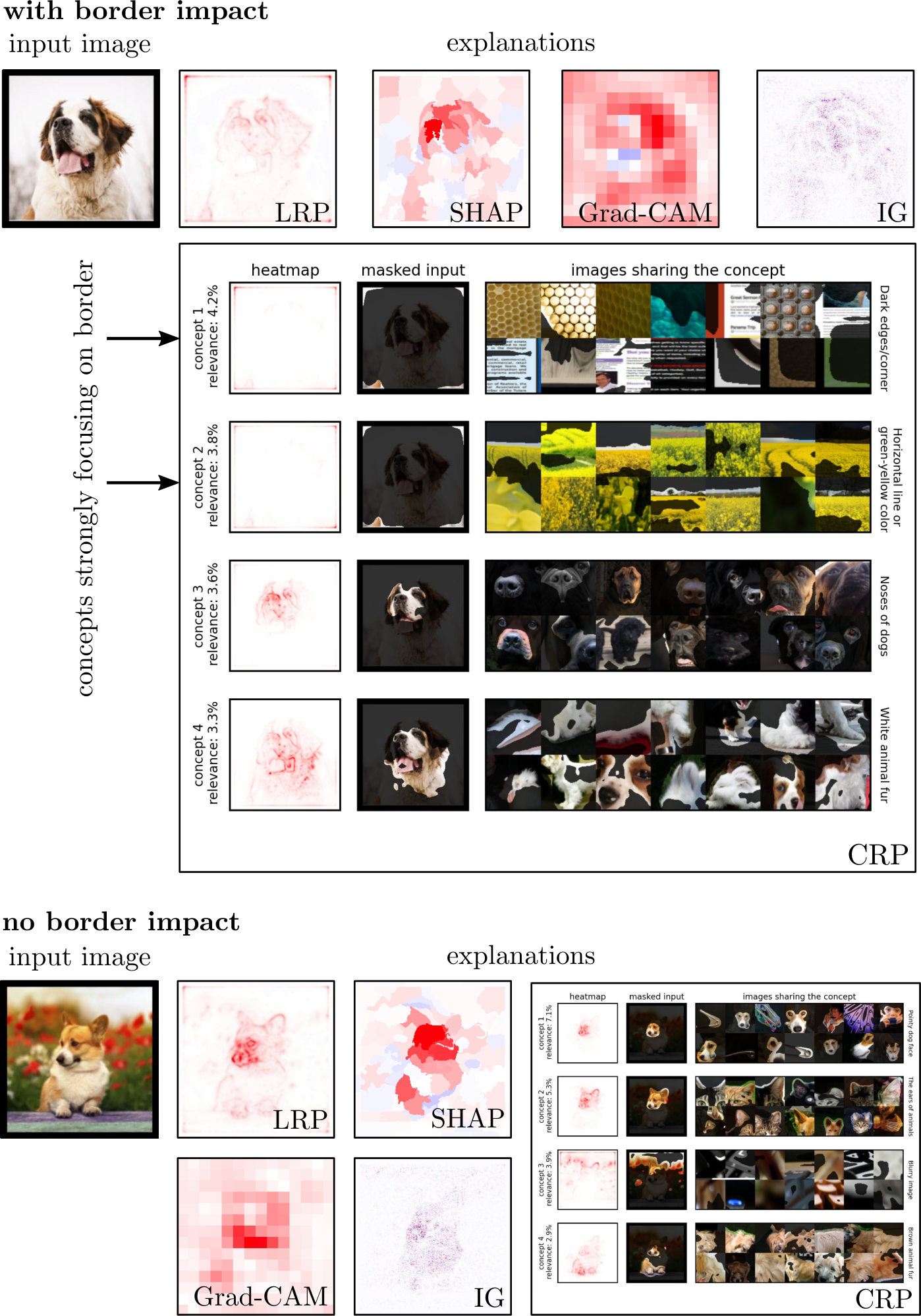
An example of resulting explanations is shown in Supplementary Figure 36 for all five methods with respect to a sample with (top) and without (bottom) a strong CH [70, 116, 7] impact on the target class. The black border width on the input sample is 9 pixels, while the overall image size was kept unchanged at 224 px224 px.
For LRP and Grad-CAM heatmaps, a shift from high relevance densities in the heatmap center to the border is visible, when the border has indeed a strong impact. On occasion, we observe a disproportionate amount of relevance on the border region for the model which has not been trained to utilize that feature at all. It is more difficult to see higher relevance on the border region for SHAP, as the border is part of a large number of super-pixels, where perturbations might not significantly impact the border artifact. Further, attributions from ig tend to be noisy, making it difficult to correctly interpret the explanations overall. CRP heatmaps show the four most relevant concepts in layer features.28 with corresponding heatmaps, relevance-masked input, masked reference images, and a suggested label for each concept. The label suggestions are generated in a first step using MILAN [55], which automatically generates natural language descriptions of masked reference images, and are further refined by the authors when necessary.
| Method | Accuracy (%) | F1-Score (%) | Confidence (%) | Clarity (%) |
|---|---|---|---|---|
| IG | ||||
| LRP | ||||
| SHAP | ||||
| Grad-CAM | ||||
| CRP (ours) |
The study participants were able to detect whether the prediction was impacted by the border most often using CRP explanations, as shown in Supplementary Table 3. CRP results in the highest accuracy of and F1-score of . Of the local methods Grad-CAM performs best with an accuracy of and F1-score of , and IG worst with accuracy and F1-score. It is to note, that random guessing would correspond to values of 50 %, indicating that the insight of IG explanations is limited in this study. Participants exposed to the IG explanations report the highest confidence — while at the same time performing worst in the primary task — followed by CRP . Regarding clarity of the explanations as perceived by the participants, the fine-grained attribution maps of IG and LRP receive the highest scores. CRP and RelMax interestingly result in the lowest reported clarity. These results are discussed in detail in the main manuscript in Section 3.4.
Appendix H Detailed Analysis: Clever Hans Detection and Quantitative Results
In the previous sections, we have qualitatively demonstrated the capabilities of our method for explaining machine learning predictions not only in terms of involved concepts, but also how those predictions can be broken down into corresponding concept-specific explanations again, and how this information may be visualized for exploring machine learning models and datasets.
In the following, we will move forward by showcasing how our achieved level of explainability may be used to interact with the model, e.g., by second-guessing its decision based on the features it has used, as revealed by Concept Relevance Propagation and its example-based explanations. First, starting with Section H.1 we give an answer to the question of how many concepts need to be observed and understood in order to comprehend a particular model decision given the hundreds of filters potentially encoding unique abstractions55 5 Fortunately, the answer is “not that many”!. This set of relevant concepts then allows for, e.g., entering a dialogue with the predictor and for asking “what-if” questions regarding its decision-making strategies. In Section H.2, we then investigate how a model trained on the ISIC 2019 skin lesion analysis dataset [32, 31, 130] reacts to the presence of clinically irrelevant concepts which have been discovered to be learned. In Section H.3 we show how our method can be used to first discover spuriously interesting (Clever Hans) concepts learned by the model, and then perform an explainability-based image retrieval in order to identify multiple classes affected by the same image artifact semantically, which however should be unrelated to the target labels. Finally, in Section H.4 we analyze the latent representations of relevance-based reference example sets and thus are able to identify sets of filters correlating in terms of activation, but differ in relevance for the purpose of encoding detailed differences between conceptually related ImageNet classes.
H.1 Quantifying the Foundation of Decision Making
In the previous sections, we have so far shown only a very limited amount of the most relevant concepts and examples as identified via relevance scores. For one, this is due to the static nature of this manuscript and its associated limitations66 6 Which arguably could be alleviated with interactive analysis tools, which are, at time of submission, under active development.. More importantly, with the usually high number of layers within an analyzed network and the hundreds of filters per layer, an exhaustive presentation of all explainability data per inference might quickly become overburdening to the observer. With those practical limitations in mind, we want to address the question of how much explanation is needed in order to sufficiently understand a particular inference of the model. Recent work on network compression and pruning has shown that contemporary neural network architectures often are highly over-parameterized and a large amount of filters can be removed without noticeable impact on the performance of the model [140, 138, 20]. The explicit representation of prototypes in some neural network architectures [27] has been exploited to remove spurious information from the decision making in a user-interactive fashion [45]. Based on this, we may assume that there exist neurons and filters which encode information irrelevant to a particular inference under analysis. To measure the extent of the (ir)relevance of explained and interpretable network elements, we perform an experiment based on the perturbation of a latent layer’s filters in accordance to their relevance scores, similar to the evaluation based on input perturbation described in [113]. We show that a large part of filters have indeed no impact on individual predictions, and only a small fraction of the available filters per layer do have a significant impact in favor or against the prediction made by the model, which need to be observed in order to understand the model’s reasoning.
Specifically, for a particular prediction we start with the computation of relevance scores, which are assigned to all layers, filters, and neurons of the model. Within a layer to be evaluated, we first rank the filters according to their (spatially sum-aggregated) relevance. Then, according to this ranking, we successively deactivate the filters in descending order (i.e., deactivating the most relevant representations first) by setting their activations to zero, and re-evaluate the model output. Since the initial output logits differ for each data sample, values are measured relative to the initial confidence values of the observed and explained model output. We refer to this process as “filter flipping” in accordance to the designation of “pixel flipping” from [13]. This procedure measures the impact a set of perturbed filters has on the decision outcome, and whether their relevance-based ranking is indicative of the model’s use of the therein encoded information during inference. The same procedure is repeated with an inverted filter ranking, i.e., perturbing the least relevant filters (potentially being relevant against the initial prediction outcome) first. Note that deactivating filters with negative relevance scores usually increases the prediction confidence, since negative relevance argues against the selected class, and removing them indirectly reinforces evidence for the selected class.
Supplementary Figure 37 (left) shows the distribution of ranked relevance scores per filter (averaged over 250 randomly drawn samples) within features.28 of a VGG-16 model, and Supplementary Figure 37 (center) the average cumulative sum of relevance over the rankings. Note that relevance scores attributed to filters tend to be power-law distributed, which holds true for both strong positive attributions, as well as strong negative attributions. This means that (on average) only a minority of filters are involved in per-sample inference, both in support and contradictory to the prediction outcome. In Supplementary Figure 37 (center) we can see that in order to observe 85 %, 90 %, or 95 % of the foundation of the model’s reasoning speaking for its prediction outcome (measured in terms of cumulative relevance), the user has to investigate and understand the concepts of the 58, 74 and 100 most important filters, respectively. Approximately 300 of the 512 filters in layer features.28 are not involved in predictions on average.
While having to look at “only” approx. 20% (which still are 100) of the layer’s filters to understand 95 % of the most relevant filters might indicate a high user workload, the results of the filter flipping experiment in Supplementary Figure 37 (right) do showcase that effectively, an even smaller fraction of the most relevant filters is responsible for the model’s decision confidence: We measured that in order to decrease the output confidence of the model relatively by 85 %, 90 %, or 95 % it is on average sufficient to deactivate only the 14, 16 or 20 most relevant filters, respectively.
In general, investigating individual neurons and their concepts is easiest if a small proportion of neurons are sufficient to explain most of any prediction. Observing the results regarding features.0 and features.14 it can be seen, that the earlier layers require a higher fraction of channels to analyze — compared to layer features.28. However, same as for layer features.28, flipping a few of the most relevant channels results in large drops regarding prediction confidence. The generally slower decay in confidence over most relevant flipped channels can be interpreted such that lower level concepts are not as class specific as more abstract representations later in the model, and as simpler features, such as edges or color gradients, are more likely to be shared among classes and exhibit a certain amount of redundancy and replacability in the lower layers. This is also supported by the earlier confidence decay when the least relevant channels are flipped. It is to note that for ResNet-like architectures, it should additionally be taken into account that relevance may be distribured unevenly among layers due to short-cut connections. ResNet models have high flexibility in how they allocate concepts within the model due to their short-cut connections. As a consequence, short-cut connections cause an additional non-uniform distribution of relevance between entire layers, not just neurons. This insight is for example exploited in neural network pruning [138]. Note, that the conservation principle of LRP (cf. [13]) inherited by CRP in theory guarantees that the total amount of relevance remains constant across parallel layers. The mean relevance flow throughout the ResNet architecture is shown in Supplementary Figure 38. Here, it is visible, that several layers do not contribute strongly to predictions, as they receive low attributions. This is further confirmed by a channel flipping experiment for a layer with high relevance (layer3.0.conv2 with a mean of over 50 % relevance) and one layer with low relevance (layer3.4.conv1 with a mean of less than 1 % relevance). The flipping of channels has a significant impact for layer3.0.conv2 on the model confidence. For layer layer3.4.conv1 on the other hand, the confidence is less affected, resulting in a mean confidence of still over 80 % after all channels are flipped. Investigating the flow of relevance through a model with, e.g., skip connections allows the user to distinguish which filters within a layer should be investigated, and whether this layer needs to be investigated at all, depending on whether the decision process has skipped the layer at hand.
We conclude that it is therefore possible to understand (or at least obtain a thorough overview about) the reasoning of the model in context of a particular sample by considering only a small fraction of all filters, since only the most important filters have a noticeable influence on the outcome. Further, it is to note that for simplicity, we assume in this study, that each filter encodes a learned concept on its own. This assumption will in general not hold, with multiple filters redundantly or in combination encoding highly similar or compound concepts in practice. A meaningful grouping or clustering of filters (see Section 3.3 in the main manuscript and Section H.4 for an outlook) can therefore further ease the task of interpreting machine learning explanations.
H.2 Investigating the Impact of (Clever Hans) Concepts
The methods proposed in this study allow to explore learned concepts and investigate their role in the decision process. Knowing which concepts exist allows to manipulate and test decisions. In the previous section, concepts are suppressed without taking their semantic meaning into account, and by setting whole activation maps to zero. In the following, we first insert and secondly replace distinct concepts in order to manipulate decisions. Specifically, we present two examples for the ISIC lesion classification task [130, 31, 32]. Here, different skin samples are classified into the diagnostic classes of melanoma (MEL), melanocytic nevus (NV), basal cell carcinoma (BCC), actinic keratosis (AK), benign keratosis (BKL), dermatofibroma (DF), vascular lesion (VASC), squamous cell carcinoma (SCC) and unknown (UNK). Using our approach, we are able to identify the filters responsible for encoding colorful band-aids polluting a significant fraction of the available samples [110], which is known to impact the inference of models trained on the dataset [7].

A CRP-based analysis shows that a VGG-16 model trained on the ISIC dataset has learned to use a band-aid concept for lesion detection. Locally, a higher-level channel (filter index 248 in features.28) for “colorful band-aid” and a lower-level channel (filter index 12 in features.0) for “yellow” can be identified and associated to the concepts, as is depicted in Supplementary Figure 39. The channel activation maps, as well as channel relevance heatmaps of the given sample support the finding, by consisting of large values in the spatial region of the band-aid. Further, these channels are most relevant for the decision, suggesting the identification of the source of Clever Hans behavior tied to these filters.

In the first experiment, the Clever Hans — i.e., the “band-aid” — concept, is inserted into 160 randomly drawn sample images which do not show band-aids. As shown in Supplementary Figure 40 (top), the “band-aid” expression is inserted in the prediction process via the higher-level layer features.28. To this end, the activation tensors are copied from a sample with a band-aid features to a sample without band-aid features. In order to only copy activations describing the band-aid concept, all activations are masked to overlap with the band-aid in the spatial dimension and then transferred to the target sample. Specifically, the activations (located in layer consisting of channels with spatial dimensions of size and ) for prediction of sample without a band-aid are replaced with activations from sample with a band-aid as
| (46) |
with the Hadamard product and the mask that spatially localizes the band-aid with values of one and zero else. The manipulation of can also be done gradually, controlled with parameter :
| (47) |
where controls the degree of localizedly blending in the band-aid expression. Performing the perturbation linearly, the change in class output as well as relevance for the top-5 strongest changing channels is depicted in Supplementary Figure 40 (top). For each channel, the four most relevant reference samples are shown. As is visible in the plots, a mean increase in output score for class 1 can be seen for band-aid insertion. The output score for class 0 most strongly decreases. This can in fact lead to a change in prediction outcome, as is shown in Supplementary Figure 41. Tracking relevance values of the individual channels shows, that channels with concepts supporting “band-aid” are growing in relevance with increasing perturbation. Specifically, channels with indices 248, 506 and 331 (activating for band-aids) receive more relevance on average when the band-aid concept is added.

In the second example, the “band-aid” concept is replaced in 25 band-aid-containing samples by a “skin” concept from a sample solely depicting skin. The manipulation is again performed in the higher-level layer features.28, as shown in Supplementary Figure 40 (bottom). Please refer to Supplementary Figure 42 for applications of the process to different layers. Regarding the skin concept, activations are averaged over the spatial dimension for the skin-only input image. Thereafter, these activations replace the latent space features during predictions defined by a mask covering the band-aid.

Specifically, the activations for the sample with a band-aid are gradually replaced with spatially averaged activations from a sample consisting of skin concept using parameter as
| (48) |
where controls the degree of blending in the skin expression and mask localizing the band-aid spatially with values of ones and zeros else. As is visible in the plots of Supplementary Figure 40 (bottom), the replacement of the band-aid concept leads to a decrease in prediction output for class 1. This manipulation again can lead to a change in prediction outcome, as is shown in Supplementary Figure 42. A decrease in the score for class 1 is expected, as in the first experiment the opposite happened when concept “band-aid” is inserted. Investigating the change in relevance of individual channels, we can see, that channels supporting a “band-aid” concept are decreasing in relevance. Channels such as (e.g., 248, 506 and 152), that previously gained relevance when “band-aid” was added, now lose relevance when the band-aid concept is replaced.

Besides showing additional individual manipulated samples, we show in Supplementary Figure 43 the band-aid insertion experiment for 160 randomly drawn samples for earlier layers, i.e., features.0 and features.10. Here, a similar effect as for features.28 can be seen: Adding the band-aid concept generally has the effect of increasing the output score of class 1. Further, channels corresponding to band-aid (e.g. in color for earlier layers or color and shape for later layers) grow in terms of relevance.
An ImageNet Use Case
In Supplementary Figure 20, we have seen, that the model uses several concepts that do not focus directly on the swimming trunks when detecting the respective class.

Supplementary Figure 44 illustrates how the model confidence changes when setting these Clever Hans artifacts to zero. The filter indices of potential Clever Hans artifacts are found by applying a local analysis on the skin of the surfer. The progressive masking or deactivation of whole latent filter channels encoding bare skin quickly decreases the model’s confidence in predicting class “swimming trunks”, verifying the Clever Hans behavior and its cause.
H.3 Explanation-based Image Retrieval for Clever Hans Assessment Beyond Class Boundaries
In this section, we demonstrate how Concept Relevance Propagation can be leveraged as a HITL solution for dataset analysis. In a first step, we will uncover another CH artifact, suppress it by selectively eliminating the most relevant concepts in order to assess its decisiveness for the recognition of the correct class of a particular data sample, similarly as in the previous section. Then, we utilize class-conditional reference sampling (cf. Section D.2) to perform an inverse search to identify multiple classes making use of the filter encoding associated concept, both in a benign and a Clever Hans sense.

In Supplementary Figure 45 we analyze a sample of the “safe” class of ImageNet in a pretrained VGG-16 BN model. Initially, we obtain an input attribution map highlighting a centered horizontal band of the image, where a watermark is located. If we take a closer look at layer features.30 and perform a local analysis (cf. Section B.3.2) on the watermark, we notice that the five most relevant filters are 454, 361, 203, 414 and 486. Visualizing them using ActMax as illustrated in Supplementary Figure 46, we conclude that they approximately encode for white strokes. Using RelMax instead (as also shown in Supplementary Figure 45), we gain a deeper insight into the model’s preferred usage and discover that the model utilizes the filters to detect white strokes in written characters.

To test the robustness of the model against the Clever Hans artifact, we successively set the activation output map of the 20 most relevant filters activating on the watermark to zero. In Supplementary Figure 45 (right), we record the decline of classification confidence of four classes with highest prediction confidence for this sample. From the graph, it can be inferred that the Clever Hans filters help the model in prediction, but they are not decisive for correct classification. Thus, the model relies on other potential non-Clever Hans features to detect the safe, verifying the correct functioning of the model in cases of samples without watermarks.
In an inverse search, we can now explore for which samples and classes these filters also generate high relevance. This allows us to understand the behavior of the filter in more detail and to find other possible contaminated classes. In Supplementary Figure 47 are the seven most relevant classes for filter 361 illustrated. Surprisingly, many classes including “whistle”, “mop”, “screw”, “mosquito net”, “can opener” and “safe” (among others) in the ImageNet Challenge 2014 data are contaminated with similar watermarks encoded via filter 361 of features.30 which is used for the correct prediction of samples from those classes. To verify our finding, we locate via CRP the source of the filters’ relevance wrt. the true classes in input space, and confirm that these filters indeed activate on the characters. This implies that the model has learned a shared Clever Hans artifact spanning over multiple classes to achieve higher accuracy in classification. The high number of contamination of samples with the identified artifactual feature could be explained by the fact, that watermarks are sometimes difficult to see with the naked eye (location marked with a black arrow) and thus slip any quality ensuring data inspection. The impact of this image characteristic can, however, be clearly marked using the CRP heatmap. Although the filter is mainly used to detect characters, there are also valid use cases for the model, such as for the puma’s whiskers or the spider’s web. This suggests that the complete removal of Clever Hans concepts through pruning may harm the model in its ability to predict other classes which make valid use of the filter, and that a class-specific correction [7] might be more appropriate.

H.4 Assessing Concept Similarity in Latent Space
So far throughout our experiments, we have treated single filters as functions assumed to (fully) encode learned concepts. Consequently, we have visualized examples and quantified effects based on per-filter granularity. While previous work and our own experiments suggest that individual neurons or filters mostly encode for a single human comprehensible concepts [142, 96, 104, 18, 24, 47]77 7 The cited literature concludes that the occurrence of poly-semantic units is rare for models trained on ImageNet., it can generally be assumed, that concepts are encoded by sets of filters: The learned weights of potentially multiple filters might correlate and thus redundantly encode the same concept, or the directions described by several filters situated in the same layer might span a concept-defining subspace [132]. Our proposed Concept Relevance Propagation readily supports the definition of concepts as sets of multiple features.
In this section, we now aim to investigate the encodings of filters of a given neural network layer for similarities in terms of activation and use within the model. For this purpose we present a simple but qualitatively effective method for grouping similar concepts in CNN layers: Based on the notation in previous sections, denotes a set of reference images for a channel in layer and the ReLU-activated outputs of channel in layer for a given input sample and all required network parameters W for its computation. Specifically, for each channel and its associated full-sized (i.e. not cropped to the channels’ filters’ receptive fields) reference samples we compute , as well as for all other channels , by executing the forward pass, yielding activation values for all spatial neurons for the channels88 8 Here, is an arbitrary choice, resulting from the common minimal size of available pre-computed reference sample sets for all filters.. We then define the averaged cosine similarity between two channels and in same layer as
| (49) | ||||
| (50) |
Note that we symmetrize in Equation (49) as the cosine similarities and are in general not identical, due to the potential dissimilarities in the reference sample sets and . Thus, measures the cosine similarity between filter and filter wrt. the reference samples representing filter . The from Equation (49) resulting symmetric similarity measures can now be clustered, and visualized via a transformation into a distance measure99 9 Note that normally, the output value of the cosine distance covers the interval , where for the two measured vectors are exactly opposite to one another, for 1 they are identical and for 0 they are orthogonal. In case output channels of dense layers are analyzed, i.e. scalar values, the range of output values reduces to the set , as both values are either of same or different signs, or at least one of the values is zero. Since we are processing layer activations after the ReLU nonlinearities of the layer, which yields only positive values for and . This results in , and a conversion to a canonical distance measure . serving as an input to t-SNE [131] which clusters similar filters together in, in our case, .
Supplementary Figure 48 shows an analysis result focusing on a cluster around filter from features.40 of a VGG-16 network with BatchNorm layers trained on ImageNet, representing facial features and fur patterns of house cats, with the most similar neighbor in terms of activatory behavior being filter 289, representing zoomed-in representations and facial features of tabby cats. Investigating the other neighboring filter of the cluster by following the spatial embedding and thus roughly their -similarity to filter 281, we can for one observe clear conceptual similarities of the filters as represented by their reference sample sets. Furthermore, we can observe a change in the nature of represented concepts: While filters 281 and 289 represent cat faces and fur pattern, as well as cat eyes in close-up view, the filters 160, 93 and 16 pick up on the concept of big eyes and respectively seem to represent large-eyed and flat nosed Persian cats and pug dogs in frontal view (filter 160), flat-faced animals with large black eyes and brown to white fur patterns (filter 93), and faces of animals of brown to gray fur with small black eyes (filter 15). After a larger step in embedding space, filters 454, 109 and 126 seem to further simplify the progression of animal face representations to black or large dots on uniformly colored round shapes (filter 454), to colorful shapes of lower complexity with dots (filter 109) to ultimately almost uniformly colored objects (filter 126), seemingly completing a transition to simpler and more abstract concepts starting at filter 281.

We discuss another analysis in Supplementary Figure 49 focussing on filter in features.40 of the same model, showing various types of typewriter and rectangular laptop keyboard buttons and roofing shingles photographed in oblique perspective, as well as round buttons of typewriters, remote controls for televisions, telephone keys and round turnable dials of various devices and machinery. Other than the concepts discovered in context of Supplementary Figure 48 and filter 281, the filters around filter 446 seem to cover different aspects of a shared “button” or “small tile” concept. The filters located in this cluster have been identified as similar due to their similar activations over the combined reference sample sets. Assuming redundancy based on the filter channels’ apparently similar activation behavior, the user could merge or cluster them to one encompassing concept, thereby simplifying interpretation by reducing the number of filters in the model. We therefore further investigate the filters 7, 94, 446 and 357 (all showing buttons or keys) in order to find out whether they encode a concept collaboratively, whether they are partly redundant, or whether the cluster serves some discriminative purpose.

We observe that the filters are most relevant for classes “laptop computer” and “remote control”. Consequently, we compute neuron activations and attribution scores for samples from both classes and observe the attributed relevance to those features when performing CRP wrt. the ground truth class output. See Supplementary Figure 50 for visualizations. Regardless of whether an instance from class “laptop” or “remote control” is chosen as input, the activation map across the observed channels is similar for each instance. The per-channel CRP attribution map however reveals that while all filters react to similar stimuli in terms of activations, the model seems to use the subtle differences among the observed concepts to distinguish between both classes they are most relevant for: For both class ‘‘laptop’’ and ‘‘remote control’’, buttons are striking and defining features, and all observed filters activate for button features. However, when computing relevance scores for class ‘‘laptop’’, the activating filters representing round buttons (filters 7, 94, and 446) dominantly receive negatively signed attribution scores, while filter 357 clearly representing typical keyboard button layouts receives high positive relevance cores. For samples of class ‘‘remote control’’, the computation of relevance scores wrt. their true class1010 10 or even the computation of CRP for samples from class “laptop” wrt. the class output for “remote control” yields almost exactly opposite attributions, indicating that filters encoding round buttons and dials (filters 94 and 7) provide evidence for class “remote control”, while the activation of channel 357 clearly speaks against the analyzed class visible in relevance attribution. In both relevance analyses, however, filter 446 receives no attributions, presumably as it represents a particular expression of both round and angular buttons which fits (or contradicts) neither of the compared classes particularly well. In fact, filter 446 is highly relevant for class “typewriter keyboard” instead.
In conclusion, we report that although several filters may show signs of correlation in terms of output activation, they are not necessarily encoding redundant information or are serving the same purpose. Conversely, using our proposed Concept Relevance Propagation in combination with the Relevance Maximization-based process for selecting reference examples representing seemingly correlating filters, we are able to discover and understand the subtleties a neural network has learned to encode in its latent representations

We present some additional interesting findings below. An additional t-SNE cluster example is shown in Supplementary Figure 51, visualizing filters spanning a conceptual subspace of water- , sea floor- and ground surfaces. Specifically, a total six channels forming a chain in the embedding space are displayed with their most relevant reference samples. Starting with channel 23 relevant for waves on the water surface seen from above, the next similar channel is channel 18 activating for a similar concept with differently colored water. Channel 48 corresponds to turquoise water above and below the surface. Thereafter, channel 99 and 325 are characterized by concepts describing corals and stones underwater. Eventually, channel 481 is used for grass and sand textures. This example illustrates how a semantic transition in terms of concepts can be seen discovered when analyzing the activations of latent neurons based on RelMax reference examples.


Another example of finding channels with similar concepts using t-SNE is shown in Supplementary Figure 52, where four channels can be found that are relevant for the recognition of legs of dogs and other animals (and objects). Here, the embedding allows splitting the space into several subspaces: Channels 328 and 282 are relevant for “bright-colored fur”, whereas channels 139 and 359 for “darker-colored fur”. On the other hand, channels 139 and 328 react for “long-haired fur” and channels 359 and 282 for “short-haired fur”. We might have identified a group of channels encoding the common concept of “legs” with degrees of freedom with regards to brightness and “leg volume”.

How these similar channels are differently used in predictions is shown in Supplementary Figure 53.
Appendix I Additional Experiment: Towards XAI for Fairness in ML
So far, we have demonstrated qualitatively how the reasoning process of a DNN can be understood using CRP and RelMax. Through a user study (see Section 3.4 in the main manuscript) we have further been able to quantify that our proposed set of novel techniques can be leveraged effectively to reveal shortcuts in a model prediction that exploit CH artefacts, on a conceptual and human-understandable level.
In this section we aim to demonstrate how our proposed techniques can be harnessed in probable real world applications, e.g., to expose discriminatory behavior against demographic groups in high-stake decisions potentially inflicting harm on individuals. This is specially relevant for applications with ethical and judicial implications, where decisions must adhere to moral and objective standards, as requirements set in governmental regulatory frameworks [48]. Examples for such discriminatory behavior include a recruiting tool for STEM job openings conjecturing that females are less qualified than men [36] or a software for rating a defendant’s risk of future crime systematically estimating African Americans having a higher risk than White American inmates [8]. The following experiment is merely intended as a brief excursion to the topic of XAI-supported fairness in ML. A detailed treatment is subject to future work.

For the purpose of this demonstration, we trained a VGG-16 model on the openly available Adience dataset [39] for male vs. female face classification (details on training are in Section L.1). Supplementary Figure 54 illustrates a concept atlas for a sample of class “female” that was correctly predicted. However, at the bottom part of the heatmap visualization to the left an aggregation of negative relevance scores is recognizable. Especially the collar of the person’s clothing receives negative relevance, indicating some visual evidence against the categorizaton of this sample into the output category “female”. If only the single heatmap visualization were to be considered for interpretation, a user might infer that the striking yellow color induces an unexpected model behavior. However, examining the first and fifth-most influential concept as shown in the Concept Atlas (channel 126 and 56 in Supplementary Figure 54) clarifies that the presence of the shirt collar as a particular clothing item, often related to the presence of a (bow) tie and male-looking chings, visual feature recognized and assessed as contradictory by the model.
Given this singular instance of inference and explanation, we are able to recognize that the model has learned a feature systematically, that encodes for collars of suits and shirts, which is responsible for the attribution of negative relevance due to its recognition as a non-female feature. Thus, conversely, the model has been exposed to over-associate the attribute “clothes with shirt collars” with the possible “male” outcome in this binary prediction problem, eventually causing discriminatory behavior in settings where an incorrect predictions due to a bias related to particular clothing items might have a negative impact on the well-being of individuals.
Supplementary Figure 55 shows another instance of a male face with long hair, which has been mis-predicted by the model as “female” based on a learned stereotype related to hairstyle. Provided explanatory information as shown in the figure, developers of machine learning models and datasets do have access to detailed information about systematic dataset biases as learned as well as abused by the analyzed model. One next reasonable step for developers could therefore be extension and diversification, as well as a more careful curation of the training data the model has been trained on, based on the insights from our XAI approach.

Appendix J Additional Experiment: Concept Analysis on Time Series Data
The application of explanation methods is not constrained to the image domain and has in the past seen utilization in numerous other data domains [114]. Also as long as the data domain can be meaningfully visualized in an interpretable way, obtaining concept-based explanations with CRP is possible.
Here, we present a use-case on how CRP can be utilized in a CNN model trained on Electrocardiography (ECG) arrhythmia data to verify the concepts used during inference and to open up the door to potential use-cases for scientific discovery in the future. A decisive factor for interpretability is choosing the right representation for the input domain. For example in sex classification on voice recordings a frequency representation is more advantageous in terms of XAI interpretability since here, pitches are easier to distinguish for the naked eye [19], than in time domain. For ECG data, the traditional time series representation is much more comprehensible for physicians, because they are familiar with this visualization on which characteristic markers have been defined in literature [78]. The original training data is provided by PhysioNet MIT-BIH Arrhythmia [87] and consists of ECG recordings from 47 different subjects, where each beat was annotated by at least two cardiologists. The work [61] reordered the dataset by isolating the ECG lead II data, splitting and padding beats into a fixed size of 150 at a sampling rate of 125 Hz and finally grouping all annotations into five different categories in accordance with the Association for the Advancement of Medical Instrumentation (AAMI) EC57 standard [12]. We train a model containing multiple layers of 1D-convolutional and densely connected layers. Details on the architecture and training procedure can be found in Appendix L.1. Assuming concepts are confined to single channels, we visualize again only single filters using RelMax. The attribution maps are projected to the input data domain and visualized as line plots. Similar to the image domain setting in Section C.4, we infer the receptive field at the hidden layers in order to identify and crop the most representative signal patterns for individual filters. In the future, this visual representation could be augmented by symbolic regression or other more precise mathematical descriptors of the concepts, such as the Romhilt-Estes score system [41].

The input sequence in Supplementary Figure 56 depicts the end of a premature ventricular contraction (PVC) or ventricular escape beat that was successfully detected by the model. A PVC is characterized by a wide QRS complex accompanied by a a left bundle-branch block pattern. In this case, a tall R wave and negative S wave, respectively, a high amplitude value followed by a valley is indicative [52, 4]. Investigating the concepts most relevant for classification, we perform two local analyses on two regions of interest. We can see that the filters used by the model correspond to the input pattern at the chosen region. The attribution graph, depicting the relevance flow from higher layer concepts in layer features.6 to lower level concepts in layer features.0, illustrates how filter 1 is composed of two concepts corresponding at one hand to the upper decline and secondly to the low voltage valley. Channel 41 in features.6, responsible for detecting a high amplitude followed by a valley, is most relevant for the PVC category on average, indicating that the model correctly identified the distinctiveness of a PVC1111 11 Time dependency between beats plays also a role that is not apparent from the shown visualization.. In the same way, XAI has the potential to be used for scientific discovery, e.g., for revealing previously unknown characteristics of known phenomena [37, 101, 129]. However, the filter corresponds only to 4.4 % of total absolute relevance representing a fraction of the decision process.
In summary, we demonstrated the applicability to data in non-image-domains and we have taken the first steps towards testing models for plausibility and scientific discovery.
Appendix K Challenges and Future Work
While we qualitatively show in the paper, and quantitatively verify in the conducted user study (Section 3.4 in the main manuscript), that our CRP- and RelMax-based explanations are able to deliver more informative explanations compared to their attribution-only counterparts, there are still certain difficulties to overcome in future work. While some of those difficulties are related to the choices a user can (and has to) make when using our approaches, others may be solved algorithmically in the future.
K.1 Interpreting Reference Samples
As it is common practice with Feature Visualization methods in the literature (see Section A.2), reference samples are typically intended to be interpreted by the human user. We address certain shortcomings of the in related work widely used ActMax approach for selecting or generating reference examples, e.g. the task-independency of activation scores or activations “overshooting” beyond for the model useful levels. While our proposed RelMax measure addresses some of these concerns, it might still by very challenging to uncover the “gist” of a learned latent encoding as represented by a limited set of either not very, or even too varied reference examples (see Section D.2). The shown examples might at times simply be too abstract to be palpable with human intuition (see Section E.4), as there is no guarantee that a neural network will categorize the world and abstract its concepts the way we humans prefer. With RelMax we complement the widely used concept “stimulation” technique embodied by the many variations of ActMax with a measure for concept “utility”. Nonetheless, we argue that an incorporation of constraints towards “image simplicity” [80] or measures related to concept “clarity” [93] might be beneficial to the human interpretability of the models’ internal representations.
In general, the degree of human-interpretability can vary depending on the model architecture, training procedure (training steps, dataset size, etc), or from layer to layer. In our experience, concepts are more distinct in models with higher accuracy as well as in VGG-like models compared to, e.g., ResNet models. Some models may rely on more neurons than others to encode similar concepts, potentially increasing robustness and redundancy. Such an effect can occur with, e.g., dropout layers [146] used during training. With multiple filters redundantly or in combination encoding highly similar or compound concepts, a meaningful grouping or clustering of filters (see Section 3.3 in the main manuscript and Section H.4 for an outlook) may therefore further ease the task of interpreting machine learning explanations.
Contemporary work such as Concept Whitening [28] tries to increase the clarity and distinctness of concepts with a specialized training procedure by aligning neuron activations to concepts predefined by humans. MILAN [55] on the other hand, approaches the interpretation of latent encodings in a data-driven way by training an image-to-text model applicable to reference images in order to provide suggestions for language descriptors, as an option to provide more objective interpretations of concepts, instead of potentially per-user unique readings.
Since CRP and RelMax are out-of-the-box applicable to (almost) any model without imposing constraints on the training process, the data and label availability, or the model architecture, the aforementioned techniques or other future concept enhancing methods can be integrated within the CRP framework.
K.2 Degrees of Freedom in Glocal Analyses and the Effects User Workload
One important point to consider when it comes to the application of XAI is the workload imposed on the user. With the exponential amount of parameters to consider and information to process with glocal explanations compared to traditional local approaches, we see this as a major issue when it comes to the effective utilization of this kind of XAI feedback. In the following we will briefly highlight some of the encountered issues with glocal XAI, and how to potentially mitigate them in future work.
Where to start a glocal analysis?
Compared to local methods such as LRP or IG, for instance, CRP explanations offer a much higher potential for model understanding by providing the possibility to interpret how concepts are used in all layers of the model architecture. However, the large number of layers and neurons to investigate can be overwhelming at first, which, e.g., reflects in the relatively low “clarity” scores of CRP & RelMax in our user study (see Supplementary Note G), despite the methods’ leading success in informing the user to solve the study’s primary task.
We find that a good starting point for the investigation of concept-based explanations usually are higher level layers, as they typically are comprised of more specialized and class-specific, as well as abstract concepts. From then on, a hierarchical analysis of concept composition might be followed, as it has been briefly introduced in this work (see Supplementary Figure 3d in Section 3.1 of the main manuscript), yet not explored to the full extent. Still, with the expansive amount of potential interactions of encodings, manual analysis might become infeasible quickly, and an algorithmic approach to present a condensed explanatory report (at least as an initial summary) to the user might be required.
The pain of choosing the right attribution variant
In theory, LRP— and therefore also CRP— can be applied to any model which can be presented in form of a directed acyclic graph, which includes all common DNN architectures. However, since the computational steps in different architecture types may change significantly, purposed implementations of LRP-rules and model canonizations (see Section L.2) may have a positive impact on the quality of the explanations obtainable [65, 90, 54], and very well-tuned parameterizations for LRP and in extension CRP might be desired in order to optimize the expressiveness of the glocal explanations as much possible. Hence, Arras et al. [10] specifically adapt LRP to analyse LSTMs, while Chereda et al. [29] and Schnake et al. [115] modify LRP for Graph CNNs. Despite research endeavors such as zennit [6], at the time of publication, no all-encompassing library exists that implements all LRP variants exhaustively. Alternatively, other backpropagation-based attribution methods can easily be utilized as well within the broader scope of the CRP framework, yielding different measurements on a model’s inference process and thus extending the option space of the user, but also the agony of choice.
What to investigate on a concept level?
Next to the framework-specific choice to make where (within the model) to start the analyses, and how to assess feature importance via the choice of an attribution method, there is the parameter-dependent choice of what to analyze. We have proposed the RelMax quantity measuring “utility” complementarily to “feature stimulation” as measured by ActMax. While alternative measures such as a potential Sensivity [88, 14] Maximization measuring the volatility of the model around a given reference example, the wealth of (the product space of) choice here again might become overwhelming quickly, even if one considers that each measure usable for procuring reference examples may generate an output representing a single distinct aspect of an ML model’s behavior. That even the restricted glocal explanations we have shown to the participants of our user study can be demanding already is apparent from the study results: even though the presented explanations based on CRP and RelMax have been demonstrated to be most effective for the goal of understanding model behavior, they perform worst in terms of user-reported explanation clarity.
In the XAI research domain, there is an emerging understanding on the criticality of objectively measuring different aspects of explanation quality quantitatively [54, 3]. While this is currently still difficult terrain, at times under-specified and overall not well-explored even when dealing with explanations on a single-heatmap-level, quantitative measures to algorithmically tune glocal explanations might be an option to optimize the user-presented information for optimal technical parameters, to be at the same time as informative concise as possible.
Appendix L Datasets, Models and Implementation
In the following, we provide a brief overview over the various datasets and models used throughout our experiments. Furthermore, we provide technical details and recommendations regarding our Concept Relevance Propagation approach.
L.1 Datasets and Models
ImageNet
Caltech-UCSD Birds 200
We fine-tuned a ResNet34 [53] pretrained on ImageNet on the Caltech-UCSD Birds 200 [135] dataset. Images are normalized with ImageNet values1212 12 Subtraction of mean values [0.485, 0.456, 0.406], followed by a normalization of standard deviation values [0.229, 0.224, 0.225] over the red, green and blue color channels respectively, as per specifications at https://pytorch.org/vision/stable/models.html.. Further, Gaussian noise (zero mean, standard deviation of 0.05), random horizontal flips (probability of 0.5), random rotation (up to 10 degrees), random translation (up to 20 % in all directions) as well as a random scaling (between 80 and 120 %) is applied for data augmentation. After 100 epochs of training using Stochastic Gradient Descent (SGD) with a value for momentum of 0.9 and weight decay of 1e-4, we achieved 76 % top-1-accuracy on the test set.
ISIC 2019
We employ the VGG-16 model with pretrained weights on ImageNet from the PyTorch model zoo to train on the ISIC 2019 dataset. The model is trained over 100 epochs, using an SGD optimizer with a learning rate of 0.001, momentum 0.9 and batch size of 32. ISIC 2019 does not offer a pre-defined labeled test set. Therefore, 10 % of the original training set is split off in order to evaluate the model’s performance. The model achieves a final test accuracy of 82.15 %.
Adience
We fine-tuned two VGG-16 models without BatchNorm layers pretrained on ImageNet on the Adience dataset [39] for age estimation as well as sex prediction. For training, folds 0,1,2 and 3 were selected and fold 4 was used as as a test set. Images are normalized with ImageNet values and linear transformations were applied as augmentation techniques. After training for 10 epochs with the Adam optimizer and a batch size of 32 with a learning rate of as well as standard hyperparameter values in the PyTorch library, we achieved a top-1-accuracy of 51.0 % (age estimation) and 93.6 % (sex prediction) on the test set.
PhysioNet MIT-BIH Arrhythmia
The original training data is provided by PhysioNet MIT-BIH Arrhythmia [87] and consists of ECG recordings from 47 different subjects, where each beat was annotated by at least two cardiologists. The work [61] reordered the dataset by isolating the ECG lead II data, splitting and padding beats into a fixed size of 150 at a sampling rate of 125 Hz and finally grouping all annotations into five different categories in accordance with the Association for the Advancement of Medical Instrumentation (AAMI) EC57 standard [12]. Preprocessing steps include subtracting the mean value of 0.2115 and standardizing by dividing with 0.2462. As optimizer, RMSprop [56] with a learning rate of 1e-4 and weight decay of 1e-6 were chosen. Since the data set is unbalanced, we used cross entropy loss with class balancing. We trained the model for 25 epochs and achieved on the test set an average accuracy of 89 %. Deep Residual CNN models achieve in comparison 93.4 % average accuracy [61]. The model consists of three feature extraction blocks, each composed of a 1D-Convolutional layer with 64 channels and kernel size 7, followed by a ReLU non-linearity and a 1D-Max-Pooling layer with kernel size 3 and stride 2. After feature extraction, a 1D-Average-Pooling layer with kernel size 7 and a flatten operation direct the activations into a regression head. The regression head consists of two linear layers with 64 and 32 neurons as well as a ReLU non-linearity. Finally, a linear output layer with 5 neurons concludes the architecture.
Fashion-MNIST
Human Study ImageNet Models
In the human study presented in Section 3.4, two fine-tuned VGG-16 models pretrained on ImageNet are used. Both models are trained for one epoch using a learning rate of with the Adam optimizer and a batch size of 32. Images during training are resized to 256 px for the smaller edge, followed by a center crop to 224 px224 px size and normalization with means of [0.485, 0.456, 0.406] and standard deviations of [0.229, 0.224, 0.225] over the red, green and blue color channels respectively. Finally, for the first model, all images are padded with a black border of 10 px width and again re-scaled to 224 px224 px size. For the second model, only images from 30 randomly chosen classes are displayed with the border artifact during training.
Image Licenses
The license to re-use and reproduce have been granted for the images shown in the figures of this supplementary material and the main manuscript to the authors by the respective copyright holders by iStock, Shutterstock, Pixabay and Pexels.
L.2 Implementation Details for Concept Relevance Propagation
Distribution Rules
In this work, we compute CRP attribution scores for ResNets and VGG-16 models using the recommended [65] composite LRP-rule1313 13 read: ”epsilon-plus-flat” rule after model canonization steps applied [58, 50, 90] as implemented in the zennit [6] package for PyTorch [98]. The LRP -rule is defined as
| (51) |
where with inputs from the lower layer and weights of the linear layer with outputs . It ensures that each neuron receives the attribution value, that it contributed to the output. The added stabilizes the division of the denominator. Note that for this purpose, the definition of the sign function is altered such that . The -rule is in ReLU networks highly similar to the multiplication of the input times its gradient wrt. the output [65], but not identical, leading to different attribution maps [90]. These attribution values for different predictions can now, in principle, be compared. However, due to its similarity to gradient-based attribution computation, the LRP -rule may result in noisy attributions in very deep models, where gradient shattering and noisy gradients appear[16]. Thus, the computation of the LRP -rule may not result in meaningful attributions in models with a high number of layers and ReLU activations. An alternative approach is to combine multiple propagation rules, so-called composite rules, which result in attributions that are less influenced by a noisy gradient: the LRP-rule is an established best practice [65, 84] to keep LRP attribution maps informative, readable and representative while combating gradient shattering effects. Here, applying the LRP--rule to the first convolutional layer smoothes the attribution map in input space and yields an invariance against input normalization effects. The LRP--rule, on the other hand, operates on the remaining convolutional layers and LRP -rule is utilized in standard MLP layers. The LRP--rule is defined as
| (52) |
Using the -rule, relevance of upper-level neuron is equally distributed to all connected lower-level neurons disregarding any influence of learned weights or input features. The LRP--rule is given as
| (53) |
by only taking into account positive contributions with .
Initialization
The calculation of an attribution map starts with an initial relevance value at the output neuron. A meaningful and canonical choice is the model output activation of the neuron representing the class of interest to be explained. All intermediate relevance values are then proportional to the initial relevance value, since LRP is a layer-wise linear distribution process, cf. Equation (24). We recommend to start propagation with the output values as they are, i.e., , for an output (set) of choice. Thus, the relevance of all neurons is proportional to the confidence of the model prediction. Note that a selection of more than one, output neuron to initialize the might lead to unclear attribution-based explanations, as shown in Supplementary Figure 1. As a result, when ranking the samples of a dataset for representing the concept of a filter, RelMax will give preference to samples that the model predicted with highest confidence. This behavior is advantageous when calculating class-conditional reference samples or when the original dataset is not expanded with additional datasets as demonstrated in (see Section D.2).
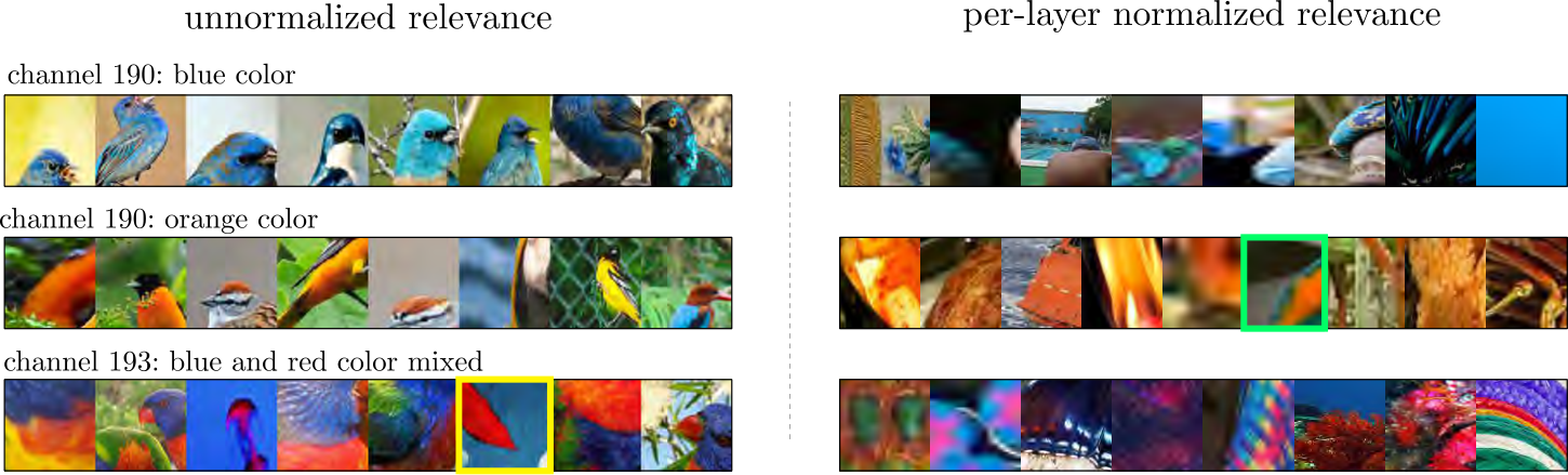
Canonization
Since rule-based attributions, such as LRP and CRP, are not implementation invariant, canonization restructures a model into a functionally identical equivalent of alternative design to which established attribution rules can be applied in an improved manner. Canonization efforts usually concentrate on replacing the BatchNorm layer [58, 50] or the handling of skip connections [21]. By merging BatchNorm layers into a neighboring linear layer, significant improvements in terms of explanations can be achieved [90].
Per-layer Relevance Normalization
We generally recommend starting the relevance backpropagation process with the output of a network element. However, when reference datasets are extended in order to gain additional perspectives on the concepts to be understood, out-of-distribution data (or data the model has not sufficiently fit to) will produce low output confidences which serve as low initial relevance values. This will result in the added reference data from alternative source to not be ranked highly as meaningful representations for latent concepts. In order to be in this case independent of the model confidence of individual predictions, the relevance attributions with condition can be normalized at each layer as
| (54) |
Thus, individual attributions are first divided by the absolute sum of relevances at layer to ensure that each attribution is bounded in . The concept importance becomes independent of the output of the model, while maintaining class-specificity. This procedure facilitates the comparison of concept importance for different samples during RelMax, if the original dataset is expanded with additional, external datasets. In our case, ImageNet images are fed into a model trained for bird categorization only. These ImageNet images will then be considered more frequently as representations for latent concepts with per-layer normalization than without layerwise normalization. It is to note, that class conditional relevance computation without ground truth labels has to be applied with caution, because the natural filter functionality, that the model confidence provides, is lost via per-layer relevance normalization. However, if (matching) ground truth labels are available, class conditional relevance could be computed for true labels only instead.
The qualitative difference of reference samples selected using RelMax with and without per-layer relevance normalization is illustrated in Supplementary Figure 57. Here, layer layer.3.0.conv1 of a pretrained ResNet34 model trained on Caltech-UCSD Birds 200 is analyzed. The dataset is extended with additional ImageNet samples to increase reference sample variety. Supplementary Figure 57 (left) depicts reference samples selected without per-layer relevance normalization, i.e., favoring samples that achieve highest model confidence. As a consequence, samples that belong to the original training data are visualized more often, illustrating how the filter is actually utilized. On the other hand, Supplementary Figure 57 (right) depicts reference samples selected with per-layer relevance normalization, i.e. selecting samples independent of model confidence. As a result, samples outside the training data are shown more often, providing examples more focused on the concept itself and with less distracting information increasing model output confidence in context of other concepts. The choice of applying layer-wise relevance normalization provides the option for an additional perspective on the visualized concept representations
Practical Implementation
The library zennit [6] was used to perform the experiments. It takes advantage of PyTorch’s autograd module to compute gradients in computational graphs. zennit modifies the backpropagated gradient in such a way that they are replaced by attribution values for CRP instead. We provide a zennit-based open source package for CRP and RelMax computations for PyTorch and Python at https://github.com/rachtibat/zennit-crp.