User Association and Multi-connectivity Strategies in Joint Terahertz and Millimeter Wave 6G Systems
Abstract
Terahertz (THz) wireless access is considered as a next step towards sixth generation (6G) cellular systems. By utilizing even higher frequency bands than 5G millimeter wave (mmWave) New Radio (NR), they will operate over extreme bandwidth delivering unprecedented rates at the access interface. However, by relying upon pencil-wide beams, these systems will not only inherit mmWave propagation challenges such as blockage phenomenon but introduce their own issues associated with micromobility of user equipment (UE). In this paper, we analyze and compare user association schemes and multi-connectivity strategies for joint 6G THz/mmWave deployments. Differently, from stochastic geometry studies, we develop a unified analytically tractable framework that simultaneously accounts for specifics of THz and mmWave radio part design and traffic service specifics at mmWave and THz base stations (BS). Our results show that (i) for negligible blockers density, bl./, the operator needs to enlarge the coverage of THz BS by accepting sessions that experience outage in case of blockage (ii) for bl./, only those sessions that does not experience outage in case of blockage need to be accepted at THz BS, (iii) THz/mmWave multi-connectivity improves the ongoing session loss probability by depending on the system parameters.
Index Terms:
Terahertz, 5G, 6G, millimeter wave, outage, micromobility, blockage, user associations, multi-connectivityI Introduction
Similarly to millimeter wave (mmWave) New Radio (NR) systems providing capacity boost for cellular infrastructure in places with high traffic demands [1], terahertz (THz) access systems are expected to be utilized in locations with the need for extraordinary data rates [2]. However, in addition to extreme capacity, these systems bring several unique challenges to system designers, making efficient deployment and utilization of such systems a complex task.
The propagation and link layer specifics of THz communications have been studied fairly well so far. Similarly to mmWave systems, THz communications are subject to blockage phenomenon [3]. In addition to higher free-space propagation losses, THz propagation is also much heavier affected by atmospheric absorption as compared to mmWave band [4]. Finally, by relying upon extremely directional antenna radiation patterns with half-power beamwidth (HPBW) of the main lobe approaching , these systems may suffer from frequent outages due to UE micromobility [5, 6]. These specifics make THz links highly unreliable requiring natural support from other technologies to ensure session service continuity at the THz air interface.
Future THz wireless access systems will target the support of rate-greedy applications such as virtual/augmented reality (VR), 8/16K streaming, holographic telepresence that are inherently sensitive to outages [7]. To improve session continuity of applications running over inherently unreliable wireless technologies, 3GPP has recently proposed the multi-connectivity functionality [8]. According to it, UE is allowed to maintain two or more active connections to nearby base stations (BS) of the same or different radio access technologies (RAT), referred to as inter- and intra-RAT multi-connectivity, respectively. The intra-RAT multi-connectivity has been studied in detail in context of mmWave 5G NR systems [9, 10, 11, 12], where it was shown to drastically improve outage performance of UEs. However, the limited coverage of prospective THz BSs as compared to mmWave NR BSs will require very dense deployments to efficiently utilize intra-RAT multi-connectivity.
To improve reliability of user sessions in future 6G THz/mmWave deployments, inter-RAT multi-connectivity operation can be utilized. However, the only other RAT having comparable albeit much smaller resources at the air interface is 5G NR operating in mmWave band. In spite both technologies target similar type of rate-greedy outage-sensitive applications, there is an inherent capacity mismatch between technologies. Thus, one needs to account not only for the radio specifics but for details of the resource allocation process at BSs. Furthermore, differently from the joint usage of microwave (Wave) and mmWave technologies [13, 14], both mmWave and THz RATs are subject to blockage events that require careful design of user association strategies. Finally, THz RAT is also affected by UE micromobility. To the best of the authors’ knowledge, there are no studies assessing the use of inter-RAT multi-connectivity in 6G THz/mmWave deployments.
In this paper, we fill the abovementioned gap by evaluating and comparing performance of user association schemes and multi-connectivity strategies in joint THz/mmWave radio access networks. Contrarily to the previous studies of user associations in heterogeneous access systems, we explicitly account for not only radio part specifics of considered technologies including propagation, dynamic blockage and micromobility effects but the traffic service process at mmWave and THz BSs. The performance of the considered user association schemes and multi-connectivity strategies are assessed and compared based on the user- and system-level metrics including new session loss capabilities, ongoing session loss probability as well as system resource utilization.
The main contributions of our study are:
- •
a mathematical framework based on stochastic geometry and queuing theory allowing for unified characterization of association schemes and multi-connectivity strategies by accounting for both radio and service part specifics;
- •
numerical analysis of user association schemes and multi-connectivity strategies for THz/mmWave deployments;
- •
numerical results showing that: (i) there is trade-off between new and ongoing session loss probabilities that depends on the choice of association and multi-connectivity strategy, (ii) the choice of the optimal association scheme mainly depends on the blockers density, (iii) tolerance of applications to short-term outages caused by antenna misalignment may greatly improve user performance, and (iv) intra-RAT multi-connectivity improves the ongoing session loss probability by approximately .
| Notation | Description |
|---|---|
| mmWave and THz carrier frequencies, Hz | |
| mmWave and THz BS bandwidths, Hz | |
| requested rate of sessions, Mbps | |
| intensity of session arrivals, sess./s/m2 | |
| number of THz BSs in the coverage of mmWave BS | |
| density of blockers, bl./m2 | |
| mmWave BSs coverage radius, m | |
| THz BS coverage radius, m | |
| mmWave BS height, m | |
| blocker speed (m/s), height (m), and radius (m) | |
| UE height, m | |
| mmWave BS emitted power, W | |
| thermal noise power, dBi | |
| mmWave BS antenna array gain | |
| mmWave UE antenna array gain | |
| mmWave propagation coefficient | |
| mmWave path loss exponents | |
| mmWave shadow fading in blocked state, dB | |
| cell edge outage probability at mmWave/THz BS | |
| SINR outage threshold, dB | |
| STD of the shadow fading in LoS blocked state, dB | |
| mmWave BS height, m | |
| THz BS emitted power, W | |
| THz BS antenna array gain | |
| THz UE antenna array gain | |
| THz propagation coefficient | |
| THz path loss exponents | |
| mmWave and THz interference margins, dB | |
| absorption loss, dB | |
| absorption coefficient, m-1 | |
| THz BS height, m | |
| THz BS antenna configuration, el.el. | |
| THz UE antenna configuration, el.el. | |
| mmWave BS antenna configuration, el.el. | |
| mmWave UE antenna configuration, el.el. | |
| THz array switching time, s | |
| THz beamalignment duration, s | |
| outage tolerance time of applications, s | |
| mean service time of sessions, s | |
| session resource requirements pmfs | |
| blockage intensity at mmWave BS, bl./s | |
| outage intensity caused by micromobility events/s | |
| outage intensity caused by blockage, events/s | |
| outage fraction for on-demand/periodic alignment | |
| outage for on-demand/periodic beamalignment, s | |
| time to outage due to micrimobility, s | |
| pdf of time to outage in presence of micromobility | |
| periodic beamalignment interval, s | |
| connection recovery intensity for blockage, events/s | |
| connection recovery intensity for micromob., events/s | |
| probability that the UE is assigned the MCS | |
| THz UE association probability | |
| random displacements processes over - and -axis | |
| yaw and pitch rotational mobility processes | |
| antenna array HPBW, ∘ | |
| array maximum and 3 dB points, ∘ | |
| blockage probability at distance | |
| number of NR MCSs |
II Related Work
System-level performance analysis of future 6G THz systems has been mainly studied so far by utilizing stochastic geometry approach. The studies mainly concentrated on characterizing impairments produced by blockage and micromobility as well as on the techniques utilized to mitigate them. Specifically, the authors in [15, 16] characterized interference and signal-to-interference plus noise ratio (SINR) at UEs by accounting for blockers density and directional antennas. Further, studies extending those works to deployment specifics have been published, see Shafie et al. [17] for 3D, Wu et al. [18] for indoor deployments, etc. Recently, the authors also investigated the effect of 3GPP multiconnectivity in dynamic blockage environment in [19]. These results have been further extended to account for micromobility in [20]. In both studies, the authors concentrate on capacity and outage probability showing that multiconnectivity improves both metrics.
Much less is known about system-level performance of joint operation of mmWave/THz systems. Among few others, is the study in [21], where the authors formulated the optimization problem of determining user associations in joint mmWave/THz systems to improve UE throughput in these systems. Another similar study targeting associations in these systems is [22], where a coexisting Wave and THz system has been considered. By utilizing system-level simulations heuristic UE associations algorithms have been proposed. However, similarly to THz-only systems, the abovementioned studies mainly concentrate on elastic traffic patterns.
The main rationale for utilizing mmWave and THz systems jointly is the type of traffic they target. By providing extreme amount of resources at the air interface both RATs target rate-greedy non-elastic applications such as AR/VR, 8/16K streaming, holographic telepresence [7]. One of the inherent properties of joint mmWave/THz systems is that both of them are subject to dynamic blockage while THz systems may further be affected by micromobility. There are few studies published to date targeting non-elastic traffic in mmWave only systems [12] or mmWave/Wave systems [14] with multiconnectivity support. Among other conclusions, [14] shows that temporal offloading of rate-greedy connections to Wave systems leads to detrimental effects in terms of UE having Wave interface only, while [12] illustrates that mmWave system alone may still lead to non-negligible loss probability of sessions accepted to service.
The conventional analysis tool utilized in the past – stochastic geometry – is no longer sufficient alone for mmWave/THz systems as it inherently assumes elastic traffic. To make conclusions on the performance characteristics of the session service process in joint mmWave/THz systems we need to take into account not only the specifics of the radio part and stochastic factors related to the randomness of channel and UE locations, but the traffic service dynamics at BSs by joining the tools of stochastic geometry and queuing theory.
III System Model
In this section, we introduce our system model. We define the deployment, dynamic blockage, propagation, antenna, beamalignment, and micromobility models, and then complement them with the resource allocation and traffic assumptions. Finally, we introduce the user associations and dynamic multi-connectivity assumptions as well as the metrics of interest. The notation used in this paper is provided in Table I.
III-A Deployment Model
We assume a mature phase of mmWave NR market penetration by considering a well-provisioned mmWave BS deployment. We tag and consider an arbitrarily chosen circularly-shaped service area of mmWave BS with radius , where is such that no outage happens at the cell boundary in line-of-signt (LoS) blocked state, see Fig. 1. This radius is determined in Section V by utilizing the set of NR modulation and coding schemes (MCS, [23]) and propagation model defined below.
In the coverage area of mmWave BS an operator is assumed to deploy THz BSs. The geometric locations of these THz BSs are uniformly distributed. The maximal feasible coverage radius of these THz BSs is determined by the propagation model introduced in what follows, while the actual coverage depends on the user associations schemes discussed below. The heights of mmWave and THz BSs are constant and given by and . The carrier frequencies are denoted by and , while the available bandwidth – by and . In what follows, we assume that . The rationale behind this assumption is that the bandwidth to cellular systems roughly increases by ten times in each generation and is expected to reach 20+ GHz for 6G THz access. Accounting for limited coverage areas and the rates of forthcoming applications (e.g., 10-40 Gbps for XR/VR, [24]) the capacity of these systems will be sufficient to maintain thousands of simultaneous sessions. However, the proposed framework can also be modified to account for finite capacities at THz BSs [12].

III-B Blockage, Antenna, and Propagation Models
III-B1 Blockage Model
We assume that the LoS between the mmWave/THz BS and the UE can be blocked by users. To this aim, we adopt a dynamic blockage model. According to it, pedestrians, acting as blockers, move by following a random direction mobility model (RDM, [25]). The speed and run length are m/s and an m, respectively. The density of pedestrians is units/m2. We model them by cylinders with radius and height . The height of blockers is assumed to be , , where is the constant height of UEs.
III-B2 Antenna Model
At both BS types we assume planar antenna arrays. By following to [26, 15], we use the cone antenna model, where the width of the beam coincides with the radiation pattern’s half-power beamwidth (HPBW). The mean gain over HPBW is known to be [27]
| (1) |
where is the number of antenna elements.
THz BSs and UEs are equipped with arrays having and elements, respectively. Similarly, mmWave BS and UEs are equipped with arrays having and elements, respectively. The array’s HPBW, , is found as , where is the radiation pattern’s maximum, are the 3-dB points. In practice, one may also use approximation [27].
III-B3 MmWave Propagation Model
To represent the mmWave path loss we utilize 3GPP Urban Micro (UMi) Canyon-Street propagation model defined in [28], i.e.,
| (2) |
where is the UE-BS distance measured in meters while is the carrier frequency in GHz.
The model in (2) can be converted to the linear scale, to the form , where and are the some coefficients. Introducing and corresponding to LoS blocked and non-blocked states, we have
| (3) |
Thus, the value of SINR at the mmWave UE can be written as a weighted function of SINRs in blocked and non-blocked states, as follows
| (4) |
where is mmWave BS emitted power, and are the mmWave BS and UE gains, is the bandwidth of mmWave BS, is the interference margin, is 3D UE-BS distance (Fig. 1) and is the blockage probability given by [29]
| (5) |
where is the intensity of blockers, and are the blockers’ radius and height, is the height of UE, is the height of mmWave BS.
III-B4 THz Propagation Model
The principal difference between mmWave and THz propagation models is presence of atmospheric absorption [4]. By utilizing the results of [15], the absorption loss is defined as
| (6) |
where is the transmittance of the medium following the Beer-Lambert law, , is the absorption coefficient that can be computed by utilizing the HITRAN database [30] as shown in [4].
Similarly to (4), SINR at the THz UE can be written as
| (7) |
where is emitted power, and are the THz BS and UE gains, is the bandwidth of THz BS, is the interference margin, is the THz propagation coefficient computed similarly to (3), and are THz path loss exponents for non-blocked and blocked states, respectively, is the blockage probability provided in (5), where the height of mmWave BS is replaced with that of THz BS .
The assumptions regarding propagation, antenna, blockage and interference models can be further extended to fit the needs of a particular deployment. We will concentrate on crucial factors affecting session-level dynamics by causing potential connection interruptions (micromobility and blockage) or drastic long-term change in the required rate (blockage). Specifically, for a given deployment density, one may estimate it by employing stochastic geometry models [31]. Note that the more complex 3GPP multi-path 3D cluster-based model [28] can also be used in the proposed framework as shown in [13]. Finally, more comprehensive blockage models capturing blockage by large stationary objects such as buildings can also be used as discussed in [11].
| (8) |
III-C Micromobility and Beamalignment Models
III-C1 Micromobility Model
To represent the micromobility process at UE we utilize the model introduced in [5]. According to it, the micromobility is modeled as a combination of random displacements processes and over - and -axes, together with the random rotation processes over yaw (normal) and pitch (transverse) axes, and . By assuming Brownian motion nature of these processes, the authors in [5] revealed that the probability density function (pdf) of time to outage follows (8), where is the complementary error function, and are the parameters of the corresponding displacement and rotation components that can be estimated from the empirical data provided in [6].
III-C2 Beamalignment Model
The ability of applications to tolerate outages caused by micromobility may improve system performance. For this reason, we will explicitly account for the beamalignment time. We consider the hierarchical beamalignment scheme realized via sector scan and in-sector refinement procedures. This approach is utilized in IEEE 802.11ad/ay, where communications entities perform beamalignment separately by forcing the other side to use the omnidirectional mode. The beamalignment time of this approach is , where and are the THz BS and UE antenna array configurations and is the array switching time.
III-D Associations, Applications, and Multi-connectivity
III-D1 User Association Schemes
A session associated with UE is assumed to arrive at either mmWave BS or THz BS based on its geometric location and coverage of THz BSs. Particularly, with probability session initially arrives to one of the THz BS and with complementary probability it arrives to mmWave BS, where is the number of THz BSs, while coverage radius of THz BS, , depends on the considered association schemes:
- •
Outage avoidance, A1. In this association scheme, only those sessions that do not experience outage in blockage conditions with THz BSs are initially accepted at THz BS. As one may observe, it leads to higher offered traffic load to mmWave BS but may improve service reliability of sessions initially associated with THz BSs, especially, for applications characterized by low micromobility and/or in dense blockage environments.
- •
Coverage enhancement, A2. In this association scheme, one attempts to maximize the number of sessions accepted to THz BSs, admitting even those that may experience outage in blockage conditions. This strategy may enhance the coverage of THz BSs and can be suitable for sparse blockers density conditions.
III-D2 Applications and Multi-connectivity Strategies
We consider rate-greedy applications specifically tailored for 5G/6G systems with mmWave and THz resource-rich wireless access, e.g., AR/VR, 8/16K streaming, holographic telepresence [7]. These applications generate non-elastic traffic, i.e., the requested rate cannot be changed during the session. As described below, we also consider applications that may or may not tolerate outage time caused by micromobility, where is the beamalignment time at THz BS.
The sessions that initially arrive to mmWave BS are assumed to never change their association point while those, initially accepted at THz BSs, have an option to switch to mmWave BS in case of outage caused by either micromobility or outage or both, depending on the considered multi-connectivity strategy. To make conclusions on the optimal UE behavior in joint THz/mmWave radio access network we consider the following multi-connectivity strategies:
- •
No dynamic multi-connectivity, S1. For this strategy, we assume that multi-connectivity is not supported at UEs and the initial association point remains unchanged.
- •
Blockage avoidance for outage non-sensitive applications, S2. In this case, we assume that the application may tolerate outages caused by antenna misalignment at THz BS. However, to deal with blockage, UEs support multi-connectivity and the session is rerouted to mmWave BS whenever outage caused by blockage occurs.
- •
Blockage avoidance for outage sensitive applications, S3. This strategy is essentially similar to the previous one except we assume that the application cannot tolerate outage caused by micromobility. Thus, whenever micromobility happens, the session is assumed to be lost.
- •
Fully dynamic multi-connectivity, S4. In fully dynamic multi-connectivity, we assume that outages caused by both blockage and micromobility lead to rerouting of session associated with THz BS to mmWave BS.
In all the considered strategies, where multi-connectivity is supported, the session rerouted to mmWave BS is returned to THz BS, once either the blockage expires or beamalignment is completed. By combining the association schemes and multi-connectivity strategies, one may capture a wide range of potential operational policies in joint THz/mmWave deployments.
III-E Traffic, Resources, and Metrics of Interest
III-E1 Traffic and Resources
We assume that the amount of resources available at mmWave BS is primary resource blocks (PRB) that depends on the bandwidth and the chosen numerology of NR technology [23]. Contrarily, the amount of resources at THz BS is assumed to be sufficient to handle all the arriving sessions, i.e., virtually unlimited due to large bandwidth and small coverage .
The session arrival process is Poisson with intensity sess./m2. The overall session arrival intensity is . An arriving session is associated with UE and each UE is allowed to have at most one active session. The geometric locations of arriving sessions are assumed to be randomly and uniformly distributed within the coverage area of mmWave BS. Each arriving session is assumed to request the bitrate . The amount of requested resources depends on the location of UE and utilized MCSs and is found in Section V.
A session initially arriving to mmWave can be lost due to insufficient amount of resources available. Note that during the service process, a session initially accepted to mmWave BS is also subject to blockage. However, the coverage of mmWave BS is chosen such that these blockage events do not lead to outage. Nevertheless, sessions initially associated with mmWave BS may also be lost during the service as blockage events lead to resource reallocation due to the use of different MCSs. A session initially arriving to THz BS is never lost upon arrival due to abundance of available resources. However, depending on the association scheme and multi-connectivity strategy it might be lost as a result of rerouting to mmWave BS or when no actions taken in case of outage.
III-E2 Metrics of Interest
For the considered system, we are interested in identifying the optimal association scheme and multi-connectivity strategy for different environmental conditions and applications. We will base our conclusions on the following key performance indicators: (i) new session loss probability, i.e., the probability that a newly arriving session is lost at mmWave BS due to the lack of resources, (ii) ongoing session loss probability, i.e., the probability that a session is lost during the service as a result of the lack of resources at mmWave BS while being rerouted or as a result of outage and/or micromobility at THz BS, and, finally, (iii) mmWave BS resource utilization.
IV Performance Evaluation Framework
In this section, we formulate our framework. We start with formalization of the general problem. Then, we consider the simplest case when no dynamic multi-connectivity is performed. Further, we address the general case when multi-connectivity is performed in case of outage caused by both micromobility and blockage. Results for other multi-connectivity strategies are finally provided.
IV-A Model Formalization
Consider a queuing network with nodes, where nodes represent THz BSs, while the node models mmWave BS. Node receives a Poisson arrival flow of sessions with intensity , . Service times of the sessions are exponentially distributed with parameter . Note that the arrival intensities are obtained as follows
| (9) |
where is the THz association probability.
Since the amount of resources at THz BSs is assumed to be sufficient to handle arrival traffic load, nodes are modeled as the infinite server queuing systems, and node – by the loss queuing system with random resource requirements (ReLS, [32]) with servers and PRBs. Here, servers represent the maximum number of simultaneously supported sessions at a single mmWave BS. Sessions that arrive initially to the node are not redirected to any other node. Each arriving session requires not only a server, but also a random amount of resources according the pmfs and , in case of initial arrival and redirection from other nodes, respectively. If the amount of currently available resources is not sufficient to meet the resource requirements upon arrival or redirection of a session, the session is dropped.
Each session that is served on node is associated with a Poisson flow of events with intensity caused by the blockage state changes. Arrival of an event triggers resource reallocation of the session, i.e., the session releases previously occupied resources, generates new amount of required resources and tries to occupy them again. If there are no sufficient free resources at node , the session is dropped.
Each session at nodes is associated with two Poisson flows of events with intensities and that represent the intensity of outages caused by blockage and micromobility, respectively. In what follows, we will refer to them as -type and -type of events. The duration of the outage caused by blockage and micromobility events is approximated by exponential distributions with parameters and , respectively. Depending on the system response to blockage and micromobility events, we consider four multi-connectivity strategies introduced in Section III. Below, we consider user association scheme A2, where the coverage of THz BS is such that users may experience outage in case of blockage. Association scheme A1 is analyzed similarly by recalculating the THz BS association probability and setting the intensity of -type of events to zero. Note that the proposed framework can be modified to capture the case of “sub-6 GHz+mmWave” system operation. To produce this scenario, one needs to disable blockage at mmWave system to emulate a microwave BS but still account for blockage at THz BSs that now become mmWave BSs.
IV-B Fully Dynamic Multi-connectivity Strategy, S4
IV-B1 Parametrization
In this strategy, sessions that originally arrive to nodes (THz BSs) switch to node upon arrival of - or -type of events and return back immediately when the blockage or beamalignment is over given that the service time is still not completed. Therefore, there are two arrival flows at node representing the initial arrivals (primary sessions) and the arrivals returning from node (secondary sessions). According to the memoryless property of the exponential distribution, the residual service times of secondary sessions have the same distribution as the primary sessions. The arrival intensities of the primary and secondary sessions at node are and , respectively, where is provided in (9), while will be defined below. The overall intensity of sessions leaving the system is . The mean number of sessions at node is thus
| (10) |
The service process at node (mmWave BS) is described by a loss system with random resource requirements [33, 32]. The original service model and the proposed queuing formalization are illustrated in Fig. 2. In the considered multi-connectivity strategy, node serves the sessions that originally arrive to it, as well as the sessions that are rerouted from nodes during outage periods. Only those sessions that originally arrive to the node suffer from blockage at this node and, thus, similarly to the previously considered strategy, the resource reallocation upon arrival of -type of events is modeled by additional arrival flow of secondary session. Overall, we define the following arrival flows: (i) initial arrivals (primary sessions) with intensity , (ii) arrivals of secondary sessions with intensity , and (iii) arrivals of rerouted sessions from nodes as a result of outage caused by either blockage with intensity or micromobility with intensity . The secondary session arrival intensity equals to the total intensity of -type event arrivals, that is,
| (11) |
The intensities and are obtained as the sum of all rerouting intensities from nodes , i.e.,
| (12) |
The service intensity of primary and secondary sessions is , while the service intensities of the rerouted sessions are and . The resource requirements of the primary and secondary sessions obey the pmf , , while those of rerouted sessions follow the pmf , . Since the resource requirements of primary and secondary sessions are equal, they can be aggregated in a single arrival flow with the offered traffic load
| (13) |
The rerouted sessions are characterized by the same resource requirements distribution, so they may also be aggregated in one flow with the offered load
| (14) |
IV-B2 Solution and Metrics
The following theorem holds.
Theorem 1.
The stationary probabilities that there are primary or secondary sessions occupying resources and rerouted sessions that totally occupy resources have the following form [33]
| (15) | ||||
where the probability is computed as
| (16) |
Proof.
The proof is provided in [33]. ∎
Having obtained the stationary distribution, we can evaluate the considered performance metrics. Particularly, the mean number of sessions of each aggregated flow is given by
| (17) |
The loss probabilities of sessions initially associated with node (mmWave BS) and of rerouted sessions from node (THz BSs) are then provided by
| (18) |
Denote by the mean number of sessions that are rerouted to node due to blockage, and by – the mean number of sessions that are rerouted to node due to micromobility. Then, the arrival intensity of secondary sessions at node (i.e., the intensity of sessions returning back to their original node ) is given by
| (19) |
where and are the fractions of sessions that are rerouted from node to node , while and are the total intensities of sessions returning back to their original node from node . The mean number of sessions can be estimated by equating session acceptance and session departure rates, i.e.,
| (20) | ||||
| (21) |
which leads to (see Appendix)
| (22) |
The probability that a session initially arriving at node , is lost upon arrival is given by the loss probability of the primary sessions, i.e.,
| (23) |
The probability that a session initially arriving at node , is lost during the service is evaluated similarly to (32), that is,
| (24) |
The mean number of occupied resources at node is
| (25) |
The sessions that originally arrive at nodes can be lost only during rerouting to node . So, their loss probability is equal to the ratio of lost sessions to the accepted sessions as time , i.e.,
| (26) |
Finally, by averaging over all the nodes, the total ongoing session loss probability is obtained according to (IV-C2).
IV-C No Dynamic Multi-connectivity Strategy, S1
IV-C1 Parameterization
This strategy is a degenerate case of S3, as the service processes at all nodes are independent of each other. Then, the probabilities and of session loss upon arrival of a - or -type of events at nodes are equal to the probability that the outage time exceeds the outage tolerance time, ,
| (27) |
The total intensity of sessions leaving the nodes is , where is the intensity of service completions, and are the service interruption intensities caused by blockage and micromobility, respectively. The probability of session loss during the service is
| (28) |
The service process at node can be described by a loss system with random resource requirements [33], where sessions occupy a server and a random amount of resources. Recall, that sessions at the node are associated with -type of events only. Upon arrival of an event, a session releases the occupied resources, generates new resource requirements according to the same pmf , and tries to re-enter the system. If the node has sufficient amount of unoccupied resources to meet the new resource requirements, it is accepted for further service. Otherwise, it is lost during the service.
IV-C2 Solution and Metrics
The following theorem holds true.
Theorem 2.
The mean number of sessions at the node (mmWave BS) obeys
| (29) |
where the probability is provided by
| (30) |
is the probability that sessions occupy resources that can be obtained from the pmf , using convolution.
Proof.
The proof is provided in [33]. ∎
We are now in position to proceed with the metrics of interest. Since the resource requirements of secondary sessions are characterized by the same pmf as the primary ones, the new session loss probability is given by
| (31) |
while the ongoing session loss probability at node is
| (32) |
where is the number of the secondary sessions lost during time and is the number of accepted sessions during time . By averaging over mmWave and THz sessions, one obtains the ongoing session loss probability as
| (33) |
where is the ongoing mmWave session loss probability, which is given by (32), and is the ongoing THz session loss probability, which is derived by averaging over all THz nodes, i.e.,
| (34) |
Finally, the mean number of occupied resources at the node (mmWave BS) is
| (35) |
IV-D Blockage Avoidance Strategies, S2/S3
In the blockage avoidance strategies, the system behavior is similar to the fully dynamic multi-connectivity strategy. The difference is that the sessions at the nodes are not rerouted to the node upon -type event arrivals implying that . Besides, the arrival intensity of secondary sessions at node in (22) takes the form
| (36) |
where the mean number of sessions at the nodes is evaluated as follows
| (37) |
where is the probability that the beamalignment time exceeds the outage tolerance time . Note that for outage non-sensitive sessions (strategy S2) we have , while otherwise (strategy S3).
For the metrics of interest, the only difference from Section IV-B is the loss probability during the service of those sessions that initially arrive to the nodes . For the considered strategy, it takes the following form
| (38) |
All other expressions and metrics remain unchanged.
V Framework Parameterization
In this section, the developed performance evaluation framework is parameterized. The required parameters include: (i) the coverage radii of mmWave and THz, and , (ii) the pmfs of the amount of requested resources by a session at mmWave BS, and , , (iii) the intensity of UE state changes between LoS blocked and non-blocked states at mmWave and THz BS, and , and (iv) the intensity of state changes at THz BS caused by micromobility .
V-A Effective Coverage Radii
V-A1 MmWave BS Coverage
The coverage of mmWave BSs, , is determined by the deployment density in a given environment and is upper bounded by the maximal feasible coverage radius. Since THz systems are expected to be deployed at the mature phase of 5G mmWave NR deployments, we assume a well-provisioned deployment of mmWave BSs. In these conditions can be determined such that no more than , fraction of cell edge UEs are in outage conditions.
Consider the SINR outage threshold representing the minimum SINR value for NR MCS schemes [23]. Using the propagation model in (4), we can write
| (39) |
where is the path loss exponent in LoS blocked state, and are the heights of mmWave BS and UE, is the mmWave BS transmit power, and are the mmWave BS transmit and the UE receive antenna gains, is the propagation coefficient, is the interference margin, is the thermal noise and is the mmWave BS bandwidth.
Solving (39) with respect to yields
| (40) |
where is the shadow fading margin in the blocked state, which is computed as follows
| (41) |
where is the inverse complementary error function, is the cell-edge outage probability, and is the standard deviation of the shadow fading distribution in the LoS blocked state, which is provided in [28].
V-A2 THz BS Coverage
For a given , the coverage radius of THz BS, , heavily affects THz BS association probability, . Having higher leads to better offloading gains to bandwidth-rich THz BSs but may also result in higher session losses. For user association scheme A1, where only those sessions that do not experience outage in blockage conditions are initially accepted to THz BSs, the coverage radius is computed similarly to mmWave BS above. For coverage enhancement association scheme A2, one needs to replace the propagation model with the model corresponding to LoS non-blocked conditions in the calculations of the THz BS coverage radius .
V-B Resource Request Characterization
V-B1 Sessions Initially Arriving to mmWave BS
Consider first sessions that are initially associated with mmWave BS, see Fig. 3. Recall that geometric locations of these sessions are uniformly distributed in the coverage area of mmWave BS. Hence, two-dimensional distance to the mmWave BS can be approximated by , . Therefore, the pdf of the 3D distance, , is provided by
| (42) |
where leading to the CDF in the following form of
| (43) |
Observe that SINR is a decreasing function of . Thus, SINR CDF can be written by utilizing the distance . We have
| (44) |
where .
Now, the SINR CDF in LoS non-blocked state is given by
| (45) |
The CDF of the random variable (RV) denoting the SINR in the LoS blocked state is obtained similarly. The final SINR CDF is obtained by weighting individual branches with the blockage probability provided in (5). Finally, we define , to be SINR boundaries for MCS mapping [23] and also let be the probability that the session is associated with MCS and requires PRBs. By utilizing the SINR CDF , we have
| (46) |
and the probability that a session requests PRBs can now be used to obtain the resource requirements pmf .
V-B2 Sessions Initially Arriving to THz BS
Consider now UE that is initially associated with THz UE and determine its resource requirements at mmWave BS. The only principal difference compared to the abovementioned analysis is that the pdf of 2D distance from UE to mmWave BS, , is different from . It can be found by applying the cosine theorem to the triangle organized by sides , , and , as illustrated in Fig. 3, that is,
| (47) |
where pdf of components are given by
| (48) |
V-C Intensities of UE State Changes
Recall, that sessions that are initially associated with THz BSs are allowed to utilize multi-connectivity functionality by switching to mmWave BS in case of outages. The latter may occur as a result of two phenomena: (i) blockage and (ii) micromobility. Let and be the corresponding intensities of these events. Note that those sessions that are initially associated with mmWave BS are also subject to blockage events with intensity .
V-C1 Blockage Intensity at THz/mmWave BSs
We first need to convert the spatial density of blockers, , into temporal intensity of blockers entering the blockage zone . By utilizing the results in [29] we first determine the mean perimeter of the LoS blockage zone as follows
| (49) |
where is 2D distance between BS and UE.
Now, consider the unit area around the LoS blockage zone. A blocker located in this zone and moving according to the RDM model with speed m/s enters the LoS blockage area in approximately of cases in a unit time. Thus, the temporal intensity of blockers entering the LoS blockage zone associated with UE located at 2D distance from THz BS is
| (50) |
Let further and be the random blocked and non-blocked periods. It has been shown in [36] that following exponential distribution with parameter , i.e., . The non-blocked period duration coincides with the busy period in M/G/ queuing system with arrival intensity and service times corresponding to the time a single blocker spends in the LoS blockage zone [36]. Recalling that the length of the LoS blockage zone is much greater than its width, the latter can be approximated by . By further utilizing M/M/ approximation for M/G/ we can write down closed-form approximation for the mean LoS blocked period in the following form [37]
| (51) |
In the outage avoidance association scheme A1 no UEs experience outage conditions as a result of blockage at THz BS. For, coverage enhancement scheme A2, the intensity of UE state changes leading to outage can be found as
| (52) |
where and are THz BS coverage radii corresponding to A1 and A2 association schemes. Note that intensity of the blockage process at mmWave BSs can be found similarly except for the lower integration limit that has to be set of the minimum separation distance between mmWave BS and UE.
V-C2 Micromobility Intensity
The intensity of UE outages at THz BS caused by micromobility can be found by utilizing the results of [5]. For on-demand and periodic beamalignment schemes, the reported fractions of time in outage are
| (53) |
correspondingly, where is the beamalignment time, is the regular beamalignment interval, is the time to outage provided in (8), while is given by
| (54) |
and represents the probability that the time to outage is smaller than the beamalignment interval.
For on-demand beamalignment, the intensity of UE state changes is thus . For periodic beamalignment, however, the outage time does not necessarily coincide with the beamalignment time as the non-outage time might be smaller than . The mean outage time in this case is
| (55) |
leading to the following intensity of UE state changes
| (56) |
| Notation | Description | Values |
|---|---|---|
| mmWave carrier frequency | 28 GHz | |
| THz carrier frequency | 300 GHz | |
| mmWave BS bandwidth | 400 MHz | |
| required session rate | 10 Mbps | |
| mean session service time | 10 s | |
| number of THz BSs | 3-8 | |
| session arrival intensity | sess./s/m2 | |
| density of blockers | 0.1 bl./m2 | |
| blocker radius | 0.4 m | |
| THz BS height | 10 m | |
| mmWave BS height | 10 m | |
| UE height | 1.7 m | |
| UE speed | 1 m/s | |
| mmWave/THz BS emitted power | 2 W | |
| path loss exponents in non-bl. state | 2.1 | |
| path loss exponents in bl. state | 2.1 | |
| mmWave/THz interference margins | 3 dBi | |
| STD of shadow fading in bl. state | 7.2 dBi | |
| THz BS antenna configuration | 164 | |
| THz BS antenna configuration | 44 | |
| mmWave BS antenna configuration | 84 | |
| mmWave UE antenna configuration | 44 | |
| thermal noise power | -84 dBi | |
| mean displacement over and | 0.03 m/s | |
| mean yaw/pitch displacement | 0.1∘/s | |
| recovery intensity for blockage | 1.25 events/s | |
| recovery intensity for micromob. | 1800 events/s | |
| beamalignment time | 1/ s | |
| application outage tolerance time | s | |
| mmWave/THz cell edge outage | ||
| number of MCSs | 15 |
| UE array | 4x4 | 4x4 | 4x4 |
|---|---|---|---|
| BS array | mmWave | THz A1 | THz A2 |
| 8x4 | 73.3 | - | - |
| 16x4 | 91.3 | - | - |
| 32x4 | 113.6 | - | - |
| 64x4 | - | 20.1 | 92.1 |
| 128x4 | - | 25.7 | 114.4 |
| 256x4 | - | 32.6 | 142.2 |
VI Numerical Analysis
In this section, we numerically elaborate the association schemes and multi-connectivity strategies by utilizing the developed performance evaluation framework. We start our discussion with the effect of blockage on the new and ongoing session loss probabilities as well as mmWave BS resource utilization and then proceed with evaluating the impact of micromobility, and radio part parameters. The coverage radii of mmWave and THz BSs for the considered association schemes are presented in Table III, while the default parameters utilized in our numerical study are summarized in Table II.
As shown in [5], the effect of Cartesian displacements, and , is negligible compared to yaw and pitch mobilities. Thus, in the rest of this section, we concentrate on the effect of the latter parameters and keep and constant at cm/s. Also, below we demonstrate results for on-demand beamalignment scheme and applications characterized by outage sensitivity , where is the beamalignment time.
VI-A Effect of Blockage
VI-A1 Outage Avoidance Association, A1
We start our analysis with comparison of multi-connectivity strategies for A1 association scheme, where UEs are associated with THz BSs only when blockage does not lead to outage. To this aim, Fig. 4 illustrates new and ongoing session loss probabilities as well as system resource utilization for different multi-connectivity strategies, S1-S4, as a function of the blockers intensity, Mbps, /s, and mmWave and THz BS antenna arrays, respectively, the number of THz BS in the coverage of mmWave BS , and session arrival intensity of sessions/s/m2. Recall, that for the considered association scheme blockage does not affect the service process of sessions that are initially associated with THz BSs. However, it does cause reallocation of resources for sessions at mmWave BS. Furthermore, sessions originally associated with THz BSs are affected by the micromobility. The latter two effects cause the increase in the ongoing session loss probability for all the considered multi-connectivity strategies as evident from Fig. 4(b). However, the underlying reason is different for S1/S3 multi-connectivity strategies as compared to S2/S4. Recall, that for S1/S3 micromobility always leads to the loss of sessions. For this reason, the ongoing session loss probability coincides for these schemes. Further, S2 presumes the use of outage non-sensitive applications that can tolerate outage caused by antenna misalignment and thus the value on the considered parameter is lowest out of all the considered strategies. Notice that it is still not negligible as reallocation of the resources for sessions due to blockage at mmWave BS leads to consistent increase in this metric as blockers’ intensity increases. Finally, as S4 assumes that micromobility always causes rerouting from THz BS to mmWave BS it leads to ”intermediate” values of the ongoing session loss probabilities as some of the sessions switched over to mmWave BS are lost due to insufficient available resources.
Observe that Fig. 4(a) shows that the new session loss probabilities coincide for all the considered multi-connectivity strategies. The rationale is that for A1 association scheme only micromobility may cause additional load at mmWave BS as sessions that may experience outage at THz BSs are accepted to mmWave BS. However, the time to align the antenna beams is very small producing negligible load at mmWave BS leading to the same performance for all the considered multi-connectivity strategies.
Analyzing the data presented in Fig. 4 further, one may observe that there is a trade-off between new and ongoing session loss probabilities for all the considered multi-connectivity strategies. Specifically, as the former metric decreases with blockers’ intensity, the latter – increases. The reason is that the increase in the ongoing session loss probability leads to more resources available for new sessions. These conclusions are also supported by the mmWave BS resource utilization which decreases with the blockage intensity . Observe that for the same new and ongoing session loss probabilities smaller resource utilization of mmWave BS implies overall better offloading performance of the system as more sessions are served at THz BS. By analyzing the data presented in Fig. 4(c) one may conclude that S2/S4 strategies show better THz BSs resource utilization compared to S1/S3 strategies.
VI-A2 Coverage Enhancement Association, A2
Having studied the association scheme A1, where a session that may experience outage in case of blockage at THz BSs is routed to mmWave BS, we now proceed assessing A2 association scheme, where these sessions are accepted at THz BSs. To this aim, Fig. 5 shows new and ongoing session loss probabilities as well as system resource utilization for different multi-connectivity strategies and the same parameters as in Fig. 4. Here, one may observe that the qualitative behavior of the metrics is reversed. More specifically, the new session loss probability increases as opposed to the decrease for A1. While the rationale for this behavior is generally attributed to blockage at THz BSs that leads to handing sessions over to the mmWave BS, there are specifics for each considered multi-connectivity strategy.
First of all, the simplest multi-connectivity strategy that showed relatively good performance for A1 association scheme, S1, where no rerouting is performed in case of outage at THz BS, now is characterized by the absolute worst performance. More specifically, for A2 association scheme, this strategy accepts almost all the sessions to the THz BSs but all of those are eventually lost due to blockage and micromobility. In contrast, the multi-connectivity strategy S4, where both micromobility and outage at THz BSs causes change of the association point to mmWave BS, is characterized by similar ongoing session loss probability to A1 association scheme but has an increased new session loss probability. However, notice that in the negligible blockers density regime, i.e., bl./m2, S4 multi-connectivity strategy outperforms any other strategy for A1/A2 association schemes and can be generally recommended for network operators.
Logically, S2 multi-connectivity strategy, characterizing performance of applications non-sensitive to short-term outage caused by micromobility, is associated with slightly better ongoing session loss probability but worse new session loss probability. For A2 association scheme unique strategy is S3, where no actions is taken against micromobility resulting in session losses, but blockage is avoided by handing the session over to mmWave BS. For this strategy, the ongoing session loss probability decreases with blockers density but the associated increase in the new session loss probability is milder compared to S2 and S4 strategies. The rationale is that with the increase of the blockers density , the probability that the session is rerouted to mmWave BS increases diminishing the chances of session being dropped due to micromobility at THz BSs. In spite A2/S3 combo still loses to A1/S4, it might be a viable option for future THz/mmWave deployments.
Thus, we may conclude that accepting sessions to THz BSs that may experience outage in case of blockage is generally worse as compared to serving them at mmWave BS for non-negligible blockers density. Contrarily, for the combination of A1 association scheme and S2/S4 multi-connectivity strategies show the best performance.
VI-A3 The Ongoing Session Loss Probability
The considered multi-connectivity strategies, S2-S4, are characterized by two components contributing to the ongoing session loss probability: (i) losses at mmWave BS as a result of LoS blockage and subsequent unsuccessful attempt of resource reallocation and, (ii) losses as a result of rerouting from THz BSs to mmWave BS. To understand the structure of the considered metric, Fig. 6 presents these components as a function of the blockers’ density for the same system parameters as in Fig. 4, Fig. 5.
Analyzing the presented data, one may observe that for the association scheme A1, the ongoing session loss probability at the mmWave BS coincide for all the considered schemes and increase with the blockers’ density. The main reason is reallocation of resources caused by sessions currently served at mmWave BS and switching from non-blocked to blocked states. The component associated with the session loss at THz BS is constant at zero for outage non-sensitive applications (S2 strategy) and is maximized for strategy S3, where no actions is taken in case of micromobility. Finally, the strategy S4 is characterized by the decreasing loss probability at THz BSs. Still, the increase caused by session loss at mmWave BS prevails leading to the associated increase in Fig. 4(b).
For A2 association scheme, where the session is accepted to THz BSs even when blockage leads to outage, mmWave BS loss components are all increasing functions of . However, the behavior of session loss probability associated with THz BS is different. The reason is the interplay between blockage and micromobility processes at THz BS. For S2 multi-connectivity strategy, where outage non-sensitive applications capable of surviving beamalignment caused by micromobility are assumed, the ongoing session loss probability at THz BS increases. The reason is session reroutes to mmWave BS caused by blockage. However, for S3 multi-connectivity strategy, where micromobility leads to the loss of sessions the increase in the blockers’ density increases the ongoing session loss probability at THz BS. This component dominates leading to the trends observed in Fig. 5(b).
VI-B Effect of Micromobility
As we have already observed, the presence of micromobility provides significant impact of the system performance. To investigate the extent of this impact we now study the response of the new and ongoing session loss probabilities to the yaw and pitch mobilities, , in Fig. 7 for Mbps, blockers density of bl./m2, and mmWave and THz BS antenna arrays, respectively, the number of THz BS in the coverage of mmWave BS , and session arrival intensity of sessions/s/m2.
By analyzing the data presented in Fig. 7, one may observe that all qualitative trends remain intact over the considered range of micromobility speeds. For A1 association scheme, where sessions are only accepted to THz BSs when blockage does not lead to outage, the new session loss probabilities remain unaffected by the micromobility speed. Specifically, micromobility does not affect S2 strategy at all, as the application is assumed to tolerate beamalignment time. For S3 and S4 strategies, micromobility speed does impact ongoing session loss probability and in the case of S4 also the load imposed at mmWave BS. However, the effect of the beamalignment time is negligible producing almost no impact on the mmWave BS load and thus the new session loss probability.
The situation is drastically different for A2 association scheme, where a session can be accepted to THz BS even when blockage may lead to outage conditions. Here, we see the significant decrease in the new session loss probabilities as a result of reduced load imposed on mmWave BS due to significantly higher ongoing session losses, see Fig. 7(b). Noticeably, the ongoing session loss probability is impacted most by strategy S3 for both A1 and A2 association schemes, where no actions are taken in case of micromobility events. The S4 strategy allows to effectively eliminate even extremely high micromobility speeds reaching /s, while the strategy S2 is logically not affected at all. Concluding, we may state that the micromobility speed does not qualitatively change the conclusions stated above for association schemes and multi-connectivity strategies.
VI-C Effects of the Traffic, Arrays, and Session rate
We now evaluate whether session arrival intensity or radio part parameters affect the abovementioned conclusions. To this aim, Fig. 8 show the new and ongoing session loss probabilities as a function of the session arrival rate for A1 association scheme, two configurations of the mmWave BS antenna array, and , Mbps, bl./m2, /s, THz BS antenna array, and .
As one may observe, the behavior of the new and ongoing session loss probabilities is preserved across the whole range of the offered traffic load. Logically, for a given antenna configuration, the new session loss probabilities coincide for all the considered multi-connectivity strategies. However, there is clear difference between performance associated with the utilized antenna arrays at mmWave BS. More specifically, the system with arrays is characterized by significantly lower new and ongoing session loss probabilities as compared to the one with array. The rationale for this behavior is however attributed to the densification property as the system with array covers much larger area (see Table III) and is thus faced with higher traffic arrival intensity.
Finally, we consider the effect of the session rate. To this aim, Fig. 9 shows the new and ongoing session drop probabilities for different session rates as a function of blockers density A2 association and S4 mutliconnectivity schemes, and mmWave and THz antenna arrays, and . As one may observe, the change in the session rates leads to quantitative and proportional change in the considered metrics.
VII Conclusions
Motivated by the need to ensure service reliability of non-elastic rate-greedy applications in future 6G deployments featuring both mmWave and THz BS, we have analyzed the service process of such type of traffic in joint THz and mmWave cellular systems supporting multi-connectivity operation and subject to both blockage and micromobility impairments. To perform analysis of various user association schemes and multi-connectivity strategies, we have developed a unified mathematical framework simultaneously capturing radio and service specifics at the THz and mmWave BSs.
Our numerical analysis demonstrates that, when utilizing multi-connectivity at UEs, for high blockers density environment, i.e., bl./m2, only those sessions that does not experience outage in case of blockage, should be accepted for service at THz BSs. Otherwise, the coverage range of THz BSs can be enlarged by accepting also those sessions that may experience outage. Out of all the considered multi-connectivity strategies, the one that reroutes the session in case of both outage and multi-connectivity demonstrates consistently good results over the whole considered range of parameters. However, in this context, ensuring that the session may tolerate short-term outages caused by antenna misalignment at THz BSs is crucial as it greatly improves service reliability. Finally, under low blockage and micromobility conditions, the strategy that does not utilize multi-connectivity at all is characterized by the competitive performance. This is critical observation as it may simultaneously allow for energy conservation as supporting multi-connectivity is known to be energy consuming functionality [38].
Comparing the obtained results to those provided in [14] for “sub-6 GHz+mmWave” system we emphasize that “mmWave+THz” system is currently free of resource seizure effects, where the temporal offloading of mmWave sessions causes massive session drops at sub-6 GHz BSs. Thus, as opposed to the “mmWave+THz” systems considered in our study, the use of sub-6GHz BSs to serve mmWave sessions is only feasible in light traffic conditions. However, we stress that this conclusion remains valid for the current session rates in the order of 10-100 Mbps (that includes yet to be deployed applications such as XR/VR applications, holographic communications) as mmWave band can be utilized to temporally support multiple tens of that simultaneously.
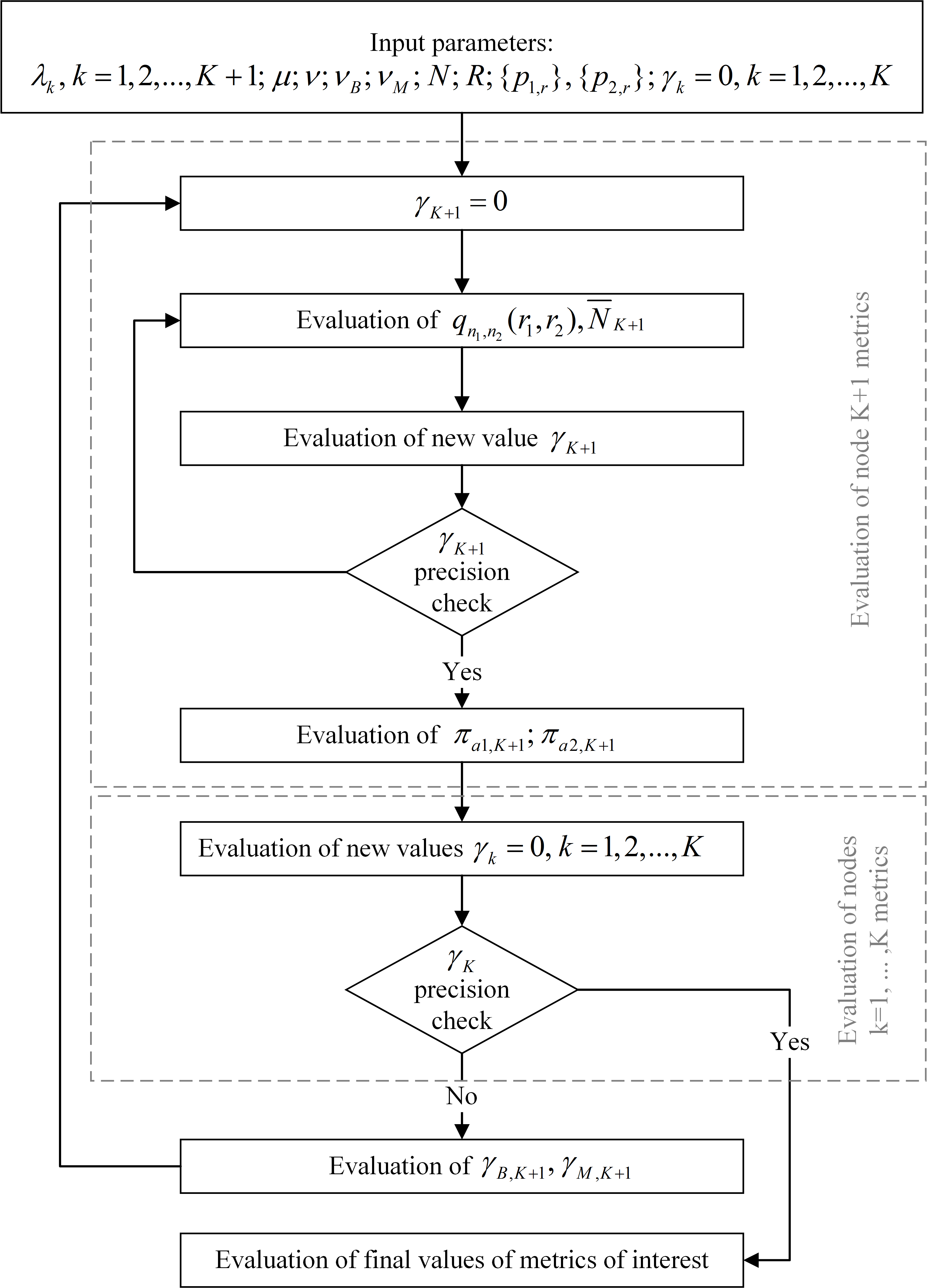
Calculation of (22) requires an iterative algorithm shown in Fig. 10. The algorithm starts with the evaluation of metrics at node with only primary session arrivals (). Stationary distribution , see (15) and (16), and average number of primary and secondary sessions in (17) are calculated. Using the obtained value of , the new value of the secondary sessions arrival intensity is calculated according to (11). If the modulo of the difference between the new and the previous values of is greater than the predefined precision level, the algorithm proceeds to the new iteration. If the desired precision is achieved, the session loss probabilities and are obtained according to (IV-B2). Besides, the new values of are evaluated using (22). Again, if the modulo of the difference between the new and the previous values of is greater than the precision level, the arrival intensities , of the rerouted sessions at node are calculated according to (12), and the algorithm returns to the evaluation of stationary probabilities with new arrival intensities of rerouted sessions and no secondary sessions, i.e. . Otherwise, the stable solution is achieved, and the algorithm proceeds to calculation of final metrics.
References
- [1] M. Shafi, H. Tataria, A. F. Molisch, F. Tufvesson, and G. Tunnicliffe, “Real-Time Deployment Aspects of C-Band and Millimeter-Wave 5G-NR Systems,” arXiv preprint arXiv:2001.11903, 2020.
- [2] M. Giordani, M. Polese, M. Mezzavilla, S. Rangan, and M. Zorzi, “Toward 6G networks: Use cases and technologies,” IEEE Communications Magazine, vol. 58, no. 3, pp. 55–61, 2020.
- [3] B. A. Bilgin, H. Ramezani, and O. B. Akan, “Human blockage model for indoor terahertz band communication,” in 2019 IEEE International Conference on Communications Workshops (ICC Workshops), pp. 1–6, IEEE, 2019.
- [4] J. M. Jornet and I. F. Akyildiz, “Channel modeling and capacity analysis for electromagnetic wireless nanonetworks in the terahertz band,” IEEE Transactions on Wireless Communications, vol. 10, no. 10, pp. 3211–3221, 2011.
- [5] V. Petrov, D. Moltchanov, Y. Koucheryavy, and J. M. Jornet, “Capacity and outage of terahertz communications with user micro-mobility and beam misalignment,” IEEE Transactions on Vehicular Technology, 2020.
- [6] N. Stepanov, , D. Moltchanov, A. Turlikov, and Y. Koucheryavy, “Statistical Analysis and Modeling of User Micromobility for THz Cellular Communications,” IEEE Transactions on Vehicular Technology, 2021.
- [7] R. Vannithamby and S. Talwar, Towards 5G: Applications, requirements and candidate technologies. John Wiley & Sons, 2017.
- [8] 3GPP, “NR; Multi-connectivity; stage 2 (Release 16),” 3GPP TS 37.340 V16.0.0, 3GPP, December 2019.
- [9] M. Polese, M. Giordani, M. Mezzavilla, S. Rangan, and M. Zorzi, “Improved handover through dual connectivity in 5G mmWave mobile networks,” IEEE Journal on Selected Areas in Communications, vol. 35, pp. 2069–2084, Sept. 2017.
- [10] F. B. Tesema, A. Awada, I. Viering, M. Simsek, and G. P. Fettweis, “Mobility modeling and performance evaluation of multi-connectivity in 5G intra-frequency networks,” in IEEE Globecom Workshops (GC Wkshps), pp. 1–6, December 2015.
- [11] M. Gapeyenko, V. Petrov, D. Moltchanov, M. R. Akdeniz, S. Andreev, N. Himayat, and Y. Koucheryavy, “On the degree of multi-connectivity in 5G millimeter-wave cellular urban deployments,” IEEE Transactions on Vehicular Technology, vol. 68, no. 2, pp. 1973–1978, 2019.
- [12] V. Begishev, E. Sopin, D. Moltchanov, R. Kovalchukov, A. Samuylov, S. Andreev, Y. Koucheryavy, and K. Samouylov, “Joint use of guard capacity and multiconnectivity for improved session continuity in millimeter-wave 5G NR systems,” IEEE Transactions on Vehicular Technology, vol. 70, no. 3, pp. 2657–2672, 2021.
- [13] D. Moltchanov, A. Samuylov, E. Lisovskaya, R. Kovalchukov, V. Begishev, E. Sopin, Y. Gaidamaka, and Y. Koucheryavy, “Performance characterization and traffic protection in street multi-band millimeter-wave and microwave deployments,” IEEE Transactions on Wireless Communications, 2021.
- [14] V. Begishev, E. Sopin, D. Moltchanov, R. Pirmagomedov, A. Samuylov, S. Andreev, Y. Koucheryavy, and K. Samouylov, “Performance analysis of multi-band microwave and millimeter-wave operation in 5G NR systems,” IEEE Transactions on Wireless Communications, vol. 20, no. 6, pp. 3475–3490, 2021.
- [15] V. Petrov, M. Komarov, D. Moltchanov, J. M. Jornet, and Y. Koucheryavy, “Interference and SINR in millimeter wave and terahertz communication systems with blocking and directional antennas,” IEEE Transactions on Wireless Communications, vol. 16, no. 3, pp. 1791–1808, 2017.
- [16] J. Kokkoniemi, J. Lehtomäki, and M. Juntti, “Stochastic geometry analysis for mean interference power and outage probability in thz networks,” IEEE Transactions on Wireless Communications, vol. 16, no. 5, pp. 3017–3028, 2017.
- [17] A. Shafie, N. Yang, S. Durrani, X. Zhou, C. Han, and M. Juntti, “Coverage analysis for 3D terahertz communication systems,” IEEE Journal on Selected Areas in Communications, vol. 39, no. 6, pp. 1817–1832, 2021.
- [18] Y. Wu, J. Kokkoniemi, C. Han, and M. Juntti, “Interference and coverage analysis for terahertz networks with indoor blockage effects and line-of-sight access point association,” IEEE Transactions on Wireless Communications, vol. 20, no. 3, pp. 1472–1486, 2020.
- [19] A. Shafie, N. Yang, and C. Han, “Multi-connectivity for indoor terahertz communication with self and dynamic blockage,” in 2020 IEEE International Conference on Communications (ICC), pp. 1–7, IEEE, 2020.
- [20] D. Moltchanov, Y. Gaidamaka, D. Ostrikova, V. Beschastnyi, Y. Koucheryavy, and K. Samouylov, “Ergodic outage and capacity of terahertz systems under micromobility and blockage impairments,” IEEE Transactions on Wireless Communications, 2021.
- [21] W. Wang, J. Wu, N. Li, and R. Song, “Joint user association and resource allocation for mmwave and thz coexistence networks,” in 2021 IEEE Intl Conf on Parallel & Distributed Processing with Applications, Big Data & Cloud Computing, Sustainable Computing & Communications, Social Computing & Networking (ISPA/BDCloud/SocialCom/SustainCom), pp. 1287–1294, IEEE, 2021.
- [22] N. Hassan, M. T. Hossan, and H. Tabassum, “User association in coexisting rf and terahertz networks in 6g,” in 2020 IEEE Canadian Conference on Electrical and Computer Engineering (CCECE), pp. 1–5, IEEE, 2020.
- [23] 3GPP, “NR; Physical channels and modulation (Release 15),” 3GPP TR 38.211, 3GPP, Dec 2017.
- [24] V. Petrov, T. Kurner, and I. Hosako, “Ieee 802.15. 3d: First standardization efforts for sub-terahertz band communications toward 6g,” IEEE Communications Magazine, vol. 58, no. 11, pp. 28–33, 2020.
- [25] P. Nain, D. Towsley, B. Liu, and Z. Liu, “Properties of random direction models,” in IEEE 24th Annual Joint Conference of the IEEE Computer and Communications Societies, vol. 3, pp. 1897–1907, March 2005.
- [26] S. Singh, R. Mudumbai, and U. Madhow, “Interference analysis for highly directional 60-GHz mesh networks: The case for rethinking medium access control,” IEEE/ACM Transactions on Networking, vol. 19, pp. 1513–1527, October 2011.
- [27] A. B. Constantine et al., “Antenna theory: analysis and design,” Microstrip Antennas, John Wiley & Sons, 2005.
- [28] 3GPP, “Study on channel model for frequencies from 0.5 to 100 GHz (Release 14),” 3GPP TR 38.901 V14.1.1, 3GPP, July 2017.
- [29] M. Gapeyenko, A. Samuylov, M. Gerasimenko, D. Moltchanov, S. Singh, E. Aryafar, S.-p. Yeh, N. Himayat, S. Andreev, and Y. Koucheryavy, “Analysis of human-body blockage in urban millimeter-wave cellular communications,” in Communications (ICC), 2016 IEEE International Conference on, pp. 1–7, IEEE, 2016.
- [30] L. S. Rothman et al., “HITRAN: High-resolution transmission molecular absorption database,” tech. rep., Harvard-Smithson Center for Astrophysics, www.cfa.harvard.edu, 2014.
- [31] R. Kovalchukov, D. Moltchanov, A. Samuylov, S. Andreev, Y. Koucheryavy, and K. Samouylov, “Evaluating SIR in 3D millimeter-wave deployments: direct modeling and feasible approximations,” IEEE Transactions on Wireless Communications, vol. 18, no. 2, pp. 879–896, 2019.
- [32] V. Naumov, Y. Gaidamaka, N. Yarkina, and K. Samouylov, Matrix and Analytical Methods for Performance Analysis of Telecommunication Systems. Springer, 2021.
- [33] V. A. Naumov, K. E. Samuilov, and A. K. Samuilov, “On the total amount of resources occupied by serviced customers,” Automation and Remote Control, vol. 77, no. 8, pp. 1419–1427, 2016.
- [34] E. S. Sopin, K. A. Ageev, E. V. Markova, O. G. Vikhrova, and Y. V. Gaidamaka, “Performance analysis of M2M traffic in LTE network using queuing systems with random resource requirements,” Automatic Control and Computer Sciences, vol. 52, no. 5, pp. 345–353, 2018.
- [35] S. Ross, Introduction to probability models. Academic Press, 2010.
- [36] M. Gapeyenko, A. Samuylov, M. Gerasimenko, D. Moltchanov, S. Singh, M. R. Akdeniz, E. Aryafar, N. Himayat, S. Andreev, and Y. Koucheryavy, “On the temporal effects of mobile blockers in urban millimeter-wave cellular scenarios,” IEEE Transactions on Vehicular Technology, available online, 2017.
- [37] J. W. Cohen, The single server queue. Elsevier, 2012.
- [38] Y.-N. R. Li, M. Chen, J. Xu, L. Tian, and K. Huang, “Power saving techniques for 5G and beyond,” IEEE Access, vol. 8, pp. 108675–108690, 2020.