Relativistic Space-Charge Field Calculation by Interpolation-Based Treecode
Abstract
Space-charge effects are of great importance in particle accelerator physics. In the computational modeling, tree-based methods are increasingly used because of their effectiveness in handling non-uniform particle distributions and/or complex geometries. However, they are often formulated using an electrostatic force which is only a good approximation for low energy particle beams. For high energy, i.e., relativistic particle beams, the relativistic interaction kernel may need to be considered and the conventional treecode fails in this scenario. In this work, we formulate a treecode based on Lagrangian interpolation for computing the relativistic space-charge field. Two approaches are introduced to control the interpolation error. In the first approach, a modified admissibility condition is proposed for which the treecode can be used directly in the lab-frame. The second approach is based on the transformation of the particle beam to the rest-frame where the conventional admissibility condition can be used. Numerical simulation results using both methods will be compared and discussed.
Keywords:
Treecode, space-charge field calculation, separable approximation, admissibility condition, special relativity.1 Introduction
Space-charge effects are very important in accelerator physics and can lead to many unwanted phenomena. For example, the space-charge force limits the intensity of the electron current emitted from the cathode inside the electron gun [1] and causes the broadening of ultrafast electron packets in the free-space propagation [2, 3]. In numerical simulations, grid-based methods have been the standard choice. Among all grid-based methods, the particle-in-cell (PIC) method is probably the most popular choice. PIC is a self-consistent model considering the field generation from the charged particle and the field-particle interaction [4]. In the framework of electromagnetic particle-in-cell (EM-PIC), the particle trajectory is used to obtain charge or current density over a spatial grid by a charge deposition scheme [5, 6]. With the charge and current density, the corresponding electromagnetic field is then evaluated by solving Maxwell’s equations [7, 8]. In combination with a suitable numerical integrator [9], the solution of the particle field and a given external field are used to push the particles to their new states of motion. For non-relativistic particle beams, the electrostatic particle-in-cell (ES-PIC) method is usually used where Poisson’s equation is solved to compute the particle field [10]. In addition to the electromagnetic model, the relativistic particle beam can be simulated by a quasi-static model [11, 12] which solves the electrostatic field in the rest-frame of the particle beam and applies the corresponding electromagnetic field in the lab-frame. However, PIC has several numerical issues despite of its popularity. For example, the standard EM-PIC based on the finite-difference time-domain (FDTD) method has numerical dispersion due to the approximation with finite-difference stencils [13]. The pseudo-spectral methods, e.g. the pseudo-spectral time-domain (PSTD) [8] method or the pseudo-spectral analytical time-domain (PSATD) method [14] were used to mitigate this problem by evaluating the spatial derivative in the spectral domain. However, because of the usage of the fast Fourier transform (FFT), the pseudo-spectral method is computationally more demanding compared to FDTD and its performance cannot scale over many computing nodes [15]. Besides, standard PIC uses a fixed size grid to discretize the spatial domain and is inefficient for non-uniform particle distributions [16].
The computation of the space-charge field can also be achieved by a direct -body summation (also called brute-force method). One major advantage of this method is the consideration of coulomb collision effect, which is especially critical in some problems of the accelerator physics [17, 18]. However, a direct -body methods requires a computational cost of and may not be applicable if a large number of particles is considered. Therefore, many efforts have been devoted to the development of tree-based methods where particles are subdivided into a hierarchy of clusters and the hierarchical relation of each cluster is stored in a tree data structure called cluster tree. Treecodes [19] rely on the approximation of particle-cluster interactions and have a complexity down to . The force field on each particle is computed through an independent tree traversal starting from the root cluster and the applicability of the particle-cluster approximation is determined by the multiple acceptance criterion (MAC) which is similar to the admissibility condition in the study of hierarchical (H-) matrices [20, 21]. The fast multipole method (FMM) [22] can further reduce the complexity down to by considering the cluster-cluster interactions. In traditional FMMs, each cluster at the same level is covered by a cubic box of the same size and the cluster-cluster interaction list is determined by a cluster’s neighbor boxes and its parent’s neighbor boxes. Compared to treecodes, one major drawback of traditional FMMs is that the well-separation condition relies on bounding boxes of a fixed size. Such definition of the well-separation condition leads to two problems:
- 1.
Unlike the MAC in treecode, the well-separation condition cannot be flexibly controlled.
- 2.
It excludes the usage of tight bounding boxes (can be of rectangular shape) which have an adaptive size depending on the cluster and are favorable for non-uniform particle distribution.
Therefore, traditional FMMs are inefficient to treat non-uniform particle distributions [23]. There also exist hybrid FMMs merging the strengths from both treecode and traditional FMMs [24, 25, 26]. One effort of hybrid FMMs is based on the dual tree traversal [24, 25] where the cluster-cluster interaction list is determined by traversing the source and target cluster trees simultaneously and the well-separation condition can be defined as flexible as the MAC.
There have been many efforts using tree-based methods to model Coulomb interaction in the study of non-relativistic charged particles, e.g. plasma dynamics [27, 28], electron dynamics in ultrafast electron microscopy [29] and proton dynamics in synchrotrons [30]. For the dynamics of relativistic electron beams, the relativistic interaction kernel needs to be considered as the particles’ field lines get compressed in the transverse direction [31]. The evaluation of the relativistic kernel based on the brute-force method was used in some studies [32, 33] and has been provided in some beam dynamics codes, e.g., the General Particle Tracer (GPT) [34]. To the best of our knowledge, there are few studies on using tree-based methods to calculate the relativistic space-charge field; only some previous works proposed by Schmid et al. can be found [35, 36]. Their approach is based on the quasi-static model: the space-charge field is solved in the particle’s inertial frame by using the FMM with a spherical harmonics expansion [37].
In this study, we first introduce the general concept of a treecode. After that, based on the treecode proposed by Wang et al. [38], we formulate an interpolation-based treecode for computing the relativistic space-charge field. In particular, we propose two methods to control the interpolation error:
- 1.
Based on the analytic estimation of the interpolation error bound, a modified admissibility condition is derived so that the formulated treecode can be performed directly in the lab-frame.
- 2.
The system is first transformed to the rest-frame of the average particle momentum in which the particle field is computed by a treecode and is then transformed back to the lab-frame. By using the relativistic transformation to the rest-frame, the formulated treecode can work with the conventional admissibility condition.
Our numerical results show that the treecode based on the modified admissibility condition has better accuracy than the treecode based on the relativity transformation when a particle beam with momentum spread is considered; an explanation is also provided. Besides, we demonstrate that the proposed treecode scales like .
2 The idea of treecode
In this section, we provide a 2D example to illustrate the idea of treecode. The example provided here can easily be generalized to 3D, all our computations are done in 3D.
In the -body problem, the total force field experienced by a target point can be written as
| (2.1) |
where denotes the index of the source particle with the position in a cluster and denotes the index set of the particles in . Through an interaction kernel , the source particle at applies the force field with the magnitude proportional to a physical quantity of the particle.
When evaluating (2.1), we can divide the source particles contained in into several smaller clusters and split the summation corresponding to
| (2.2) |
where , , and are the sub-clusters located in the relative locations at the left-top, left-bottom, right-top, and right-bottom from the domain of the cluster , respectively (Figure 1(a)). To express things in a general manner, we use to denote the sub-cluster from the -th subdivision (also called level) of the root cluster with the location indices . If the distance from the target point in to , , and is far enough (i.e., fulfills a sort of admissibility condition similar to the far-field condition) and the kernel function can be approximated by a separable expansion with a rank over the domain of a cluster by
| (2.3) |
then the force field from the particles can be approximated by
with
| (2.4) |
Here, is a set of indices for the far-field clusters at each level. In this illustrative example, the target point is in the top-left corner of the domain such that the indices of far-field clusters in each level all belong to the set . In general, depending on the position of the target point, the index of a far-field cluster can be with . The effective physical quantity of the macro particle with the index is denoted by in (2.4). The physical meaning of is that the particles in a cluster are aggregated to a few macro particles; during the evaluation of the force field on the target particle, instead of traversing each real particle in the source cluster, we only consider a few macro particles if the approximation (2.3) is accurate, which is typically the case if the distance to the cluster is large enough.
To evaluate the force field from the source particles inside the cluster , we can apply a similar trick as before. We first subdivide each sub-cluster from the level 1 into four sub-clusters (, , , and ) and then use them to compute the approximated field (Figure 1(b)). Assume that at each level of the subdivision only one cluster does not fulfill the far-field condition. We can compute the force field from , , and by the far-field approximation and subdivide to get the sub-clusters of the next level . This procedure can be applied repeatedly until a maximum level is reached and the approximated force field can be computed by
| (2.5) |
This means that the evaluation of the force-field can be decomposed into near-field and far-field terms. The far-field term is computed approximately by the effective physical quantities of the macro particles inside the far-field clusters of different levels. The near-field term is evaluated directly from the physical quantities of micro particles inside the near-field clusters.
Consider a root cluster containing uniformly distributed particles. If every cluster of the finest level contains particles (i.e., for all ), the number of subdivisions is given by
From a practical point of view it is reasonable to choose so that the number of macro particles in the clusters (2.3) is not less than . Since there are three far-field clusters at each level and one near-field cluster at the finest level, we need to traverse clusters to evaluate the field at . Therefore, the number of terms to evaluate (2.5) becomes
If is bounded and independent of , the computation cost for evaluating the force field experienced by a single particle becomes . This argument can be applied to each particle in the root cluster and the total computation cost for evaluating the interaction force of particles in is .
From the example discussed above, we can see that the success of treecode relies on the hierarchical subdivision of particles into clusters and the approximation of the kernel function through a separable expansion. Thus, in the following sections, the following two main questions will be discussed:
- •
How can we subdivide the particles into a set of hierarchical clusters?
- •
How can we construct a separable approximation of a kernel function and bound the error of this approximation?
3 Cluster tree
A cluster tree [20, 21] is a space-partition data structure (similar to the k-d tree [39]) which provides an efficient way for finding the interaction list in the tree-based method. In this section, we briefly introduce the terminology and the construction of the cluster tree.
Definition 1 (Cluster Tree).
A cluster tree is a labeled tree associated with an index set and fulfills the following requirements:
- •
For the root node , its label set is given by the index set , i.e., .
- •
If is a non-leaf node, its label set is the union of the label sets of its children nodes (i.e., ).
- •
If , then .
We call the label sets associated with nodes of the tree (index) clusters.
Let be given by a set of particle positions (which we also call a cluster of particles) with index set . We denote the entries in a vector by . The tightest rectangular box covering is called the bounding box and is defined as
with , and . To subdivide a cluster containing particles, we first determine which enables us to find the coordinate direction with the biggest interval . We then choose the particle position with the -th greatest value in the -component of its position as the splitting point such that the cluster can be subdivided into two sub-clusters
We can apply this subdivision procedure to each of the resulting sub-clusters repeatedly until the number of particles in the clusters at the deepest level is smaller than a pre-selected number . Different to what has been used in the illustrative example of the previous section, this cardinality-balanced subdivision strategy is used in the remainder of this study since it has the following benefits:
- •
Each subdivided cluster contains roughly the same number of particles so that the cluster tree is balanced regardless of the particle distribution.
- •
The subdivision based on the coordinate direction with the biggest interval can shrink the diameter of the cluster fast.
4 Approximation for the kernel function of the space-charge field
The space-charge field from a relativistic particle at the position experienced by a target position can be expressed as [31, 32]
with
| (4.1) |
Here, and are the Lorentz factor and normalized momentum of the particle, respectively, with the particle velocity normalized to the speed of light. Although not necessary, throughout this study, we assume that each particle in the system has the same charge . In the physics of particle beams moving in the -direction, the paraxial approximation can be usually applied
where , and is the number of particles. Therefore, the kernel function can be approximated as
| (4.2) |
Since , we may use to further simplify equation (4.2) as in (cf. Section A)
| (4.3) |
where . The space-charge field from the source particle can be approximated by
The separable approximation of the kernel function can be achieved by a tensor product interpolation with Lagrangian polynomials [20, 21]
where the Lagrange basis polynomials are defined as
with the interpolation points and the polynomial degree .
The error bound of the tensor product interpolation of the kernel function with respect to the source point variable in a rectangular domain is [21]
| (4.4) |
As indicated by (4.4), to control the interpolation error, we need to find a condition which guarantees a bound for the right-hand-side terms. In the literature, this condition is called admissibility condition [20, 21]. In particular, when determining an admissibility condition for a kernel function , we need to find a bound on the term .
5 Admissibility Condition for the Relativistic Kernel
As mentioned in Section 4, to derive an admissibility condition for a kernel function, it is necessary to bound the higher-order derivatives of the kernel function. For studying the free space electrostatic problem, the force kernel can be written
| (5.1) |
An upper bound of the higher-order derivatives with respect to is given by [21]
and the substitution into (4.4) yields
| (5.2) |
Here, we use the definitions
| (5.3) |
to denote the diameter of and the distance from to .
From (5.2), we can define an admissibility condition (also called -admissibility [21]) for the electrostatic kernel by
with some admissibility parameter .
However, the admissibility condition of the electrostatic kernel (called conventional admissibility condition in this study) may not be used for the relativistic kernel (4.3). Thus, we will derive an upper bound of the interpolation error for the relativistic kernel and derive a corresponding admissibility condition. We first introduce a theorem which is useful for estimating the upper bound of the higher-order derivatives of a specific type of kernel function.
Theorem 1 ([21, Theorem E.4]).
Let with , we have
with a suitable constant . Here, and the following conventions are used [21]:
Since is symmetric with respect to and , the conclusion above also holds for the derivatives with respect to .
The force kernel for the relativistic space-charge field is (4.3)
By introducing a change of variables
the kernel function can be expressed component-wise as
Therefore, the norm of the derivative of along each coordinate direction is
Using Theorem 1 with and , the upper bounds of the norms of the derivatives of are
After the substitution of the upper bounds above into (4.4), the interpolation error becomes
with a three dimensional stretch factor and the set of stretched positions of particle from . Here, the symbol denotes the component-wise product of two vectors. In the derivation above, the equivalence of the two norm and the infinity norm has been used [40].
To express the admissibility condition in the original variables, we define the stretched diameter and the stretched distance
where is a three dimensional stretch factor such that this holds:
Therefore, the stretched admissibility condition for the relativistic kernel can be defined with
| (5.4) |
6 An interpolation-based treecode for evaluating the relativistic space-charge field
When the distance from the particle cluster to the target point fulfills an admissibility condition, the separable approximation to the kernel function through the Lagrangian interpolation can be applied and the space-charge field of the particle cluster can be computed approximately by
| (6.1) | ||||
Here, the quantities
| (6.2) |
are the effective Lorentz factor and the effective momentum of the macro particle with a position in the cluster .
Based on (6.1), we can formulate a treecode for computing the relativistic space-charge field. When the treecode is applied with the stretched admissibility condition, it is advantageous to adjust the procedure to determine the splitting direction. As implied by the stretched diameter in (5.4), the splitting coordinate direction should be determined by the stretched bounding box. Therefore, in the implementation of the treecode with the stretched admissibility condition, a modified strategy to determine the splitting direction is used (Algorithm 6.3 with ).
The formulated treecode (Algorithm 6.1) consists of the two main procedures:
- 1.
A given root particle cluster is subdivided into a hierarchy of smaller clusters (Algorithm 6.2). The splitting direction is determined by the biggest length of the bounding box (Algorithm 6.3 with ) or the stretched bounding box (Algorithm 6.3 with ).
- 2.
In the evaluation of the field on each target point (Algorithm 6.4), an independent traversal of the cluster tree is performed to determine the candidates of the interaction cluster. When a target point to a non-leaf cluster fulfills the conventional admissibility condition (Algorithm 6.5 with ) or the stretched admissibility condition (Algorithm 6.5 with ), the effective quantities are used to compute the space-charge field (6.1). Note that, instead of (5.3), we adapt a different definition to compute the diameter and the distance for the admissibility condition in Algorithm 6.5 because of its simplicity in the practical implementation.
To illustrate the effect of the stretch on the particle-clustering of treecode, we performed 2D simulations for particles uniformly randomly distributed over the unit square . The result is demonstrated in Figure 2.
: stretch factor
: maximum number of particles in the leaf node
: admissibility parameter
: the space-charge field experienced by the -th particle
Function TreecodeStretch
: effective momentum for cluster (global variable) (6.2)
: particle cluster
: stretch factor
: maximum number of particles in the leaf node
Function subdivide
(Algorithm 6.3)
-th largest element of
children(S)
subdivide()
subdivide()
else
: stretch factor
Function direction4split
return end
: effective momentum for cluster (global variable) (6.2)
: position of the target point
: particle cluster
: stretch factor
: admissibility parameter
Function cluster2p
end for
else
end for
: particle cluster
: stretch factor
: admissibility parameter
Function admissible
return end
7 An alternative method based on relativity transformation
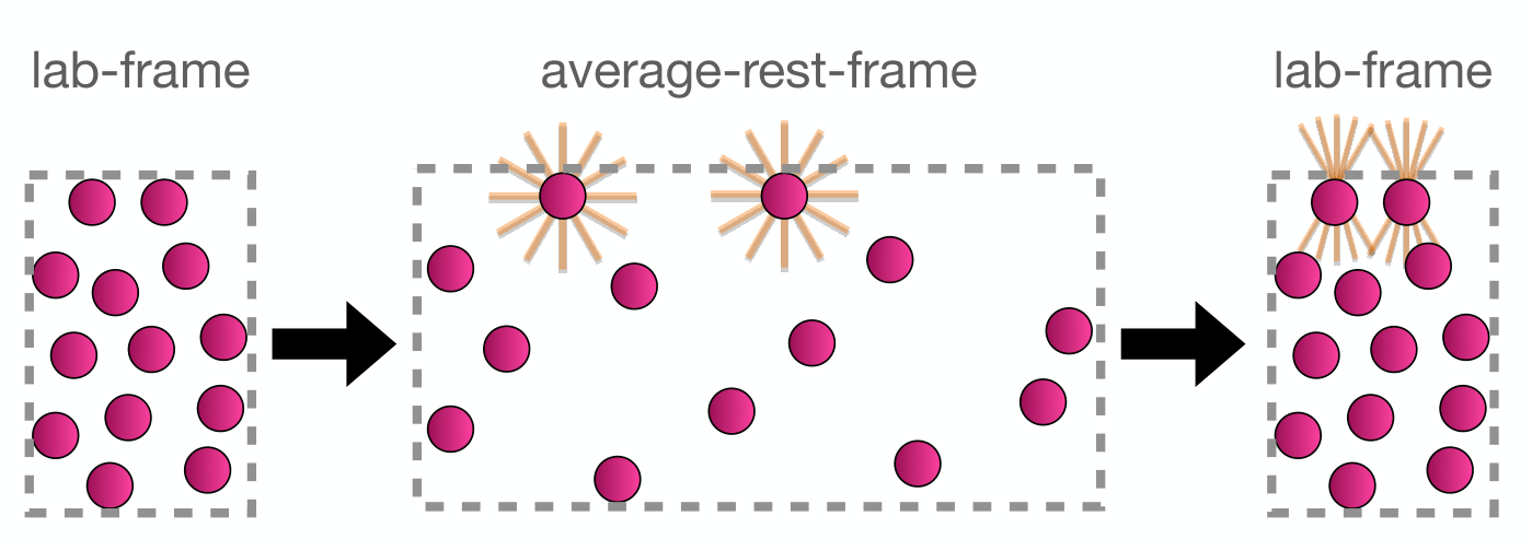
In the previous section we derived an upper bound of the interpolation error for the relativistic interaction kernel and introduced a stretched admissibility condition. In this section we introduce an alternative approach based on the relativity transformation. With this approach, the treecode can be performed without switching to a stretched admissibility condition. We know that the necessity of the stretched admissibility condition comes from the average particle momentum term in the denominator of the relativistic kernel (4.3). If some transformation can be applied to eliminate the average momentum term, we can just use treecode with the conventional admissibility condition. The idea is to transform every physical quantity to the average rest-frame (AVGRF, the inertial frame moving with particle beam’s average momentum) through the Lorentz transformation and evaluate the particle interaction in the frame. In the average rest-frame, the interaction kernel is approximately equal to the electrostatic kernel and treecode can be directly performed with the conventional admissibility condition.
7.1 Particle interaction in the average rest-frame
Let be the average momentum of particles in the system in the lab-frame and be the average rest-frame, in which the average particle momentum is . According to (B.1) and (B.2) with , the position and the momentum in and have the relations
| (7.1) | ||||||
| (7.2) |
where and denote the components parallel and perpendicular to . Here, we use to denote the magnitude of (i.e, ).
The momentum of a particle can be written as and can also be component-wise expressed in the plane spanned by the average momentum and the momentum of the particle as
| (7.3) |
where is the deviation of the particle momentum from with the scalar components , . Throughout this study, we assume that , which is valid in the physics of particle beams.
To eliminate the momentum appearing in the denominator of the relativistic kernel, we can evaluate the particle field in ,
| (7.4) |
where is the vector between source and target particle, and are the Lorentz factor and the momentum of the source particle, respectively. Let denote the deviation to the average Lorentz factor of the particle, . By (7.2) and (7.3), the particle momentum in the average rest-frame can be approximated by
| (7.5) |
where is estimated using the identites and :
Substituting (7.5) into (7.4), the denominator in (7.4) can be approximated by
where the assumption was used. Therefore, the particle field in is approximately equal to
| (7.6) |
After and is computed by the treecode, the corresponding particle field in can be calculated with the field transformation [31]
| (7.7) |
The procedure discussed above is summarized in Algorithm 7.1 and a schematic of the procedure is illustrated in Figure 3. In the practical implementation, instead of (7.1), we use
| (7.8) |
to compute the particle position in the average rest-frame. Because the lab-frame position of particles is given at a common simulation time , both (7.1) and (7.8) lead to the same pair-wise distance between particles at the average-rest frame. Therefore, equations (7.8) can be applied in the computation of particle field by treecode, where only the relative position of particles is of importance.
: stretch factor
: maximum number of particles in the leaf node
: admissibility parameter
: the space-charge field experienced by the -th particle
Function TreecodeAVGRF
Function lab2avgframe
for do
8 Results and discussion
To understand the performance of the different treecodes discussed in this study, we performed numerical simulations for particle beams with different configurations. All the treecodes and algorithms discussed in this study have been implemented as a package NChargedBodyTreecode.jl in the Julia programming language [41]. We refer to the procedure proposed by Wang et al. [38] to compute the effective Lorentz factor and the effective momentum of the macro particle: the Lagrangian polynomials are implemented based on the second form of the barycentric formula [42], and the interpolation points (i.e., the positions of the macro particles) are generated by Chebyshev points of the second kind [38]. .
8.1 Particle beam with single momentum
We first consider particles randomly uniformly distributed in the unit cube where each particle has the same momentum with . The space-charge field (both E- and B-field) experienced by each particle in the system is computed by the following methods:
- 1.
brute-force method where the non-approximated kernel function in (4.1) is used,
- 2.
a treecode called “Treecode-Uniform” using the conventional admissibility condition (Algorithm 6.5 with ),
- 3.
a treecode called “Treecode-Stretch” using the stretched admissibility condition and the subdivision strategy with stretch (Algorithm 6.5 with ),
- 4.
a treecode called “Treecode-AVGRF” using the average rest-frame approach (Algorithm 7.1).
The result from brute-force method serves as a reference to evaluate the speedup and the relative error of different treecodes. The measured error is the maximal relative error in the electrical and magnetic field,
where is the number of particles in the system. The space-charge fields and experienced by the -th particle are computed by treecode and the brute-force method, respectively. The result is shown in Figure 4. As illustrated by Figure 4(a), Treecode-Uniform has large errors and this supports our argument in the beginning that the conventional treecode cannot be used directly for relativistic particle beams. On the other hand, as demonstrated in Figure 4(b) and Figure 4(c), the two proposed treecodes can effectively treat the problem of a relativistic particle beam. Also, we can observe that the errors computed by Treecode-Stretch and Trecode-AVGRF look the same. The reason is that both methods result in equivalent ways to subdivide the particle clusters and to determine the admissible clusters. In Treecode-AVGRF, the particles’ spatial distribution gets boosted along the longitudinal direction after the relativity transformation depicted in Figure 3. In Treecode-Stretch, the particles’ spatial distribution stays unchanged in the lab-frame but the subdivision and the admissibility condition involve a stretch factor related to the Lorentz boost.
8.2 Particle beam with momentum spread
In practical scenarios, beam divergence and energy spread are typically present in particle beams. These two quantities are related to the momentum distribution of a particle beam in transverse and longitudinal direction, respectively. Therefore it is also important to know how the momentum distribution influences the accuracy of treecodes. We consider a particle beam randomly distributed over a momentum distribution defined as
Here, and are equivalent to rms (root mean square) divergence and rms energy spread for a relativistic particle beam with the paraxial approximation (i.e., ). The positions of the particles are uniformly randomly distributed over the unit cube . The result is shown in Figure 5. Our numerical results reveal that treecode-AVGRF is less accurate than Treecode-Stretch when a momentum spread is considered in the particle beam.
8.3 The problem of Treecode-AVGRF
Our numerical results show that Treecode-AVGRF is less accurate compared to Treecode-Stretch when a momentum spread is considered in the particle beam. The reason is due to the inaccurate computation of the target-source distance in the average rest-frame. To explain this, we consider a particle moving with a momentum in the lab-frame (Figure 6(a)). If the positions of the particle and the target point are both measured at the same time , the distance between these two points can be calculated directly using . If we transform the system to a reference frame moving with a momentum (Figure 6(b)), the events observed in will become
Here, we assume with and the space-time quantities are normalized such that the speed of light is . It is problematic if we compute the distance directly by because these two events are measured at different times (i.e., ) and the particle keeps moving during the measurement. To get a correct distance, as demonstrated in Figure 6(c), we need to transform the system to the particle’s rest-frame that satisfies
In the reference frame , although two events are still measured at different times (i.e., ), we can still compute the distance with because the particle is stationary during the measurement. However, this approach is not applicable to treecode because the transformations of the whole particle beam to each particle’s rest-frame have a complexity of .
8.4 Performance
To understand the speedup achieved with our treecode, we compare the performance of the brute-force method and the treecode in Figure 7. Here, Treeecode-Stretch is selected because it has the best accuracy in all the scenarios discussed before. In this performance test, the particles are randomly uniformly distributed in the unit cube and each particle has the same momentum associated with . The elapsed time of treecode represents the execution time of Algorithm 6.1. As shown in Figure 7(a) and Figure 7(c), the brute-force method scales with . The treecode scales between and (Figure 7(a)) and approaches to its theoretical complexity as the number of particles becomes bigger (Figure 7(d)). Also, we can observe that the speedup of the treecode increases with the number of particles (Figure 7(b)). Here, the speedup refers to the ratio of the elapsed time of the brute-force method to the elapsed time of the treecode. Besides, we can observe in Figure 7(e) that the relative error of treecode is independent of .
9 Conclusion
In this study, based on the Lagrangian interpolation, we formulate a treecode for computing the relativistic space-charge field. We propose two approaches to control the interpolation error: Treecode-Stretch and Treecode-AVGRF. Our numerical result shows that Treecode-Stretch has better accuracy than Treecode-AVGRF for particle beams with momentum spread. Also, the performance of our treecode scales like as expected by the theory. Comparing to FMM, which usually relies on a sophisticated data structure, the proposed treecode is easy to implement and intrinsically parallelizable; it may be especially suitable for building in-house solvers for the study of space-charge effects from relativistic beams. For future work, we plan to extend our treecode formulation to FMM and investigate its parallelization under many-cores architectures like graphics processing units (GPU). Some former works, e.g., Ref. [43], might provide a possible direction.
Appendix A Approximation of the denominator of the relativistic kernel function
Lemma 1.
Let be a vector in cylindrical coordinates. If , we have the approximation
Proof.
In cylindrical coordinates, the function can be expressed as
| (A.1) |
To find out the approximation, we analyze the term
| (A.2) |
in three main different cases.
For the cases of and , we first recast (A.2) to
and we can conclude that (A.2) can be approximated by .
Appendix B Some properties of special relativity
This section summaries some consequences of special relativity, which are already discussed in the literature, for example in the textbook of classical electrodynamics [31]. Consider one inertial frame moving with a velocity (corresponding to the momentum ) relative to another frame . The space-time coordinates of an event in these two frames follow the transformation
| (B.1) |
where and denote the components parallel and perpendicular to . Here, we use to denote the magnitude of (i.e, ). Similar to the space-time coordinates, the four-momentum (energy and momentum) in and follows the transformation
| (B.2) |
The transformation formulas for the position and momentum above are expressed in the component-wise form because of its convenience for the theoretical derivation. These transformations can also be expressed in vector form
| (B.3) | ||||
| (B.4) |
Acknowledgement
This work was supported by DASHH (Data Science in Hamburg – HELMHOLTZ Graduate School for the Structure of Matter) with the Grant-No. HIDSS-0002 and in part by the European Research Council under the European Union’s Seventh Framework Programme (FP7/2007-2013) through Synergy Grant (609920). The authors acknowledge the computational resources of the Maxwell Cluster operated at Deutsches Elektronen-Synchrotron (DESY).
References
- [1] J. W. Luginsland, Y. Y. Lau, R. J. Umstattd, J. J. Watrous, Beyond the Child–Langmuir law: A review of recent results on multidimensional space-charge-limited flow, Physics of Plasmas 9 (5) (2002) 2371–2376. doi:10.1063/1.1459453.
- [2] B. J. Siwick, J. R. Dwyer, R. E. Jordan, R. J. D. Miller, Ultrafast electron optics: Propagation dynamics of femtosecond electron packets, Journal of Applied Physics 92 (3) (2002) 1643–1648. doi:10.1063/1.1487437.
- [3] S. Collin, M. Merano, M. Gatri, S. Sonderegger, P. Renucci, J.-D. Ganière, B. Deveaud, Transverse and longitudinal space-charge-induced broadenings of ultrafast electron packets, Journal of Applied Physics 98 (9) (2005) 094910. doi:10.1063/1.2128494.
- [4] J. M. Dawson, Particle simulation of plasmas, Rev. Mod. Phys. 55 (1983) 403–447. doi:10.1103/RevModPhys.55.403.
- [5] T. Esirkepov, Exact charge conservation scheme for Particle-in-Cell simulation with an arbitrary form-factor, Computer Physics Communications 135 (2) (2001) 144–153. doi:10.1016/S0010-4655(00)00228-9.
- [6] T. Umeda, Y. Omura, T. Tominaga, H. Matsumoto, A new charge conservation method in electromagnetic particle-in-cell simulations, Computer Physics Communications 156 (1) (2003) 73–85. doi:10.1016/S0010-4655(03)00437-5.
- [7] K. Yee, Numerical solution of initial boundary value problems involving Maxwell’s equations in isotropic media, IEEE Transactions on Antennas and Propagation 14 (3) (1966) 302–307. doi:10.1109/TAP.1966.1138693.
- [8] Q. H. Liu, The pseudospectral time-domain (PSTD) method: a new algorithm for solutions of Maxwell’s equations, in: IEEE Antennas and Propagation Society International Symposium 1997. Digest, Vol. 1, 1997, pp. 122–125. doi:10.1109/APS.1997.630102.
- [9] J. P. Boris, Relativistic plasma simulation-optimization of a hybrid code, in: Proc. Fourth Conf. Num. Sim. Plasmas, Naval Res. Lab, Wash. DC, 1970, pp. 3–67.
- [10] C. K. Birdsall, A. B. Langdon, Plasma physics via computer simulation, CRC press, 2018.
- [11] K. Flöttmann, S. Lidia, P. Piot, Recent improvements to the ASTRA particle tracking code, Tech. rep., Lawrence Berkeley National Lab (LBNL), Berkeley, CA (United States) (2003).
- [12] J. Qiang, Symplectic multiparticle tracking model for self-consistent space-charge simulation, Phys. Rev. Accel. Beams 20 (2017) 014203. doi:10.1103/PhysRevAccelBeams.20.014203.
- [13] A. Taflove, S. C. Hagness, M. Piket-May, Computational electromagnetics: the finite-difference time-domain method, The Electrical Engineering Handbook 3 (2005).
- [14] I. Haber, R. Lee, H. Klein, J. Boris, Advances in electromagnetic simulation techniques, in: Proc. Sixth Conf. Num. Sim. Plasmas, Berkeley, CA, 1973, pp. 46–48.
- [15] R. Lehé, J.-L. Vay, Review of spectral Maxwell solvers for electromagnetic particle-in-cell: Algorithms and advantages, in: Proceedings of the 13th International Computational Accelerator Physics Conference, Key West, FL, USA, 2018, pp. 20–24.
- [16] H. Zhang, H. Huang, R. Li, J. Chen, L.-S. Luo, Fast multipole method using Cartesian tensor in beam dynamic simulation, AIP Conference Proceedings 1812 (1) (2017) 050001.
- [17] M. Reiser, Theory and design of charged particle beams, John Wiley & Sons, 2008.
- [18] M. Gordon, S. Van Der Geer, J. Maxson, Y.-K. Kim, Point-to-point coulomb effects in high brightness photoelectron beam lines for ultrafast electron diffraction, Physical Review Accelerators and Beams 24 (8) (2021) 084202. doi:10.1103/PhysRevAccelBeams.24.084202.
- [19] J. Barnes, P. Hut, A hierarchical O(N log N) force-calculation algorithm, Nature 324 (6096) (1986) 446–449.
- [20] S. Börm, Efficient numerical methods for non-local operators: -matrix compression, algorithms and analysis, Vol. 14 of EMS Tracts in Mathematics, European Mathematical Society (EMS), Zürich, 2010. doi:10.4171/091.
- [21] W. Hackbusch, Hierarchical matrices: algorithms and analysis, Vol. 49, Springer, 2015.
- [22] L. Greengard, V. Rokhlin, A fast algorithm for particle simulations, Journal of Computational Physics 73 (2) (1987) 325–348.
- [23] R. Capuzzo-Dolcetta, P. Miocchi, A comparison between the fast multipole algorithm and the tree-code to evaluate gravitational forces in 3-D, Journal of Computational Physics 143 (1) (1998) 29–48.
- [24] M. S. Warren, J. K. Salmon, A portable parallel particle program, Computer Physics Communications 87 (1-2) (1995) 266–290.
- [25] W. Dehnen, A hierarchical O(N) force calculation algorithm, Journal of Computational Physics 179 (1) (2002) 27–42.
- [26] H. Cheng, L. Greengard, V. Rokhlin, A fast adaptive multipole algorithm in three dimensions, Journal of Computational Physics 155 (2) (1999) 468–498.
- [27] S. Pfalzner, P. Gibbon, A 3D hierarchical tree code for dense plasma simulation, Computer physics communications 79 (1) (1994) 24–38.
- [28] D. Thomas, J. Holgate, A treecode to simulate dust–plasma interactions, Plasma Physics and Controlled Fusion 59 (2) (2016) 025002.
- [29] H. Zhang, J. Portman, Z. Tao, P. Duxbury, C.-Y. Ruan, K. Makino, M. Berz, The differential algebra based multiple level fast multipole algorithm for 3D space charge field calculation and photoemission simulation, Microscopy and Microanalysis 21 (S4) (2015) 224–229.
- [30] F. W. Jones, A hybrid fast-multipole technique for space-charge tracking with halos, AIP Conference Proceedings 448 (1) (1998) 359–370. doi:10.1063/1.56759.
- [31]
J. D. Jackson, Classical
electrodynamics, 3rd Edition, Wiley, New York, NY, 1999.
URL http://cdsweb.cern.ch/record/490457 - [32] A. Sell, F. X. Kärtner, Attosecond electron bunches accelerated and compressed by radially polarized laser pulses and soft-x-ray pulses from optical undulators, Journal of Physics B: Atomic, Molecular and Optical Physics 47 (1) (2013) 015601.
- [33] I. V. Kochikov, R. J. Dwayne Miller, A. A. Ischenko, Relativistic modeling of ultra-short electron pulse propagation, Journal of Experimental and Theoretical Physics 128 (3) (2019) 333–340.
- [34] S. Van der Geer, M. De Loos, D. Bongerd, General particle tracer: A 3D code for accelerator and beam line design, in: Proc. 5th European Particle Accelerator Conf., Stockholm, 1996.
- [35] S. A. Schmid, H. D. Gersem, E. Gjonaj, REPTIL - A Relativistic 3D Space Charge Particle Tracking Code Based on the Fast Multipole Method, presented at ICAP2018 in Key West, FL, USA, unpublished (Jan. 2019).
- [36] S. Schmid, H. De Gersem, M. Dohlus, E. Gjonaj, Simulating Space Charge Dominated Beam Dynamics Using FMM, in: 3rd North American Particle Accelerator Conference (NAPAC2019), 2019, p. WEPLE10. doi:10.18429/JACoW-NAPAC2019-WEPLE10.
- [37] J. Kurzak, B. M. Pettitt, Fast multipole methods for particle dynamics, Molecular simulation 32 (10-11) (2006) 775–790.
- [38] L. Wang, R. Krasny, S. Tlupova, A kernel-independent treecode based on barycentric Lagrange interpolation, Communications in Computational Physics 28 (4) (2020) 1415–1436.
- [39] J. L. Bentley, Multidimensional binary search trees used for associative searching, Communications of the ACM 18 (9) (1975) 509–517.
- [40] K. Conrad, Equivalence of norms, Expository Paper, University Of Connecticut, Storrs 17 (2018) 2018.
- [41] J. Bezanson, A. Edelman, S. Karpinski, V. B. Shah, Julia: A fresh approach to numerical computing, SIAM Review 59 (1) (2017) 65–98. doi:10.1137/141000671.
- [42] J.-P. Berrut, L. N. Trefethen, Barycentric Lagrange interpolation, SIAM Review 46 (3) (2004) 501–517.
- [43] L. Wilson, N. Vaughn, R. Krasny, A gpu-accelerated fast multipole method based on barycentric lagrange interpolation and dual tree traversal, Computer Physics Communications 265 (2021) 108017. doi:https://doi.org/10.1016/j.cpc.2021.108017.