Observability of lensing of gravitational waves
from massive black hole binaries with LISA

Let us first consider the simple case of a PM lens, for which the mass density $\rho_{\mathrm{PM}}(\bm{r})=M_{\mathrm{L}}\delta^{3}(\bm{r})$. Here, $\delta^{3}(\bm{r})$ is the three-dimensional Dirac delta function. A natural choice for $\xi_{0}$ is the Einstein radius, i.e.,

With this choice, we have $\psi(x)=\ln x$, and the radial integral can be solved analytically with the result Takahashi and Nakamura 2003

Here, $w=8\pi M_{\rm L}(1+z_{\rm L})f$, $\phi(y)=(x_{+}-y)^{2}/2-\ln x_{+}$, $x_{+}=[(y^{2}+4)^{1/2}+y]/2$, and ${{}_{1}F_{1}}(a,b;z)$ is the confluent hypergeometric function.

For a singular isothermal sphere with velocity dispersion $\sigma_{v}$, the mass density reads $\rho_{\mathrm{SIS}}(\bm{r})=\sigma_{v}^{2}/(2\pi|\bm{r}|^{2})$. For an axially-symmetric gravitational lens, the lens mass $M_{\rm L}$ is defined as the amount of mass enclosed within the Einstein radius of the lens. Therefore, the total mass of the lens and the lens mass are equivalent for a point-mass lens. This may not be the case for other lens profiles; for example, the total mass of a dark matter halo with the SIS profile is different from the lens mass of the halo. For the SIS profile, the lens mass is related to $\sigma_{v}$ as

The Einstein radius is

and $w=8\pi M_{\rm L}(1+z_{\rm L})f$ (as in the case of a PM lens).

We choose the normalization to be $\xi_{0}$, giving $\psi(x)=x$ and $\phi(y)=y+1/2$ in Eq. (5) for the SIS lens. The resulting formula for the radial integral can be found in Ref. Takahashi and Nakamura 2003. The numerical evaluation of this formula is difficult for large values of $w$ and $y$ since both the exponential and Bessel-function factors in the integrand can oscillate rapidly.

Several different numerical approaches have been proposed to tackle this problem Ulmer and Goodman 1995; Nakamura and Deguchi 1999; Takahashi and Nakamura 2003. Here, we propose and implement a simple, effective method based on a Taylor expansion²² 2 After our pre-print appeared on the arXiv, Ryuichi Takahashi brought to our attention that a perturbative expansion of the lensing potential to find analytical solution of the diffraction integral for SIS lenses was also proposed in Ref. Matsunaga and Yamamoto 2006. of the exponential factor $\exp[-iw\psi(x)]$ in Eq. (5). We begin our evaluation by defining the integral³³ 3 This integral corresponds to Eq. (6.631.1) in Ref. Gradshteyn and Ryzhik 2007 if we make the substitutions $\alpha=-iw/2$, $\beta=wy$, $\mu=n+1$, and $\nu=0$.

where $N\equiv(n+2)/2$. We also define the series expansion of the exponential of the potential,

Using these definitions, Eq. (5) can then be evaluated by integrating the expansion term by term, which gives

This series is usually only conditionally convergent or even divergent, but it can be summed with the help of series acceleration techniques. For an SIS lens, $\psi(x)=x$, so $\Psi_{n}(w)=(-iw)^{n}/n!$, and the Shanks transformation (e.g., see Press et al. 1992) performs well in accelerating the summation. When $(w,y)$ approaches the geometric-optics limit, this series requires very-high floating-point precision and sufficiently many terms to provide satisfactory convergence. So, in practice, we use a piecewise strategy to evaluate $F(w,y)$ with the help of geometric-optics approximation, detailed in Appendix A.

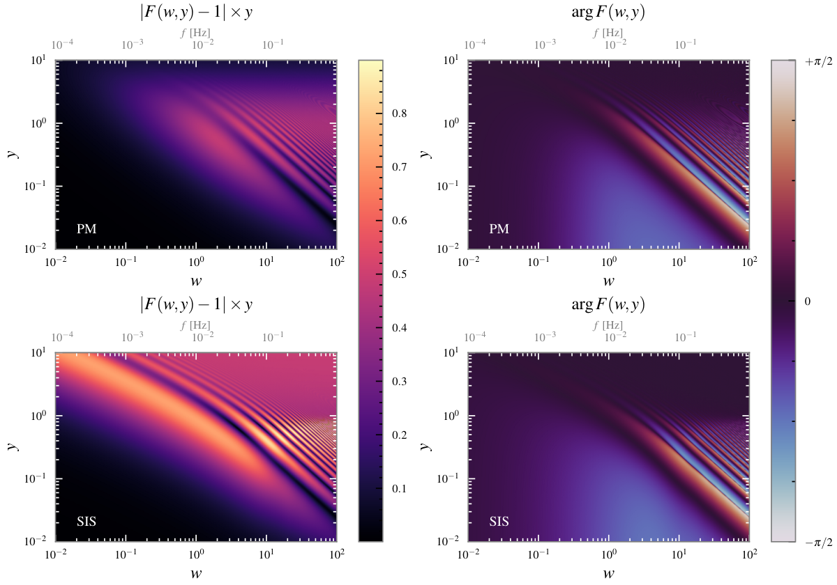
Diffraction integrals computed using Eq. (8) (for PM lenses, top panels) and this analytical solution (for SIS lenses, bottom panels) are shown in Fig. 1. For a given impact parameter $y$, at sufficiently small values of the dimensionless frequency $w$, the lensing effect is negligible because the lens size is negligible compared to the wavelength of GWs. As $w$ increases, the effect of lensing starts to be visible through the oscillations of $F(w,y)$ as a function of $w$. The value of $w$ marking the transition between these two regimes depends on the impact parameter $y$.

In closing this section, let us note that the total mass of the SIS profile is, strictly speaking, infinite. This nonphysical behavior is conventionally regularized by introducing an outer boundary at $r=r_{\Delta}$ such that $\rho_{\mathrm{SIS}}(r_{\Delta})=\Delta\rho_{\mathrm{cr}}$, where $\Delta$ is a dimensionless constant (we set $\Delta=200$), and $\rho_{\mathrm{cr}}=3H_{\mathrm{L}}^{2}/(8\pi)$ is the critical density of the Universe at the redshift $z_{\mathrm{L}}$ with the corresponding Hubble parameter $H_{\mathrm{L}}$. In Appendix B, we demonstrate that this truncation does not affect our results.

Our goal is to improve over the pioneering TN analysis Takahashi and Nakamura 2003 by considering the effects of the merger, ringdown, and higher harmonics. In their work, the errors in the lens mass and impact parameter were estimated for a single MBHB and scaled by the source SNR to estimate the measurement uncertainty of lens parameters for other lensed MBHBs. More importantly, the TN analysis predated the 2005 numerical relativity breakthrough and therefore neither included the merger and ringdown nor higher harmonics. Furthermore, their work does not include an exploration of how other source parameters (such as the binary’s inclination angle and component spins) affect the measurement of the lens parameters.

We estimate measurement uncertainties on $M_{\rm Lz}$ and $y$ for $\mathcal{O}(100)$ MBHBs with fixed intrinsic parameters (to begin with, we fix the detector-frame total mass $M_{\rm Tz}=2\times 10^{6}\,M_{\odot}$, mass ratio $q=1$, and redshift $z_{\rm S}=1$), and randomly sampled extrinsic parameters (inclination angle $\iota$, coalescence phase $\phi_{c}$, right ascension $\lambda$, declination $\beta$, and polarization angle $\psi$) over uniform distributions. To understand the effect of the merger/ringdown, higher-order modes, and spins, we focus on four representative waveform models: (i) a nonspinning IMRPhenomD model where the signal is truncated at the innermost stable circular orbit (henceforth ISCO), which includes only the inspiral part of the waveform and closely mimics the TN results; (ii) a nonspinning IMRPhenomD model including the merger and ringdown (MR); (iii) a nonspinning IMRPhenomHM model including both MR and higher-order modes (HM); (iv) an IMRPhenomHM model with extremal spins aligned with the orbital angular momentum ($\chi_{1}=\chi_{2}=1$), henceforth IMRPhenomHM+; and (v) an IMRPhenomHM model with extremal spins anti-aligned with respect to the orbital angular momentum ($\chi_{1}=\chi_{2}=-1$), henceforth IMRPhenomHM-.

Figure 3 shows how well the observation of a “typical” MBHB by LISA could constrain the mass of a PM lens in the redshifted-lens-mass range $M_{\rm Lz}\in[10^{3},10^{9}]\,M_{\odot}$. For concreteness, we focus on a single value of the impact parameter $y=0.1$. We consider the five waveform models listed above, and we do not normalize the results by the SNR. The general trend with mass is similar to the findings of the inspiral-only TN analysis (see the left panel of Fig. 7 in Takahashi and Nakamura 2003), but our calculations allow us to quantify the effect of the merger/ringdown, higher harmonics, and spins. By comparing nonspinning binaries with the signal truncated at the ISCO with those including merger and ringdown (MR), we see that the inclusion of merger and ringdown leads to improvements by about one order of magnitude in the measurement of the lens mass. Models with higher harmonics (IMRPhenomHM, in green) lead to further improvements in measurement accuracy relative to models without higher harmonics (IMRPhenomD, in red), as expected. The dependence of the waveform on the angles is more pronounced when we include higher harmonics. As a consequence, the measurement errors for IMRPhenomHM have a larger “spread” around the median compared to the measurement errors for IMRPhenomD. It is also well known that aligned (anti-aligned) spins typically increase (reduce) the SNR because of the orbital hang-up effect Campanelli et al. 2006, and indeed we find that measurement errors are smallest for extremal aligned spins (IMRPhenomHM+, in brown) and largest for extremal anti-aligned spins (IMRPhenomHM-, in blue). For lens masses $M_{\rm Lz}\gtrsim 10^{7}\,M_{\odot}$, the geometric-optics limit is a good approximation, and $\Delta M_{\rm Lz}/M_{\rm Lz}$ depends solely on the SNR and the impact parameter $y$ Takahashi and Nakamura 2003. Since in this calculation we have fixed $y$, the uncertainties in the large-$M_{\rm Lz}$ regime shown in Fig. 3 are inversely proportional to the SNR of the signal.

Given the intrinsic parameters of an MBHB, we are interested in estimating the “critical lens mass” $M_{\rm Lz}^{\rm crit}$, defined as the lowest lens mass for which we can extract information on either $M_{\rm Lz}$ or $y$. We (somewhat arbitrarily) define this threshold as the lens mass corresponding to a 100% relative uncertainty on the respective parameter. For the MBHB considered in Fig. 3, we find $M_{\rm Lz}^{\rm crit}=1.08\begin{subarray}{c}+0.64\\ -0.40\end{subarray}\times 10^{5}\,M_{\odot}$ for IMRPhenomD truncated at the ISCO, $M_{\rm Lz}^{\rm crit}=4.73\begin{subarray}{c}+2.45\\ -1.75\end{subarray}\times 10^{3}\,M_{\odot}$ for IMRPhenomD, $M_{\rm Lz}^{\rm crit}=3.19\begin{subarray}{c}+1.39\\ -1.17\end{subarray}\times 10^{3}\,M_{\odot}$ for IMRPhenomHM, $M_{\rm Lz}^{\rm crit}=1.49\begin{subarray}{c}+0.62\\ -0.49\end{subarray}\times 10^{3}\,M_{\odot}$ for IMRPhenomHM+, and $M_{\rm Lz}^{\rm crit}=6.63\begin{subarray}{c}+3.46\\ -2.24\end{subarray}\times 10^{3}\,M_{\odot}$ for IMRPhenomHM-. The quoted values correspond to the median and $68\%$ confidence interval of each critical lens mass. We find that the critical lens mass decreases when we include the merger and higher harmonics in the waveform model, as well as for MBHBs with large aligned spins, in agreement with the trends described earlier.

We can estimate in a similar way the critical impact parameter $y^{\rm crit}$ below which we can extract information on at least one of the lens parameters. We consider the same MBHB, but we now assume a PM lens with fixed redshifted mass $M_{\rm Lz}=10^{7}\,M_{\odot}$, and we vary the impact parameter in the range $y\in[0.01,200]$. The relative uncertainty in $y$ follows the same qualitative trends as the uncertainties in $M_{\rm Lz}$ as we vary the waveform model, and the critical impact parameters are $y^{\rm crit}=52.6\begin{subarray}{c}+17.4\\ -10.1\end{subarray}$ for IMRPhenomD truncated at the ISCO, $y^{\rm crit}=92.4\begin{subarray}{c}+24.5\\ -16.6\end{subarray}$ for IMRPhenomD, $y^{\rm crit}=92.0\begin{subarray}{c}+36.5\\ -17.3\end{subarray}$ for IMRPhenomHM, $y^{\rm crit}=114\begin{subarray}{c}+39\\ -25\end{subarray}$ for IMRPhenomHM+, and $y^{\rm crit}=86.8\begin{subarray}{c}+21.1\\ -19.4\end{subarray}$ for IMRPhenomHM-.

In summary: the inspiral-only waveforms used in TN lead, in general, to an overestimate of measurement uncertainties in the lens parameters relative to waveforms including also the merger and ringdown. For this reason, their results should be regarded as conservative. The merger, ringdown, and higher-order modes can significantly improve our ability to measure the lens mass, and the “critical” measurable lens mass $M_{\rm Lz}^{\rm crit}$ varies by a factor of $\sim 2$ or $3$ for MBHBs with large (anti)aligned spins.

We now focus on the effect of the source parameters on the measurement of $M_{\rm Lz}$ and $y$. We consider IMRPhenomHM MBHB waveforms with $M_{\rm Tz}=10^{7}\,M_{\odot}$, $q=1.2$, $z_{\rm S}=5$, and five selected values of the aligned binary component spins: $\chi_{1}=\chi_{2}\in\{-1,-0.5,0,0.5,1\}$. To begin with, we focus on PM lenses with $y=0.1$ and $M_{\rm Lz}\in[10^{3},10^{9}]\,M_{\odot}$.

We examine the effect of various parameters, namely: the inclination angle $\iota$; the magnitude of the spins; and, finally, the sky location angles (right ascension $\lambda$ and declination $\beta$), mass ratio $q$, coalescence phase $\phi_{c}$, and polarization angle $\psi$. We consider $\mathcal{O}(100)$ random values for each set of parameters that we vary and fix all angles that are not being varied to an “intermediate” value of $\pi/3$.

When we explore the effect of each source parameter, we either normalize the resulting errors in the lens parameters to a reference $\textrm{SNR}=1000$, or we consider MBHBs at fixed redshift. This allows us to understand whether the lens parameter estimation accuracy is dominated by the SNR of the source or by more subtle features related to the specific parameter we vary. For example, higher harmonics (when detectable) can reduce correlations between parameters, and the relative importance of higher harmonics is strongly affected by the inclination of the binary. We will now describe our findings for each parameter.

So far, we have investigated how the measurement of lens parameters is affected by waveform modeling and source parameters. We will now consider three representative MBHBs and compute lens parameter estimation accuracy for a wide range of lens masses and impact parameters. In this section, we focus on PM lenses with $y\in[0.01,200]$ and $M_{\rm Lz}\in[10^{3},10^{9}]\,M_{\odot}$.

In Fig. 7, we show contour plots of $\Delta M_{\rm Lz}/M_{\rm Lz}$ (left panels) and $\Delta y/y$ (right panels) in the $(M_{\rm Lz},\,y)$ plane. Different rows refer to three different nonspinning MBHBs with detector-frame mass $M_{\rm Tz}=10^{8}\,M_{\odot}$, $q=1.2$, $z_{\rm S}=1$ (top); $M_{\rm Tz}=10^{7}\,M_{\odot}$, $q=1.2$, $z_{\rm S}=5$ (middle); and $M_{\rm Tz}=10^{6}\,M_{\odot}$, $q=1.2$, $z_{\rm S}=8$ (bottom). These masses and redshifts have been chosen as representative of typical MBHB systems observable by LISA (see, e.g., Sesana et al. 2011; Klein et al. 2016; Toubiana et al. 2021). To reduce computational time, the angles $\iota$, $\phi_{c}$, $\lambda$, $\beta$ and $\psi$ were all set to $\pi/3$. The range of variability of the results around these “intermediate” values was discussed in Sec. IV.2 above.

The SNRs of the unlensed signals from these MBHBs are $697,\,716,$ and $182$ for the top, middle, and bottom panels in Fig. 7, respectively. When the signals are lensed, the SNRs increase up to $\sim 5970$, $\sim 9180$, and $\sim 2050$ for the top, middle, and bottom panels, respectively.

Three white contour lines in each panel highlight the 100%, 10%, and 1% relative uncertainty boundary regions. In the black regions (outside the outermost white contour), the relative uncertainty is greater than 100%, and therefore at least one of the lensing parameters is unmeasurable. In fact, in some regions of the parameter space, we can measure only one of the lens parameters.

Consider, for example, an MBHB with $M_{\rm Tz}=10^{8}\,M_{\odot}$ at $z_{\rm S}=1$ (top row) with lens parameters $M_{\rm Lz}\approx 10^{7}\,M_{\odot}$ and $y\approx 0.1$: in this case the lens mass can be measured with $\approx 10\%$ relative uncertainty, but $y$ is unmeasurable. For this same binary, $M_{\rm Lz}$ is measurable when $y\lesssim 30$ and $M_{\rm Lz}\gtrsim 10^{6}\,M_{\odot}$ (top left panel), while $y$ is measurable when $y\lesssim 40$ (top right panel). These “detectability boundaries” are slightly different for lighter binaries. We show representative examples in Table 1. Based on this extensive analysis, we conclude that the critical values of $y^{\rm crit}$ and $M_{\rm Lz}^{\rm crit}$ are more optimistic than the TN predictions for PM lenses because the merger/ringdown and higher-order modes sensibly reduce the errors in the lens parameters.

We now consider the same MBHBs as in Sec. IV.3, but we extend the analysis to SIS lenses with $y\in[0.01,200]$ and $M_{\rm Lz}\in[10^{1},10^{8}]\,M_{\odot}$. In Fig. 8, we show contour plots of $\Delta M_{\rm Lz}/M_{\rm Lz}$ (left panels) and $\Delta y/y$ (right panels) in the $(M_{\rm Lz},y)$ plane. Once again, we set all angles ($\iota$, $\phi_{c}$, $\lambda$, $\beta$, $\psi$) equal to $\pi/3$.

The SNRs of the unlensed signals were listed in Sec. IV.3. When the signals are lensed, the SNRs increase up to $\sim 2620$, $\sim 7660$, and $\sim 1180$ for the top, middle, and bottom MBHBs in Fig. 8.

For the binary with $M_{\rm Tz}=10^{8}\,M_{\odot}$ (top row), $M_{\rm Lz}$ is measurable when $y\lesssim 20$ and $M_{\rm Lz}\gtrsim 6\times 10^{5}\,M_{\odot}$, while $y$ is measurable when $y\lesssim 45$. In some regions of the parameter space, we can measure only one of the lens parameters. A qualitative difference with respect to PM lenses is that $y^{\rm crit}$ is no longer (approximately) constant, but it depends on $M_{\rm Lz}$ (as expected from, e.g., Fig. 10 of TN). We summarize the results for each binary in Table 2.

For the binary with $M_{\rm Tz}=10^{7}\,M_{\odot}$ (middle row), we find that the highest $y^{\rm crit}$ corresponds to $M_{\rm Lz}\approx 10^{4}\,M_{\odot}$. Ref. Gao et al. 2022 found the maximum value of the inner product defining the Lindblom criterion, $\langle\delta h|\delta h\rangle\approx 6$, occurs for a comparable value of $M_{\rm Lz}$, and that $\langle\delta h|\delta h\rangle$ decreases – while still satisfying the condition $\langle\delta h|\delta h\rangle>1$ – for lower values of $M_{\rm Lz}$. Note, however, that, according to our analysis, none of the lens parameters is measurable for $M_{\rm Lz}\lesssim 3\times 10^{3}\,M_{\odot}$. This implies that the Lindblom criterion is necessary but not sufficient to conclude whether lensing is observable.

Our findings are significantly more optimistic than those in TN: by including the merger, ringdown, and higher harmonics, we can measure lens parameters for higher values of $y$ and lower values of $M_{\rm Lz}$ than previously thought. Even if we consider a more stringent measurability criterion (setting the threshold at, say, 10% relative uncertainty), we still find that we can extract information about the lens parameters for higher values of $y$ and lower values of $M_{\rm Lz}$ than estimated by TN. As in the case of PM lenses, the values of $M_{\rm Lz}^{\rm crit}$ and $y^{\rm crit}$ have a strong dependence on the parameters of the source and the lens. The simple estimates of lensing probability by TN assumed $y^{\rm crit}$ to be constant, but a more careful estimate should consider the dependence of $M_{\rm Lz}^{\rm crit}$ or $y^{\rm crit}$ on the source and lens parameters.

References

- Bartelmann (2010) M. Bartelmann, Class. Quant. Grav. 27, 233001 (2010), arXiv:1010.3829 [astro-ph.CO] .
- Clowe et al. (2004) D. Clowe, A. Gonzalez, and M. Markevitch, Astrophys. J. 604, 596 (2004), arXiv:astro-ph/0312273 .
- Markevitch et al. (2004) M. Markevitch, A. Gonzalez, D. Clowe, A. Vikhlinin, L. David, W. Forman, C. Jones, S. Murray, and W. Tucker, Astrophys. J. 606, 819 (2004), arXiv:astro-ph/0309303 .
- Bond et al. (2004) I. A. Bond et al., Astrophys. J. Lett. 606, L155 (2004), arXiv:astro-ph/0404309 .
- Treu and Marshall (2016) T. Treu and P. J. Marshall, A&A Rev. 24, 11 (2016), arXiv:1605.05333 [astro-ph.CO] .
- Coe et al. (2013) D. Coe et al., Astrophys. J. 762, 32 (2013), arXiv:1211.3663 [astro-ph.CO] .
- Ohanian (1974) H. Ohanian, Int. J. Theor. Phys. 9, 425 (1974).
- Thorne (1982) K. Thorne, in Les Houches Summer School on Gravitational Radiation (1982) pp. 1–57.
- Deguchi and Watson (1986) S. Deguchi and W. D. Watson, Phys. Rev. D 34, 1708 (1986).
- Wang et al. (1996) Y. Wang, A. Stebbins, and E. L. Turner, Phys. Rev. Lett. 77, 2875 (1996), arXiv:astro-ph/9605140 .
- Nakamura (1998) T. T. Nakamura, Phys. Rev. Lett. 80, 1138 (1998).
- Takahashi and Nakamura (2003) R. Takahashi and T. Nakamura, Astrophys. J. 595, 1039 (2003), arXiv:astro-ph/0305055 .
- Hannuksela et al. (2020) O. A. Hannuksela, T. E. Collett, M. Çalışkan, and T. G. F. Li, Mon. Not. Roy. Astron. Soc. 498, 3395 (2020), arXiv:2004.13811 [astro-ph.HE] .
- Sereno et al. (2011) M. Sereno, P. Jetzer, A. Sesana, and M. Volonteri, Mon. Not. Roy. Astron. Soc. 415, 2773 (2011), arXiv:1104.1977 [astro-ph.CO] .
- Liao et al. (2017) K. Liao, X.-L. Fan, X.-H. Ding, M. Biesiada, and Z.-H. Zhu, Nature Commun. 8, 1148 (2017), [Erratum: Nature Commun. 8, 2136 (2017)], arXiv:1703.04151 [astro-ph.CO] .
- Cao et al. (2019) S. Cao, J. Qi, Z. Cao, M. Biesiada, J. Li, Y. Pan, and Z.-H. Zhu, Sci. Rep. 9, 11608 (2019), arXiv:1910.10365 [astro-ph.CO] .
- Li et al. (2019) Y. Li, X. Fan, and L. Gou, Astrophys. J. 873, 37 (2019), arXiv:1901.10638 [astro-ph.CO] .
- Yu et al. (2020) H. Yu, P. Zhang, and F.-Y. Wang, Mon. Not. Roy. Astron. Soc. 497, 204 (2020), arXiv:2007.00828 [astro-ph.CO] .
- Baker and Trodden (2017) T. Baker and M. Trodden, Phys. Rev. D 95, 063512 (2017), arXiv:1612.02004 [astro-ph.CO] .
- Fan et al. (2017) X.-L. Fan, K. Liao, M. Biesiada, A. Piorkowska-Kurpas, and Z.-H. Zhu, Phys. Rev. Lett. 118, 091102 (2017), arXiv:1612.04095 [gr-qc] .
- Goyal et al. (2021) S. Goyal, K. Haris, A. K. Mehta, and P. Ajith, Phys. Rev. D 103, 024038 (2021), arXiv:2008.07060 [gr-qc] .
- Lai et al. (2018) K.-H. Lai, O. A. Hannuksela, A. Herrera-Martín, J. M. Diego, T. Broadhurst, and T. G. Li, Phys. Rev. D 98, 083005 (2018), arXiv:1801.07840 [gr-qc] .
- Diego (2020) J. M. Diego, Phys. Rev. D 101, 123512 (2020), arXiv:1911.05736 [astro-ph.CO] .
- Oguri and Takahashi (2020) M. Oguri and R. Takahashi, Astrophys. J. 901, 58 (2020), arXiv:2007.01936 [astro-ph.CO] .
- Xu et al. (2022) F. Xu, J. M. Ezquiaga, and D. E. Holz, Astrophys. J. 929, 9 (2022), arXiv:2105.14390 [astro-ph.CO] .
- Amaro-Seoane et al. (2017) P. Amaro-Seoane, H. Audley, S. Babak, J. Baker, E. Barausse, P. Bender, E. Berti, P. Binetruy, M. Born, D. Bortoluzzi, J. Camp, C. Caprini, V. Cardoso, M. Colpi, J. Conklin, N. Cornish, C. Cutler, K. Danzmann, R. Dolesi, L. Ferraioli, V. Ferroni, E. Fitzsimons, J. Gair, L. Gesa Bote, D. Giardini, F. Gibert, C. Grimani, H. Halloin, G. Heinzel, T. Hertog, M. Hewitson, K. Holley-Bockelmann, D. Hollington, M. Hueller, H. Inchauspe, P. Jetzer, N. Karnesis, C. Killow, A. Klein, B. Klipstein, N. Korsakova, S. L. Larson, J. Livas, I. Lloro, N. Man, D. Mance, J. Martino, I. Mateos, K. McKenzie, S. T. McWilliams, C. Miller, G. Mueller, G. Nardini, G. Nelemans, M. Nofrarias, A. Petiteau, P. Pivato, E. Plagnol, E. Porter, J. Reiche, D. Robertson, N. Robertson, E. Rossi, G. Russano, B. Schutz, A. Sesana, D. Shoemaker, J. Slutsky, C. F. Sopuerta, T. Sumner, N. Tamanini, I. Thorpe, M. Troebs, M. Vallisneri, A. Vecchio, D. Vetrugno, S. Vitale, M. Volonteri, G. Wanner, H. Ward, P. Wass, W. Weber, J. Ziemer, and P. Zweifel, arXiv e-prints , arXiv:1702.00786 (2017), arXiv:1702.00786 [astro-ph.IM] .
- Aasi et al. (2015) J. Aasi et al. (LIGO Scientific), Class. Quant. Grav. 32, 074001 (2015), arXiv:1411.4547 [gr-qc] .
- Acernese et al. (2015) F. Acernese et al. (VIRGO), Class. Quant. Grav. 32, 024001 (2015), arXiv:1408.3978 [gr-qc] .
- Akutsu et al. (2020) T. Akutsu et al. (KAGRA), (2020), 10.1093/ptep/ptaa120, arXiv:2008.02921 [gr-qc] .
- Çalışkan et al. (2023) M. Çalışkan, J. M. Ezquiaga, O. A. Hannuksela, and D. E. Holz, Phys. Rev. D 107, 063023 (2023), arXiv:2201.04619 [astro-ph.CO] .
- Dai et al. (2020) L. Dai, B. Zackay, T. Venumadhav, J. Roulet, and M. Zaldarriaga, (2020), arXiv:2007.12709 [astro-ph.HE] .
- Hannuksela et al. (2019) O. Hannuksela, K. Haris, K. Ng, S. Kumar, A. Mehta, D. Keitel, T. Li, and P. Ajith, Astrophys. J. Lett. 874, L2 (2019), arXiv:1901.02674 [gr-qc] .
- Cremonese et al. (2021) P. Cremonese, J. M. Ezquiaga, and V. Salzano, Phys. Rev. D 104, 023503 (2021), arXiv:2104.07055 [astro-ph.CO] .
- Gao et al. (2022) Z. Gao, X. Chen, Y.-M. Hu, J.-D. Zhang, and S.-J. Huang, Mon. Not. Roy. Astron. Soc. 512, 1 (2022), arXiv:2102.10295 [astro-ph.CO] .
- De Paolis et al. (2002) F. De Paolis, G. Ingrosso, A. A. Nucita, and A. Qadir, Astron. Astrophys. 394, 749 (2002), arXiv:astro-ph/0209149 .
- Takahashi (2004) R. Takahashi, Astron. Astrophys. 423, 787 (2004), arXiv:astro-ph/0402165 .
- Takahashi (2006) R. Takahashi, Astrophys. J. 644, 80 (2006), arXiv:astro-ph/0511517 .
- Meena and Bagla (2020) A. K. Meena and J. S. Bagla, Mon. Not. Roy. Astron. Soc. 492, 1127 (2020), arXiv:1903.11809 [astro-ph.CO] .
- Flanagan and Hughes (1998) E. E. Flanagan and S. A. Hughes, Phys. Rev. D 57, 4566 (1998), arXiv:gr-qc/9710129 .
- Lindblom et al. (2008) L. Lindblom, B. J. Owen, and D. A. Brown, Phys. Rev. D 78, 124020 (2008), arXiv:0809.3844 [gr-qc] .
- McWilliams et al. (2010) S. T. McWilliams, B. J. Kelly, and J. G. Baker, Phys. Rev. D 82, 024014 (2010), arXiv:1004.0961 [gr-qc] .
- Chatziioannou et al. (2017) K. Chatziioannou, A. Klein, N. Yunes, and N. Cornish, Phys. Rev. D 95, 104004 (2017), arXiv:1703.03967 [gr-qc] .
- Ezquiaga et al. (2021) J. M. Ezquiaga, D. E. Holz, W. Hu, M. Lagos, and R. M. Wald, Phys. Rev. D 103, 6 (2021), arXiv:2008.12814 [gr-qc] .
- Husa et al. (2016) S. Husa, S. Khan, M. Hannam, M. Pürrer, F. Ohme, X. Jiménez Forteza, and A. Bohé, Phys. Rev. D 93, 044006 (2016), arXiv:1508.07250 [gr-qc] .
- Khan et al. (2016) S. Khan, S. Husa, M. Hannam, F. Ohme, M. Pürrer, X. Jiménez Forteza, and A. Bohé, Phys. Rev. D 93, 044007 (2016), arXiv:1508.07253 [gr-qc] .
- London et al. (2018) L. London, S. Khan, E. Fauchon-Jones, C. García, M. Hannam, S. Husa, X. Jiménez-Forteza, C. Kalaghatgi, F. Ohme, and F. Pannarale, Phys. Rev. Lett. 120, 161102 (2018), arXiv:1708.00404 [gr-qc] .
- Marsat and Baker (2018) S. Marsat and J. G. Baker, (2018), arXiv:1806.10734 [gr-qc] .
- Aghanim et al. (2020) N. Aghanim et al. (Planck), Astron. Astrophys. 641, A6 (2020), [Erratum: Astron.Astrophys. 652, C4 (2021)], arXiv:1807.06209 [astro-ph.CO] .
- Ulmer and Goodman (1995) A. Ulmer and J. Goodman, Astrophys. J. 442, 67 (1995), arXiv:astro-ph/9406042 .
- Nakamura and Deguchi (1999) T. T. Nakamura and S. Deguchi, Progress of Theoretical Physics Supplement 133, 137 (1999).
- Matsunaga and Yamamoto (2006) N. Matsunaga and K. Yamamoto, JCAP 01, 023 (2006), arXiv:astro-ph/0601701 .
- Gradshteyn and Ryzhik (2007) I. S. Gradshteyn and I. M. Ryzhik, Table of integrals, series, and products, seventh ed. (Elsevier/Academic Press, Amsterdam, 2007) pp. xlviii+1171.
- Press et al. (1992) W. H. Press, S. A. Teukolsky, W. T. Vetterling, and B. P. Flannery, (1992).
- Marsat et al. (2021) S. Marsat, J. G. Baker, and T. Dal Canton, Phys. Rev. D 103, 083011 (2021), arXiv:2003.00357 [gr-qc] .
- Cutler (1998) C. Cutler, Phys. Rev. D 57, 7089 (1998), arXiv:gr-qc/9703068 .
- Berti et al. (2005) E. Berti, A. Buonanno, and C. M. Will, Phys. Rev. D 71, 084025 (2005), arXiv:gr-qc/0411129 .
- Cutler and Vallisneri (2007) C. Cutler and M. Vallisneri, Phys. Rev. D 76, 104018 (2007), arXiv:0707.2982 [gr-qc] .
- (58) LISA Science Study Team, “Lisa science requirements document (2018),” https://www.cosmos.esa.int/documents/678316/1700384/SciRD.pdf/25831f6b-3c01-e215-5916-4ac6e4b306fb?t=1526479841000.
- Campanelli et al. (2006) M. Campanelli, C. O. Lousto, and Y. Zlochower, Phys. Rev. D 74, 041501 (2006), arXiv:gr-qc/0604012 .
- Sesana et al. (2011) A. Sesana, J. Gair, E. Berti, and M. Volonteri, Phys. Rev. D 83, 044036 (2011), arXiv:1011.5893 [astro-ph.CO] .
- Klein et al. (2016) A. Klein et al., Phys. Rev. D 93, 024003 (2016), arXiv:1511.05581 [gr-qc] .
- Toubiana et al. (2021) A. Toubiana, K. W. K. Wong, S. Babak, E. Barausse, E. Berti, J. R. Gair, S. Marsat, and S. R. Taylor, Phys. Rev. D 104, 083027 (2021), arXiv:2106.13819 [gr-qc] .
- Stanzione et al. (2020) D. Stanzione, J. West, R. T. Evans, T. Minyard, O. Ghattas, and D. K. Panda, in Practice and Experience in Advanced Research Computing, PEARC ’20 (Association for Computing Machinery, New York, NY, USA, 2020) p. 106–111.
- Johansson et al. (2021) F. Johansson et al., mpmath: a Python library for arbitrary-precision floating-point arithmetic (version 1.2.1) (2021), http://mpmath.org/.
- (65) S. G. S. G. Krantz, Handbook of complex variables, 1st ed. (Birkhäuser).