Waterfall stiff period can generate observable primordial gravitational waves
Konstantinos Dimopoulos11 1 k.dimopoulos1@lancaster.ac.uk
Consortium for Fundamental Physics,
Physics Department,
Lancaster University, Lancaster LA1 4YB, UK
Abstract
A toy-model is studied, which considers two flat directions meeting at an enhanced symmetry point such that they realise the usual hybrid inflation mechanism. The kinetic term of the waterfall field features a pole at its Planckian vacuum expectation value (VEV), as with -attractors. Consequently, after the phase transition which terminates hybrid inflation, the waterfall field never rolls to its VEV. Instead, it drives a stiff period, where the barotropic parameter of the Universe results in a peak in the spectrum of primordial gravitational waves, which will be observable by the forthcoming LISA mission as well as by Advanced LIGO.
1 Introduction
The most compelling origin story for our Universe is cosmic inflation, which, not only solves in a single stroke the fine-tuning problems of the Hot Big Bang cosmology (the horizon and flatness problems) but neatly generates the primordial density perturbations necessary for the eventual formation of structures in the Universe, such as galaxies and galactic clusters [1, 2] [3, 4]. In fact, after the observations of the CMB acoustic peaks which lead to the collapse of the rival paradigm of cosmic strings [5] for structure formation, cosmic inflation is considered as an essential extension of the Hot Big Bang, in the cosmological standard model [6].
The acoustic peaks, even though a prediction of inflation, were not thought to be a smoking gun. This is reserved for another generic prediction of inflation, that of primordial gravitational waves. Indeed, in a similar manner to the way inflation generates the density perturbations, it is also expected to result in a flat spectrum of primordial gravitational waves [7]. As we have entered a new era of gravitational wave astronomy, observing these gravitational waves is of paramount importance, which is expected to cement inflation as the necessary extension of the Hot Big Bang.
Unfortunately, the amplitude of the inflation generated primordial gravitational waves is typically too small to observe in the near future, by Advanced LIGO [8], Virgo [9] or the space interferometer LISA [10] (see also Ref. [11]). Yet, there are certain types of inflation, namely non-oscillatory (NO) inflation [12], which may offer this possibility.22 2 NO inflation is called so because it does not involve oscillations of the inflaton field after inflation ends. Reheating in NO models is achieved if a way other than the inflaton field decay. NO models are frequently employed in quintessential inflation [13]. For recent reviews see Refs. [14, 15]. This is because, in these models, the spectrum on primordial gravitational waves, apart from the almost scale-invariant plateau, can feature a peak of enhanced gravitational waves [16, 17], large enough to render them observable [18, 19, 20]. The reason for this is the following.
The (almost) flat primordial gravitational wave spectrum corresponds to the scales which, after exiting the horizon during quasi-de Sitter inflation, re-enter the horizon during the radiation dominated period of the Hot Big Bang. Because the densities of the thermal bath of the Hot Big Bang and of gravitational radiation are decreasing in time equally fast, there is no difference when a particular scale (mode) re-enters the horizon. This is why the spectrum is predominantly flat. However, in NO inflation models, there is a possibility that, before reheating and the radiation era, the Universe is dominated by the kinetic energy density of the inflaton field, resulting in a period called kination [21].33 3 In general, ‘kination’ refers to any period when the Universe is dominated by a substance with barotropic parameter , for example a minimally coupled scalar field dominated by its kinetic energy density. The equation of state of the Universe during kination is stiff, with a barotropic parameter . The density of stiff matter redshifts faster than the density of gravitational radiation, so the spectrum of primordial gravitational waves is no-longer flat, for the modes corresponding to the scales which re-enter the horizon during kination, but it gives rise to a peak of enhanced gravitational radiation.44 4 Incidentally, gravitational waves from kination can also alleviate the Hubble tension [22].
However, this possibility suffers also from a big problem. Kination typically follows the end of inflation in NO models. This means that the peak in the spectum of the primordial gravitational waves corresponds to very high frequencies, because the inflation energy scale is typically very high (near the energy of grand unification). The more kination lasts, the lower the frequencies that the peak in the gravitational wave spectrum extends to. Unfortunately, kination cannot be made to last enough so that the enhancement includes observable scales. The reason is that such a long kination period would result is an exceptionally large peak corresponding to a huge energy density of primordial gravitational radiation, which would be so large as to destabilise the sacred cow of Hot Big Bang cosmology, the process of Big Bang Nucleosynthesis (BBN). Thus, making sure that BBN is not disturbed, means that kination cannot last too long and the peak in the spectrum of primordial gravitational waves is confined to frequencies too large to be observable in the near future [23].
Yet, there is a way out. If the barotropic parameter of the stiff era is not but assumes a value in the range then there will still be growth of gravitational radiation but it will not be so sharply peaked as in the case of kination, with . As a result, the stiff period could be extended to lower frequencies without the peak in the spectrum of primordial gravitational waves becoming forbiddingly large.55 5 This is the simplest but by no means the only possibility. For example, the stiff period may not begin right after inflation but later on. In the recent work in Ref. [24], it was shown that, if the barotropic parameter of the stiff era lies in the range and the reheating temperature at the beginning of radiation domination is 1 MeVMeV, primordial gravitational waves can be enhanced enough to become observable by LISA without disturbing BBN. But how can such a stiff era be generated?
In this paper we provide a toy-model realisation of this possibility. We consider two flat directions is field space which cross each other at an enhanced symmetry point (ESP). One of these flat directions can play the role of the inflaton field, while the other one, which develops a tachyonic mass at the ESP, can be the waterfall field in a classic hybrid inflation setup [25]. The waterfall field vacuum expectation value (VEV) is Planckian, so that, after the rolling inflaton reaches the ESP, a phase transition terminates primordial inflation and sends the system rolling along the waterfall direction, which however results in a small number of e-folds of hilltop fast-roll inflation. The crucial element in our model is that the kinetic term of the waterfall field is non-canonical, but instead features a pole at the VEV of the waterfall field, as with -attractors [26]. Consequently, as the system moves away from the ESP, the dynamics of the rolling waterfall field are modified and the VEV is never reached. Therefore, this is a NO inflation scenario.
After the end of the hilltop fast-roll inflation period, the waterfall field continues to roll, but not quite dominated by its kinetic energy density. Instead, it is following an attractor solution which corresponds to a stiff barotropic parameter but smaller that unity. We show that the value of the barotropic parameter is determined by the waterfall field VEV. Hence, this VEV can be tuned to fall into the region such that we can obtain observable gravitational waves generated by primordial inflation [24].
In the following, we use natural units where and , with GeV being the reduced Planck mass.
2 The model
Consider a theory with Lagrangian density , where the scalar potential is
| (1) |
and the kinetic Lagrangian density is
| (2) |
where and with metric signature (,+,+,+).
In the above, the scalar potential is in the standard form of the hybrid mechanism [25]. The scalar field is the inflaton field, while is the waterfall field. is the inflaton potential. However, the kinetic term of the scalar field features poles at , which can be motivated in conformal field theory or in supergravity with a non-trivial Kähler manifold. This is the basis of -attractors [26].66 6 For a recent implementation of -attractors to hybrid inflation see Ref. [27]. The above suggests that the mass scale is linked with the parameter of -attractors as
| (3) |
To assist our intuition, we switch to a canonically normalised scalar field , which is related with the non-canonical as
| (4) |
Then, the scalar potential, in terms of canonical fields, becomes
| (5) |
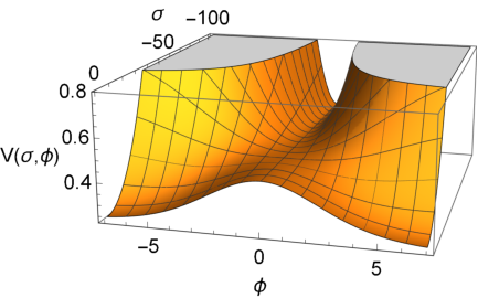
The above potential is shown in Fig. 1.
3 The modified hybrid mechanism
The first task is to investigate whether the hybrid mechanism operates as usual, under the new form of the scalar potential. It is straightforward to find
| (6) |
and
| (7) |
At the origin we have
| (8) |
where
| (9) |
Thus, we see that () provided (). Now, Eqs. (6) and (9) suggest that
| (10) |
Because , we see that, when , the term in the square brackets above is always positive. This means that the potential in the -direction has only one extremum (where ) when . Because of Eq. (8), we find that, when , the potential in the -direction has a minimum at , as in standard hybrid inflation.
Thus, we see that, provided we begin with , the system is driven to the valley at . If the inflaton potential provides a gentle slope such that the value of gradually diminishes, then at some point the inflaton decreases down to , where the effective mass of the waterfall field becomes tachyonic and we have a phase transition which terminates inflation in the -direction. The story is identical with standard hybrid inflation [25].
4 Waterfall inflation
After the phase transition, the expectation value of the waterfall field increases. As a result, the interaction term between the two fields becomes a mass term for the inflaton, which sends it to zero, which presumably also eliminates the inflaton potential , i.e. assuming . Then, Eq. (5) suggests that the potential becomes
| (11) |
As the waterfall field rolls down the above potential, is gives rise to a bout of inflation, followed by a stiff period (see next section). Without loss of generality, we assume that the waterfall field is positive.
Inflation takes place near the hilltop, with . The potential is approximated as
| (12) |
This suggests that this period of hilltop inflation ends when [28]. The penultimate equation in the above, estimates that the potential density when has decreased by a factor .
As we discuss in the next session, , which suggests that the waterfall field undergoes fast-roll inflation [29]. The reason is that, for the slow-roll parameter, we have
| (13) |
which is of order unity when . In the above, we used that at the top of the potential, where the waterfall field finds itself at the phase transition, we have
| (14) |
The total e-folds of fast-roll inflation are [29]
| (15) |
where we estimated the initial value of the waterfall field as and
| (16) |
can be large if . We can estimate as follows. The potential density on top of the hill is the same as in the valley of the hybrid potential, which is the one that drives primordial inflation along the direction. Typically, in order to obtain the correct amplitude for the curvature perturbation, the potential density of primordial inflation is . Thus we find
| (17) |
5 Waterfall stiff period
After the end of fast-roll inflation the waterfall field is released and runs down the potential slope, giving rise to a stiff period. We can approximate the scalar potential in Eq. (11) when as
| (18) |
A canonical scalar field rolling down an exponential potential of the form soon assumes an attractor solution, which corresponds to equation of state (barotropic) parameter given by (provided ) [30, 31, 32]. Thus, in our case, we expect the rolling waterfall field to be characterised by the barotropic parameter
| (19) |
The stiff period is therefore not free-fall, with and the field is not fully dominated by its kinetic energy, because in the exponential attractor evolution, all the terms of the Klein-Gordon equation of motion are comparable. However, the barotropic parameter can still be larger than 1/3.
A stiff period when results in a peak in the spectrum of gravitational waves, which are produced by primordial inflation [17]. This peak corresponds to frequencies which re-enter the horizon during the stiff period. Now, in kination when , this spike is very sharp and corresponds to high frequencies, beyond observational capabilities in the foreseeable future. If kination lasted longer, so that lower frequencies of gravitational waves can still re-enter the horizon during kination, then the peak becomes too pronounced and affects the process of Big Bang Nucleosynthesis (BBN) [23].
However, if is less than unity but still larger than the radiation value of 1/3, then the peak corresponding to the stiff period is milder. Then the stiff period can last longer, allowing primordial gravitational waves of lower frequencies to be enhanced without threatening BBN. In Ref. [24] it was shown that in the range , detectable gravitational wave frequencies are amplified such that they will be observable in the near future by LISA, without disturbing BBN. In view of Eq. (19), this range corresponds to the range , i.e. . Using Eq. (3), we find .
In the following, to help with our analytic treatment, we choose (), which corresponds to . Using this value in Eq. (17), we find . Then, Eq. (15) suggests that . Note that standard Coleman-Weinberg hybrid inflation in supergravity, when , is brought into agreement with Planck observations if there is a bout of inflation subsequent to primordial inflation [33].
6 Reheating
The density during the stiff matter period scales as , where we used the approximation . Thus, the density parameter of radiation during the stiff period is
| (20) |
Therefore, we obtain
| (21) |
where ‘end’ denotes the end of fast-roll inflation and ‘reh’ denotes the moment of reheating, when radiation becomes dominant and the Hot Big Bang begins. Using the above, we find
| (22) |
Under the simplifying assumption that , we can estimate the reheating temperature
| (23) |
where is the number of effective relativistic degrees of freedom and we used that .
In Ref. [24] it is shown that we need 1 MeVMeV for observable primordial gravitational waves.77 7 Note that the lower bound on the reheating temperature is about 4 MeV [34]. Considering MeV, Eq. (23) suggests that . It is easy to show that either gravitational particle production, or even the outburst of tachyonic fluctuations at the phase transition are not enough to generate the desired reheating efficiency.88 8 Recall that there is a period of e-folds of fast-roll inflation after the phase transition, which dilutes significantly the products of the tachyonic particle production. Therefore, another mechanism is needed for reheating. As an example, we employ Ricci reheating [35, 36, 37], which has the advantage of not introducing any additional coupling of the infaton or the waterfall to the spectator field responsible for reheating (in contrast to other mechanisms, such as instant preheating [38]). It also does not depend on initial conditions (as does curvaton reheating, for example [39, 40]).99 9 For other reheating mechanisms in NO inflation see Refs. [41, 42, 43, 44]. This is why it has been considered when modelling quintessential inflation (e.g. see Ref. [45]).
Ricci reheating considers a non-minimally coupled scalar field , with Lagrangian density
| (24) |
where , is the Ricci scalar, is the non-perturbative non-minimal coupling to gravity and the ellipsis denotes higher order terms, which can stabilise the potential of . The Ricci scalar is , where is the barotropic parameter of the Universe. During inflation, both primordial and fast-roll, we have , which means that and the non-minimal coupling generates a positive effective mass squared for the field. After the end of fast-roll inflation we have the waterfall stiff period with . As a result, and the effective mass squared of becomes tachyonic. Consequently, there is a tachyonic outburst of -particles, which eventually decay into the radiation bath of the Hot Big Bang.
Let us estimate the reheating efficiency of the process. The density of the produced radiation at the phase transition is roughly , where is the effective mass-squared of the -field and is its expectation value (squared) at the phase transition. Thus, . Then, for the reheating efficiency we find
| (25) |
During fast-roll inflation, the Hubble parameter is roughly constant so that , which is given by Eq. (14). Using the selected value of (such that ) we obtain . Demanding that and using Eq. (17) we find that .
7 The peak in the spectrum of gravitational waves
The background of primordial gravitational waves generated during inflation (primordial and/or fast-roll) acquires a spectrum given by [46]
| (26) |
where is the frequency and is the barotropic parameter of the Universe. For the modes which re-enter the horizon during the stiff period when we have . Then, the gravitational wave spectrum is
| (27) |
where ‘eq’ denotes the time of equal radiation and matter densities (equality) and ‘0’ denotes the present. In the above, is a constant which we evaluate below, where with ‘rad’ we denote the modes which re-enter the horizon during the radiation era.
The characteristic frequencies above can be estimated as follows. For a given momentum scale , the corresponding frequency is [46]
| (28) |
where the subscript ‘’ denotes the time when the scale in question re-enters the horizon after inflation.
In the case of we find . Now, we have
| (29) |
where we considered that GeV, with and . Using that , we find
| (30) |
For we consider that (cf. Eq. (28))
| (31) |
where we used Eq. (21) and that, during the stiff period we have , with , Therefore, from Eqs. (30) and (31) we obtain
| (32) |
For we find (cf. Eq. (28))
| (33) |
where we ignored dark energy and considered that y and y. Using that eV, we obtain
| (34) |
In order to estimate in Eq. (27) we need to calculate the density parameter of gravitational radiation at present. We find
| (36) |
where, during the stiff period, . Using the fact that, at the end of fast-roll inflation we have we find , where . Then, in view of Eq. (21), the above becomes
| (37) |
Now, in view of Eq. (27), we have
| (38) |
where we considered Eqs. (30), (32) and (37) and also that the integral is dominated by the high-frequency part. It is important to note here that the BBN bound is an integrated constraint.
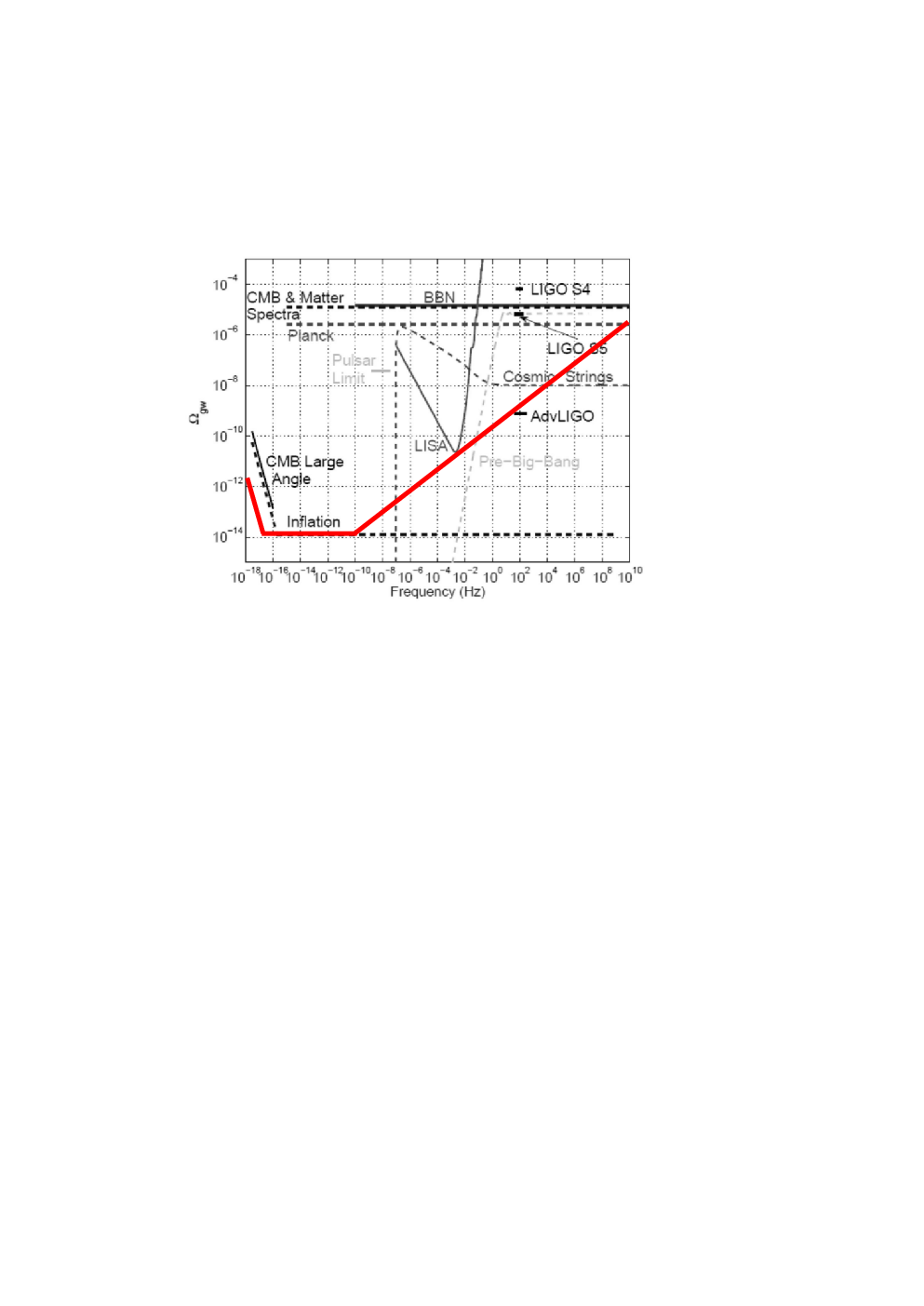
We plot Eq. (27) with in Fig. 2, using also Eqs. (30), (32), (34) and (35). It is evident that the peak in the gravitational wave spectrum is marginally observable by LISA and within reach of Advanced LIGO.1010 10 Here we are interested in order of magnitude estimates, but it must be noted that the spectral density of gravitational waves is also mildly sensitive to the effective degrees of freedom [51]. In other estimates, the sensitivity of LISA is larger after gathering enough data. As a result, as shown in Fig. 3, the peak of primordial gravitational waves is well within observability by LISA. Also, as depicted in Fig. 3, the enhanced primordial gravitational waves could be clearly seen by other future missions, such as BBO [52].

We can estimate the density parameter of gravitational waves during Big Bang Nucleosynthesis (BBN) as follows. Today, the density parameter of radiation is . Thus we find
| (39) |
where we used Eq. (37). Because we have
| (40) |
where the sub/superscript ‘BBN’ denotes the epoch of BBN. Thus, as expected saturates the bound from BBN, such that the process is not disturbed by the primordial gravitational waves.
8 Discussion
We have investigated a generic model where there is an Enhanced Symmetry Point (ESP) in field space where two flat directions are coupled. Of these, one flat direction corresponds to the inflaton field, which drives primordial inflation that resolves the fine-tuning problems of the Hot Big Bang and is responsible for the generation of the curvature perturbation, which seeds the formation of structure in the Universe. But we were interested in another aspect of primordial inflation, namely the generation of gravitational waves. The other flat direction can be a modulus field because it has a Planckian Vacuum Expectation Value (VEV). The coupling between the two gives rise to the standard hybrid mechanism [25], which terminates primordial inflation via a phase transition, when the inflaton field reaches near the ESP. After the phase transition, the system rolls along the waterfall direction, sliding off from the central potential hill, and driving a period of fast-roll hilltop inflation [29]. So far, the scenario does not differ much from many such configurations considered in the literature.
Things change when considering that the kinetic term of the waterfall field is non-trivial and features a pole at the VEV, in the manner of -attractors [26]. To assist our intuition, we switch to the canonically normalised waterfall field, for which the VEV is displaced at infinity. The hybrid scenario is not affected because near the ESP (at the top of the potential hill), the non-canonical waterfall field is approximately canonical. However, as the waterfall field slides away from the ESP, its potential is deformed and, instead of rushing towards its VEV after the end of hilltop fast-roll inflation, it follows an exponential attractor solution. This solution suggests that the equation of state of the Universe is delicately dependent on the waterfall VEV . If then the resulting equation of state is such that it drives a stiff period, with a barotropic parameter . The significance of this, is that there is a peak in the spectrum of primordial gravitational waves, such that they can be observable in the near future by LISA [24].
The fact that a peak in the spectrum of gravitational waves is generated when the Universe after inflation (which produces them) enters a stiff period, is well known [17]. However, most models which result in such a period consider a stiff phase with , dominated by the kinetic energy density of the inflaton field. This is why this period is called kination [21]. In our case, the exponential attractor solution is such that the potential and kinetic energy densities of the waterfall field are comparable, so this waterfall stiff period is not really a period of kinetic energy density domination. The significance of this is as follows.
In kination (with ), the peak in the spectrum of primordial gravitational waves is very sharp and located at too high frequencies to be observable. If kination lasted long enough to approach observable frequencies, then the peak would become so large that the total energy density in gravitational waves would disturb Big Bang Nucleosynthesis (BBN) [23], one of the pillars of the Hot Big Bang. However, when the peak inthe spectrum of gravitational waves is milder and so it can spread out to frequencies low enough to be observable without affecting BBN. We have demonstrated this in our Fig. 2.
Thus, we find that, our setup can quite naturally generate observable primordial gravitational waves. One only needs two flat directions meeting at an ESP, with one of these having a non-canonical kinetic term with a pole at its Planckian VEV . The only tuning we require so-far is that .
This is of course not enough. Achieving the largest possible growth in the spectrum of the gravitational waves, which leaves BBN unaffected, requires a reheating temperature about MeV [24]. The outburst of tachyonic perturbations at the phase transition (with original density ), which terminates primordial inflation and sends the waterfall field down its potential cannot produce enough radiation to reheat the Universe this early. Thus, we have to consider alternative reheating mechanisms. Many such mechanisms have been considered in models of quintessential inflation, which feature a kination period [41]. As an example, we employed the Ricci reheating mechanism [35, 36, 37], which considers the influence of a non-minimal spectator scalar field, whose effective mass squared changes sign at the end of hilltop fast-roll inflation (not at the phase transition) producing an outburst of tachyonic perturbations with original density . We have shown that we obtain enough radiation to achieve the desired reheating temperature when the non-minimal coupling is ; a very reasonable value.
One possible criticism of the above scenario is that the excursion of the canonical field is super-Planckian and this would result in radiative corrections which could lift the flatness of the waterfall potential after the end of the fast-roll hilltop inflation phase. A super-Planckian excursion of the field might result also in a sizeable 5th-force problem, which could violate the Principle of Equivalence. Of course, the interaction terms in the Lagrangian density of the theory are of the form [47], where is any gauge-invariant dimension-four operator (for example for electromagnetism ), and are some constants of order unity. Crucially, this expression features the non-canonical waterfall field , whose excursion is only Planckian, since its VEV is . Thus, we only need to suppress radiative corrections and the 5th force problem. Still, one could consider this as substantial fine tuning because the are many. A better argument can be made if we take seriously the Ricci reheating mechanism. In this mechanism, the thermal bath of the Hot Big Bang is solely due to the decay products of the spectator field , which is not coupled to either the inflaton or the waterfall field .1111 11 In fact, could conceivably be the Higgs field itself. As a result, we may consider that both and are completely uncoupled to the standard model and belong to a dark sector. As such, they do not cause any violation to the Equivalence Principle.1212 12 A similar argument can be made for the curvaton reheating mechanism. As far as the radiative corrections are concerned, they could simply be responsible for generating the Planckian VEV of .
Even so, it may be argued that, when the waterfall field approaches its Planckian VEV, the perturbative form of the potential in Eq. (1) is questionable. Firstly, the waterfall field approaches is VEV asymptotically, when for the canonical waterfall field . This implies that any deformations of the potential until reheating (afterwards it is negligible) are expected to be mild. As such, the estimated values of the model parameters , and might be somewhat affected, but we do not expect this to be substantial.
Another potential issue has to do with the phase transition, which terminates inflation and sends the waterfall field down the hilltop of its potential. It can be argued that modelling the system as a rolling ball is not applicable in this case, because the phase transition is non-perturbative. As such, the validity of Eq. (15) could be undermined. However, investigating the phase transition at the onset of fast-roll inflation in the appropriate detail, produces very similar results as with our simple treatment here [48].1313 13 A recent study of the backreaction of waterfall fluctuations on the inflaton field at the phase transition, showed that the curvature of the potential in the inflaton direction must be substantial, while the strength of the ESP not too large (so ), for the classical approximation to be valid [49]. This depends on the choice of and the inflaton potential , which we assume to be such that the aforementioned backreaction is not strong. A related issue is of possible topological defects generated at the phase transition. Firstly, there are e-folds of fast roll inflation following the phase transition, which would dilute somewhat any topological defects. The kind of topological defects created has to do with the nature of the waterfall field. For example, if is complex, we expect the formation of cosmic strings, which could be made harmless if they are unstable.

Finally, let us consider what happens to the waterfall field after reheating. Once the Universe becomes dominated by some substance other than the scalar field, the exponential attractor changes and becomes such that the density of the rolling scalar field mimics the background (whatever this is) and stays at a constant ratio [31, 32]. In our case, this ratio is given by , where . Does this mean that we cannot help but affect BBN after all, since the Universe content would contain in effect an extra relativistic species? (the barotropic parameter of the scalar field mimics that of the background, i.e. during the radiation era.) There is hope that we escape this danger, but only because reheating occurs close to BBN. Then, as the Universe expansion changes rate, we expect that the scalar field would overshoot the subdominant attractor [32] and there will be some limited period of time, when its contribution to the density budget of the Universe is small enough to avoid disturbing BBN. This is possible only because reheating is so close to BBN. Pictorially, this overshooting is depicted in Fig. 4. Soon after BBN, the field is expected to assume the subdominant exponential attractor. Therefore, in the matter era, we expect that it comprises a large fraction of dark matter. Needless to say that all the above warrant a detailed numerical investigation, which we will do in a subsequent paper.
9 Conclusions
All in all, we have presented a toy-model of hybrid inflation, where the waterfall field has a non-canonical kinetic term which features a pole at its Planckian VEV. In this case, we have argued that, after inflation there is a stiff period such that the corresponding primordial gravitational waves can be enhanced enough to be observable by LISA and Advanced LIGO without disturbing BBN.
Acknowledgements
I am thankful to Samuel Sánchez López for his help regarding Fig. 1 and to the anonymous referee, who made me realise that the observability of the gravitational waves in the scenario presented is greater than I originally thought. This work was supported, in part, by the Lancaster-Manchester-Sheffield Consortium for Fundamental Physics under STFC grant: ST/T001038/1.
References
- [1] A. A. Starobinsky, Phys. Lett. B 91 (1980) 99.
- [2] A. H. Guth, Phys. Rev. D 23 (1981) 347.
- [3] D. Kazanas, Astrophys. J. Lett. 241 (1980), L59-L63.
- [4] K. Sato, Mon. Not. Roy. Astron. Soc. 195 (1981), 467-479.
- [5] L. Perivolaropoulos, Nucl. Phys. B Proc. Suppl. 148 (2005), 128-140 [arXiv:astro-ph/0501590 [astro-ph]].
- [6] A. R. Liddle and D. H. Lyth, “Cosmological inflation and large scale structure,” Cambridge, UK: Univ. Pr. (2000) 400 pp.
- [7] M. S. Turner, Phys. Rev. D 55 (1997), R435-R439 [arXiv:astro-ph/9607066 [astro-ph]].
- [8] J. Aasi et al. [LIGO Scientific], Class. Quant. Grav. 32 (2015), 074001 [arXiv:1411.4547 [gr-qc]].
- [9] F. Acernese et al. [VIRGO], Class. Quant. Grav. 32 (2015) no.2, 024001 [arXiv:1408.3978 [gr-qc]].
- [10] P. Amaro-Seoane et al. [LISA], [arXiv:1702.00786 [astro-ph.IM]].
- [11] R. Abbott et al. [KAGRA, Virgo and LIGO Scientific], Phys. Rev. D 104 (2021) no.2, 022004 [arXiv:2101.12130 [gr-qc]].
- [12] G. N. Felder, L. Kofman and A. D. Linde, Phys. Rev. D 60 (1999), 103505 [arXiv:hep-ph/9903350 [hep-ph]].
- [13] P. J. E. Peebles and A. Vilenkin, Phys. Rev. D 59 (1999), 063505 [arXiv:astro-ph/9810509 [astro-ph]].
- [14] N. Jaman and M. Sami, Galaxies 10 (2022) no.2, 51 [arXiv:2202.06194 [gr-qc]].
- [15] J. de Haro and L. A. Saló, Galaxies 9 (2021) no.4, 73 doi:10.3390/galaxies9040073 [arXiv:2108.11144 [gr-qc]].
- [16] L. P. Grishchuk and Y. V. Sidorov, Phys. Rev. D 42 (1990), 3413-3421.
- [17] V. Sahni, M. Sami and T. Souradeep, Phys. Rev. D 65 (2002), 023518 [arXiv:gr-qc/0105121 [gr-qc]].
- [18] L. A. Boyle and P. J. Steinhardt, Phys. Rev. D 77 (2008), 063504 [arXiv:astro-ph/0512014 [astro-ph]].
- [19] S. Kuroyanagi, K. Nakayama and S. Saito, Phys. Rev. D 84 (2011), 123513 [arXiv:1110.4169 [astro-ph.CO]].
- [20] T. L. Smith, M. Kamionkowski and A. Cooray, Phys. Rev. D 73 (2006), 023504 [arXiv:astro-ph/0506422 [astro-ph]].
- [21] M. Joyce and T. Prokopec, Phys. Rev. D 57 (1998), 6022-6049 [arXiv:hep-ph/9709320 [hep-ph]].
- [22] B. Li and P. R. Shapiro, JCAP 10 (2021), 024 [arXiv:2107.12229 [astro-ph.CO]].
- [23] J. H. Cases and L. Aresté Saló, Universe 6 (2020) no.6, 87 [arXiv:2004.11843 [gr-qc]].
- [24] D. G. Figueroa and E. H. Tanin, JCAP 08 (2019), 011 [arXiv:1905.11960 [astro-ph.CO]].
- [25] A. D. Linde, Phys. Rev. D 49 (1994), 748-754 [arXiv:astro-ph/9307002 [astro-ph]].
- [26] R. Kallosh, A. Linde and D. Roest, JHEP 11 (2013), 198 [arXiv:1311.0472 [hep-th]].
- [27] R. Kallosh and A. Linde, [arXiv:2204.02425 [hep-th]].
- [28] L. Boubekeur and D. H. Lyth, JCAP 07 (2005), 010 [arXiv:hep-ph/0502047 [hep-ph]].
- [29] A. D. Linde, JHEP 11 (2001), 052 [arXiv:hep-th/0110195 [hep-th]].
- [30] F. Lucchin and S. Matarrese, Phys. Rev. D 32 (1985), 1316.
- [31] E. J. Copeland, A. R. Liddle and D. Wands, Phys. Rev. D 57 (1998), 4686-4690 [arXiv:gr-qc/9711068 [gr-qc]].
- [32] K. Dimopoulos, “Introduction to Cosmic Inflation and Dark Energy,” CRC Press (Taylor & Francis) (2021) 280pp.
- [33] K. Dimopoulos and C. Owen, JCAP 10 (2016), 020 [arXiv:1606.06677 [hep-ph]].
- [34] T. Hasegawa, N. Hiroshima, K. Kohri, R. S. L. Hansen, T. Tram and S. Hannestad, JCAP 12 (2019), 012 [arXiv:1908.10189 [hep-ph]].
- [35] K. Dimopoulos and T. Markkanen, JCAP 06 (2018), 021 [arXiv:1803.07399 [gr-qc]].
- [36] T. Opferkuch, P. Schwaller and B. A. Stefanek, JCAP 07 (2019), 016 [arXiv:1905.06823 [gr-qc]].
- [37] D. Bettoni, A. Lopez-Eiguren and J. Rubio, JCAP 01 (2022) no.01, 002 [arXiv:2107.09671 [hep-ph]].
- [38] G. N. Felder, L. Kofman and A. D. Linde, Phys. Rev. D 59 (1999), 123523 [arXiv:hep-ph/9812289 [hep-ph]].
- [39] B. Feng and M. z. Li, Phys. Lett. B 564 (2003), 169-174 [arXiv:hep-ph/0212213 [hep-ph]].
- [40] J. C. Bueno Sanchez and K. Dimopoulos, JCAP 11 (2007), 007 [arXiv:0707.3967 [hep-ph]].
- [41] J. Haro, Phys. Rev. D 99 (2019) no.4, 043510 [arXiv:1807.07367 [gr-qc]].
- [42] H. Tashiro, T. Chiba and M. Sasaki, Class. Quant. Grav. 21 (2004), 1761-1772 [arXiv:gr-qc/0307068 [gr-qc]].
- [43] K. Dimopoulos and L. Donaldson-Wood, Phys. Lett. B 796 (2019), 26-31 [arXiv:1906.09648 [gr-qc]].
- [44] I. Dalianis and G. P. Kodaxis, Galaxies 10 (2022) no.1, 31 [arXiv:2112.15576 [astro-ph.CO]].
- [45] K. Dimopoulos, A. Karam, S. Sánchez López and E. Tomberg, Galaxies 10 (2022) no.2, 57 doi:10.3390/galaxies10020057 [arXiv:2203.05424 [gr-qc]].
- [46] Y. Gouttenoire, G. Servant and P. Simakachorn, [arXiv:2111.01150 [hep-ph]].
- [47] S. M. Carroll, Phys. Rev. Lett. 81 (1998), 3067-3070 [arXiv:astro-ph/9806099 [astro-ph]].
- [48] K. Dimopoulos, T. Markkanen, A. Racioppi and V. Vaskonen, JCAP 07 (2019), 046 [arXiv:1903.09598 [astro-ph.CO]].
- [49] J. O. Gong and M. Mylova, [arXiv:2202.13882 [hep-th]].
- [50] E. Thrane and J. D. Romano, Phys. Rev. D 88 (2013) no.12, 124032 [arXiv:1310.5300 [astro-ph.IM]].
- [51] Y. Watanabe and E. Komatsu, Phys. Rev. D 73 (2006), 123515 [arXiv:astro-ph/0604176 [astro-ph]].
- [52] G. M. Harry, P. Fritschel, D. A. Shaddock, W. Folkner and E. S. Phinney, Class. Quant. Grav. 23 (2006), 4887-4894 [erratum: Class. Quant. Grav. 23 (2006), 7361].