跳到论文正文
W Papers独立论文阅读器 arXiv:2206.01891 论文正文 计算阅读时间 · 0%
引用这篇论文根据当前论文元数据生成,正式投稿前建议核对。


License: arXiv.org perpetual non-exclusive license
arXiv:2206.01891v1 [eess.SP] 04 Jun 2022

8D Parameters Estimation for Bistatic EMVS-MIMO Radar via the nested PARAFAC

Qianpeng Xie    He Wang    Yihang Du    Xiaoyi Pan    Feng Zhao Thanks:  This work was supported in part by the National Natural Science Foundation of China under Grant 61890545, 61890542 and 61890540. Thanks: Qianpeng Xie, Xiaoyi Pan, Feng Zhao are with the State Key Laboratory of Complex Electromagnetic Environment Effects on Electronics and Information System, National University of Defense Technology, Changsha 410073, China(email:13721038905@163.com, mrpanxy@nudt.edu.cn, zhfbee@tom.com).He Wang is with the School of Electronic Science, National University of Defense Technology, Changsha 410073, China.(email:hw8g16@soton.ac.uk).Yihang Du is with the Sixty-Third Research Institute, National University of Defense Technology, Nanjing 210007, China(email:dyhcsl1991@163.com). (Corresponding author: Qianpeng Xie ).
Abstract

In this letter, a novel nested PARAFAC algorithm was proposed to improve the 8D parameters estimation performance for the bistatic EMVS-MIMO radar. Firstly, the outer part PARAFAC algorithm was carried out to estimate the receive spatial response matrix and its first way factor matrix. For the estimated first way factor matrix, a theory is given to rearrange its data into an new matrix, which is the mode-1 unfolding matrix of a three-way tensor. Then, the inner part PARAFAC algorithm was used to estimate the transmit steering vector matrix, the transmit spatial response matrix and the receive steering vector matrix. Thus, the transmit 4D parameters and receive 4D parameters can be accurately located via the abovementioned process. Compared with the original PARAFAC algorithm, the proposed nested PARAFAC algorithm can avoid additional reconstruction process when estimating the transmit/receive spatial response matrix. Moreover, the proposed algorithm can offer a highly-accurate 8D parameters estimaiton than that of the original PARAFAC algorithm. Simulated results verify the effectiveness of the proposed algorithm.

Index Terms: 
Bistatic EMVS-MIMO radar, nested PARAFAC algorithm, tensor model, parameters estimation

I Introduction

Recently, the research about the electromagnetic vector sensors (EMVS) has attracted extensive attention due to its excellent measurement capabilities of angle parameters and polarization parameters [1]-[5]. In order to estimate the polarization parameters in bistatic EMVS-MIMO radar, the ESPRIT algorithm was firstly proposed in [6]. The significance of the ESPRIT algorithm is to derive a method to reconstruct the transmit/receive spatial response matrix, but its computational complexity is large. In order to reduce the computational complexity, the PM algorithm was proposed in [7], which can estimate the signal subspace matrix by avoiding the singular value decomposition process of the covariance matrix. To make full use of the space-time multidimensional structure of the array received data, the HOSVD algorithm based on the fourth-order tensor was raised in [8]. However, the algorithms reported in [6]-[8] need the pair matching process for the 2D-DOD and 2D-DOA estimation. Therefore, a modified PM algorithm in [9] and PARAFAC algorithm in [10] were proposed to realize the 2D-DOD and 2D-DOA automatically paired. In [11], the bistatic coprime EMVS-MIMO radar was designed to improve the 2D-DOD and 2D-DOA estimaiton performance.

Through analysis, it can be found that the above mentioned algorithms can be used to estimate the 8D parameters in bistatic EMVS-MIMO radar. Amongst, the HOSVD algorithm can offer the best estimation performance, but its shortcoming is the high computational load. The modified PM algorithm and the PARAFAC algorithm can realize the 2D-DOD and 2D-DOA automatically paired. But, the estimation performance of them are relatively poor. According to [12]-[13], the nested PARAFAC algorithm can improve the estimation performance of the angle parameter, but, it cannot be directly used in the bistatic EMVS-MIMO radar due to the special structure of the receive data. Motivated by the strategy in [12]-[13], we proposed a new nested PARAFAC algorithm. Firstly, the outer part PARAFAC was conducted to estimate the receive spatial response and the first way factor matrix. Then, the inner part three way tensor can be constructed by rearranging the estimated first way factor matrix, which can be used to estimate transmit steering vector matrix, transmit spatial response matrix and the receive steering vector matrix. Compared with the HOSVD algorithm, the raised new nested PARAFAC algorithm has lower computational complexity. And this method presents a higher estimation accuracy than the original PARAFAC algorithm as well as the modified PM algorithm.

II DATA MODEL

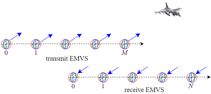
As shown in Fig. 1, for a bistatic EMVS-MIMO radar system consists of MM transmit EMVS and NN receive EMVS, the transmit steering vector and receive steering vector can be expressed as
Refer to caption

Fig. 1: Bistatic EMVS-MIMO radar system
𝒄tk=𝒂tk⊗𝒒tk​(θtk,ϕtk,γtk,ηtk)\displaystyle\boldsymbol{c}_{t_{k}}=\boldsymbol{a}_{t_{k}}\otimes\boldsymbol{q}_{t_{k}}(\theta_{t_{k}},\phi_{t_{k}},\gamma_{t_{k}},\eta_{t_{k}}) (1)
𝒄rk=𝒂rk⊗𝒒rk​(θrk,ϕrk,γrk,ηrk)\displaystyle\boldsymbol{c}_{r_{k}}=\boldsymbol{a}_{r_{k}}\otimes\boldsymbol{q}_{r_{k}}(\theta_{r_{k}},\phi_{r_{k}},\gamma_{r_{k}},\eta_{r_{k}}) (2)

where k=1,2,…,Kk=1,2,\dots,K denote the number of targets, θtk,θrk∈[0,π)\theta_{t_{k}},\theta_{r_{k}}\in[0,\pi), ϕtk,ϕrk∈[0,2​π)\phi_{t_{k}},\phi_{r_{k}}\in[0,2\pi), γtk,γrk∈[0,π/2)\gamma_{t_{k}},\gamma_{r_{k}}\in[0,\pi/2) and ηtk,ηrk∈[−π,π)\eta_{t_{k}},\eta_{r_{k}}\in[-\pi,\pi) denote the transmit/receive elevation angle, transmit/receive azimuth angle, transmit/receive polarization angle and transmit/receive polarization phase difference, respectively. 𝒒tk​(θtk,ϕtk,γtk,ηtk)\boldsymbol{q}_{t_{k}}(\theta_{t_{k}},\phi_{t_{k}},\gamma_{t_{k}},\eta_{t_{k}}) and 𝒒rk​(θrk,ϕrk,γrk,ηrk)\boldsymbol{q}_{r_{k}}(\theta_{r_{k}},\phi_{r_{k}},\gamma_{r_{k}},\eta_{r_{k}}) represent the spatial response of the transmit EMVS and the receive EMVS of the kk-th target. 𝒂tk=[e−j​π​sin⁡(θtk),e−j​π​2​sin⁡(θtk),⋯,e−j​π​M​sin⁡(θtk)]T{\boldsymbol{a}_{t_{k}}=}{[e^{-j\pi\sin(\theta_{t_{k}})},e^{-j\pi 2\sin(\theta_{t_{k}})},\cdots,e^{-j\pi M\sin(\theta_{t_{k}})}]^{T}}, 𝒂rk={\boldsymbol{a}_{r_{k}}}{=} [e−j​π​sin⁡(θrk),e−j​π​2​sin⁡(θrk),⋯,e−j​π​N​sin⁡(θrk)]T{[e^{-j\pi\sin(\theta_{r_{k}})},e^{-j\pi 2\sin(\theta_{r_{k}})},\cdots,e^{-j\pi N\sin(\theta_{r_{k}})}]^{T}}. Accodring to [1], the spatial response 𝒒\boldsymbol{q} of an EMVS can be expressed as

𝒒⁡(θ,ϕ,γ,η)=\displaystyle\boldsymbol{q}(\theta,\phi,\gamma,\eta)= (3)
[cos⁡(ϕ)​cos⁡(θ)−sin⁡(ϕ)sin⁡(ϕ)​cos⁡(θ)cos⁡(ϕ)−sin⁡(θ)0−sin⁡(ϕ)−cos⁡(ϕ)​cos⁡(θ)cos⁡(ϕ)−sin⁡(ϕ)​cos⁡(θ)0sin⁡(θ)]⏟𝑭⁡(θ,ϕ)​[sin⁡(γ)​ej​ηcos⁡(γ)]⏟𝒈⁡(γ,ηCLOSE\displaystyle\underbrace{\begin{bmatrix}\cos(\phi)\cos(\theta)&-\sin(\phi)\\ \sin(\phi)\cos(\theta)&\cos(\phi)\\ -\sin(\theta)&0\\ -\sin(\phi)&-\cos(\phi)\cos(\theta)\\ \cos(\phi)&-\sin(\phi)\cos(\theta)\\ 0&\sin(\theta)\\ \end{bmatrix}}_{\boldsymbol{F}(\theta,\phi)}\underbrace{\begin{bmatrix}\sin(\gamma)e^{j\eta}\\ \cos(\gamma)\\ \end{bmatrix}}_{\boldsymbol{g}(\gamma,\eta}

where 𝑭⁡(θ,ϕ)∈ℂ6×2{\boldsymbol{F}(\theta,\phi)}\in\mathbb{C}^{6\times 2} denotes the spatial angular location matrix , 𝒈⁡(γ,η)∈ℂ2×1{\boldsymbol{g}(\gamma,\eta)}\in\mathbb{C}^{2\times 1} denotes the polarization states vector.

The data model at the receive front can be expressed as

𝒚⁡(t)\displaystyle\boldsymbol{y}(t) =[(𝑨t⊙𝑸t)⊙(𝑨r⊙𝑸r)]​𝒔​(t)+𝒏⁡(t)\displaystyle=\left[(\boldsymbol{A}_{t}\odot\boldsymbol{Q}_{t})\odot(\boldsymbol{A}_{r}\odot\boldsymbol{Q}_{r})\right]\boldsymbol{s}(t)+\boldsymbol{n}(t) (4)

where 𝑨t=[𝒂t1,𝒂t2,⋯,𝒂tK]\boldsymbol{A}_{t}=\left[\boldsymbol{a}_{t_{1}},\boldsymbol{a}_{t_{2}},\cdots,\boldsymbol{a}_{t_{K}}\right], 𝑨r=[𝒂r1,𝒂r2,⋯,\boldsymbol{A}_{r}=[\boldsymbol{a}_{r_{1}},\boldsymbol{a}_{r_{2}},\cdots, 𝒂rK]\boldsymbol{a}_{r_{K}}], 𝑸t=[𝒒t1,𝒒t2,⋯,𝒒tK]\boldsymbol{Q}_{t}=\left[\boldsymbol{q}_{t_{1}},\boldsymbol{q}_{t_{2}},\cdots,\boldsymbol{q}_{t_{K}}\right] and 𝑸r=[𝒒r1,𝒒r2CLOSE,\boldsymbol{Q}_{r}=[\boldsymbol{q}_{r_{1}},\boldsymbol{q}_{r_{2}}, OPEN⋯,𝒒rK]\cdots,\boldsymbol{q}_{r_{K}}] denote the transmit steering matrix, the receive steering matrix, the transmit spatial response matrix and the receive spatial response matrix, respectively. For the total LL snapshots, the sample data can be further expressed written as

𝒀\displaystyle\boldsymbol{Y} =[(𝑨t⊙𝑸t)⊙(𝑨r⊙𝑸r)]​𝑺+𝑵\displaystyle=\left[(\boldsymbol{A}_{t}\odot\boldsymbol{Q}_{t})\odot(\boldsymbol{A}_{r}\odot\boldsymbol{Q}_{r})\right]\boldsymbol{S}+\boldsymbol{N} (5)

III The proposed strategy

III-A The nested PARAFAC algorithm

In order to reserve the mutiple space-time structure in 𝒀\boldsymbol{Y}, a nested-tensor signal model are designed as follows

𝒀\displaystyle\boldsymbol{Y} =[(𝑨t⊙𝑸t)⊙(𝑨r⊙𝑸r)]​𝑺+𝑵\displaystyle=\left[\left(\boldsymbol{A}_{t}\odot\boldsymbol{Q}_{t}\right)\odot\left(\boldsymbol{A}_{r}\odot\boldsymbol{Q}_{r}\right)\right]\boldsymbol{S}+\boldsymbol{N} (6)
=[(𝑨t⊙𝑸t⊙𝑨r)⏞i​n​n​e​r​p​a​r​t⊙𝑸r]​𝑺+𝑵⏟o​u​t​e​r​p​a​r​t\displaystyle=\underbrace{\left[\overbrace{\left(\boldsymbol{A}_{t}\odot\boldsymbol{Q}_{t}\odot\boldsymbol{A}_{r}\right)}^{inner\hskip 8.19447ptpart}\odot\boldsymbol{Q}_{r}\right]\boldsymbol{S}+\boldsymbol{N}}_{outer\hskip 8.19447ptpart}
=[𝑨t​q​r⊙𝑸r]​𝑺+𝑵\displaystyle=\left[\boldsymbol{A}_{tqr}\odot\boldsymbol{Q}_{r}\right]\boldsymbol{S}+\boldsymbol{N}

where 𝑨t​q​r=(𝑨~t⊙𝑸t⊙𝑨~r)∈ℂ6​M​N×K\boldsymbol{A}_{tqr}=\left(\boldsymbol{\tilde{A}}_{t}\odot\boldsymbol{Q}_{t}\odot\boldsymbol{\tilde{A}}_{r}\right)\in\mathbb{C}^{6MN\times K}. Firstly, the outer part PARAFAC algorithm is used to estimate the factor matrices 𝑨t​q​r\boldsymbol{A}_{tqr} and 𝑸r\boldsymbol{Q}_{r}. According to (6), a 3-D tensor 𝒴\mathcal{Y} can be constructed as

𝒴\displaystyle\mathcal{Y} =∑k=1K𝒂t​q​r∘𝒒r∘𝒔T+𝒩\displaystyle=\sum_{k=1}^{K}\boldsymbol{a}_{tqr}\circ\boldsymbol{q}_{r}\circ\boldsymbol{s}^{T}+\mathcal{N} (7)

The different silices of the third-order tensor 𝒴\mathcal{Y} can be further expressed as

𝒴T[i,:,:]\displaystyle\mathcal{Y}^{T}_{[{i,:,:}]} =𝑸r𝒟i(𝑺T)𝑨Tt​q​r,i=1,2,⋯,L\displaystyle=\boldsymbol{Q}_{r}\mathcal{D}_{i}({\boldsymbol{S}}^{T})\boldsymbol{A}^{T}_{tqr},\quad i=1,2,\cdots,L (8)
𝒴T[:,j,:]\displaystyle\mathcal{Y}^{T}_{[{:,j,:}]} =𝑺T𝒟j(𝑨𝒕​𝒒​𝒓)𝑸rT,j=1,2,⋯,6MN\displaystyle=\boldsymbol{S}^{T}\mathcal{D}_{j}({{\boldsymbol{{A}_{tqr}}}})\boldsymbol{Q}_{r}^{T},\quad j=1,2,\cdots,6{MN}
𝒴T[:,:,k]\displaystyle\mathcal{Y}^{T}_{[{:,:,k}]} =𝑨t​q​r𝒟k(𝑸r)𝑺,k=1,2,⋯,6\displaystyle=\boldsymbol{A}_{tqr}\mathcal{D}_{k}(\boldsymbol{Q}_{r})\boldsymbol{S},\quad k=1,2,\cdots,6

where 𝒟i\mathcal{D}_{i}, 𝒟j\mathcal{D}_{j}, 𝒟k\mathcal{D}_{k} represent the diagonal matrix operation, and the elements on the diagonal matrices are the kk-rows of the factor matrices 𝑸r\boldsymbol{Q}_{r}, 𝑨t​q​r\boldsymbol{A}_{tqr}, and 𝑺{\boldsymbol{S}}, respectively.

In order to realize the estimation of the factor matrices 𝑸r\boldsymbol{Q}_{r}, 𝑨t​q​r\boldsymbol{A}_{tqr}, and 𝑺{\boldsymbol{S}}, the trilinear alternating least squares algorithm is used

min𝑨t​q​rT\displaystyle\min_{{\boldsymbol{A}^{T}_{tqr}}} =‖[𝒴](1)T−(𝑸r⊙𝑺T)​𝑨t​q​rT‖F2\displaystyle=\|[\mathcal{Y}]^{T}_{(1)}-\left(\boldsymbol{Q}_{r}\odot{\boldsymbol{S}}^{T}\right)\boldsymbol{A}^{T}_{tqr}\|^{2}_{F} (9)
min𝑸rT\displaystyle\min_{{\boldsymbol{Q}^{T}_{r}}} =‖[𝒴](2)T−(𝑺T⊙𝑨𝒕​𝒒​𝒓)​𝑸rT‖F2\displaystyle=\|[\mathcal{Y}]^{T}_{(2)}-\left(\boldsymbol{S}^{T}\odot{{\boldsymbol{{A}_{tqr}}}}\right)\boldsymbol{Q}_{r}^{T}\|^{2}_{F}
min𝑺\displaystyle\min_{{\boldsymbol{S}}} =‖[𝒴](3)T−(𝑨t​q​r⊙𝑸r)​𝑺‖F2\displaystyle=\|[\mathcal{Y}]^{T}_{(3)}-\left(\boldsymbol{A}_{tqr}\odot\boldsymbol{Q}_{r}\right)\boldsymbol{S}\|^{2}_{F}

Then, let 𝑺˘{{\boldsymbol{\breve{S}}}}, 𝑸˘r{\boldsymbol{\breve{Q}}_{r}} and 𝑨˘t​q​r{\boldsymbol{\breve{A}}_{tqr}} denote the estimated factor matrices, respectively

𝑨˘t​q​rT=(𝑸˘r⊙𝑺˘T)†​[𝒴](1)T\displaystyle{\displaystyle\boldsymbol{\breve{A}}^{T}_{tqr}}=({\boldsymbol{\breve{Q}}_{r}}\odot{\boldsymbol{\breve{S}}^{T}})^{\dagger}[\mathcal{Y}]^{T}_{(1)} (10)
𝑸˘rT=(𝑺˘T⊙𝑨˘t​q​r)†​[𝒴](2)T\displaystyle{{\displaystyle\boldsymbol{\breve{Q}}^{T}_{r}}}=({\boldsymbol{\breve{S}}}^{T}\odot{\boldsymbol{\breve{A}}_{tqr}})^{\dagger}[\mathcal{Y}]^{T}_{(2)}
𝑺˘=(𝑨˘t​q​r⊙𝑸˘r)†​[𝒴](3)T\displaystyle{{\displaystyle\boldsymbol{\breve{S}}}}=(\boldsymbol{\breve{A}}_{tqr}\odot{\boldsymbol{\breve{Q}}_{r}})^{\dagger}[\mathcal{Y}]^{T}_{(3)}

It can be found that the factor matrices 𝑸˘r{\boldsymbol{\breve{Q}}_{r}} and 𝑨˘t​q​r{\boldsymbol{\breve{A}}_{tqr}} can be obtained. And, the receive elevation angle, receive azimuth angle, receive polarization angle and receive polarization phase difference can be estimated by performing the vector-cross-product operation on 𝑸˘r{\boldsymbol{\breve{Q}}_{r}}.

Then, in order to estimate the transmit 4D parameters, the inter part in (6) needs to be considered. It is invalid to direct to perform inner-part PARAFAC on estimated 𝑨˘t​q​r{\boldsymbol{\breve{A}}_{tqr}}. Under this circumstance, a new three way tensor should be constructed as follows

𝒴1\displaystyle\mathcal{Y}_{1} =∑k=1K𝑨r∘𝒒t∘𝑨t\displaystyle=\sum_{k=1}^{K}\boldsymbol{A}_{r}\circ\boldsymbol{q}_{t}\circ\boldsymbol{A}_{t} (11)

However, the factor matrix 𝑨˘t​q​r≠𝒴1​(i),i=1,2,3{\boldsymbol{\breve{A}}_{tqr}}\neq\mathcal{Y}_{1{\left(i\right)}},i=1,2,3. Thus, the conversion of the factor matrix 𝑨˘t​q​r{\boldsymbol{\breve{A}}_{tqr}} into the mode-i,i=1,2,3i,i=1,2,3 unfolding of the tensor 𝒴1\mathcal{Y}_{1} is necessary. By analysis, the relationship 𝑨t​q​r\boldsymbol{A}_{tqr} and 𝒴1​(1)\mathcal{Y}_{1{\left(1\right)}}is considered. The detailed form of the mode-11 unfolding of the tensor 𝒴1\mathcal{Y}_{1} is

𝑨t​q​r^=[𝒴1](1)T=[𝑸t⊙𝑨t]​𝑨rT∈ℂ6​M×N\displaystyle\widehat{\boldsymbol{A}_{tqr}}=\left[\mathcal{Y}_{1}\right]^{T}_{{\left(1\right)}}=\left[{\boldsymbol{{Q}}_{t}}\odot{\boldsymbol{{A}}_{t}}\right]{\boldsymbol{{A}}^{T}_{r}}\in\mathbb{C}^{6M\times N} (12)

Here, we give an theory to show how to rearrange the factor matrix 𝑨t​q​r\boldsymbol{A}_{tqr} into the matrix 𝑨t​q​r^\widehat{\boldsymbol{A}_{tqr}}

𝑇ℎ𝑒𝑜𝑟𝑒𝑚1{\mathit{Theorem\hskip 10.22217pt1}} The matrix 𝑨t​q​r^∈ℂ6​M×N\widehat{\boldsymbol{A}_{tqr}}\in\mathbb{C}^{6M\times N} is equal to the inverse matrix vectorization by row of the vector [∑k=1K𝑨t​q​r(:,k)]∈ℂ6​M​N×1\left[\sum_{k=1}^{K}\boldsymbol{A}_{tqr}\left(:,k\right)\right]\in\mathbb{C}^{6MN\times 1}, namely

𝑨t​q​r^=ivec[∑k=1K𝑨t​q​r(:,k)]\displaystyle\widehat{\boldsymbol{A}_{tqr}}=ivec\left[\sum_{k=1}^{K}\boldsymbol{A}_{tqr}\left(:,k\right)\right] (13)

where i​v​e​civec denotes the inverse matrix vectorization by row.

𝑃𝑟𝑜𝑜𝑓:{\mathit{Proof}}: The conclusion is a direct result of the following equalities

[∑k=1K𝑨t​q​r(:,k)]\displaystyle\left[\sum_{k=1}^{K}\boldsymbol{A}_{tqr}\left(:,k\right)\right] ⇔∑k=1K(𝑨t(:,k)⊙𝑸t(:,k)⊙𝑨r(:,k))\displaystyle\Leftrightarrow\sum_{k=1}^{K}\left(\boldsymbol{A}_{t}\left(:,k\right)\odot\boldsymbol{Q}_{t}\left(:,k\right)\odot\boldsymbol{A}_{r}\left(:,k\right)\right) (14)
⇔∑k=1K(𝒂t​k⊗𝒒t​k⊗𝒂r​k)\displaystyle\Leftrightarrow\sum_{k=1}^{K}\left(\boldsymbol{a}_{tk}\otimes\boldsymbol{q}_{tk}\otimes\boldsymbol{a}_{rk}\right)
⇔1​∑k=1Kv​e​c​(𝒂r​k​(𝒂t​k⊗𝒒t​k)T)\displaystyle\overset{1}{\Leftrightarrow}\sum_{k=1}^{K}vec\left(\boldsymbol{a}_{rk}\left(\boldsymbol{a}_{tk}\otimes\boldsymbol{q}_{tk}\right)^{T}\right)
⇔2​v​e​c​(𝑨r​(𝑨t⊙𝑸t)T)\displaystyle\overset{2}{\Leftrightarrow}vec\left(\boldsymbol{A}_{r}\left(\boldsymbol{A}_{t}\odot\boldsymbol{Q}_{t}\right)^{T}\right)
⇔v​e​c​([(𝑸t⊙𝑨t)​𝑨rT]T)\displaystyle\Leftrightarrow vec\left(\left[\left({\boldsymbol{{Q}}_{t}}\odot{\boldsymbol{{A}}_{t}}\right){\boldsymbol{{A}}^{T}_{r}}\right]^{T}\right)
⇔v​e​c​((𝑨t​q​r^)T)\displaystyle\Leftrightarrow vec\left(\left(\widehat{\boldsymbol{A}_{tqr}}\right)^{T}\right)

where the ⇔1\overset{1}{\Leftrightarrow} is satisfied by using the relationship between kronecker product and vectorization of two vector 𝒂⊗𝒃=𝒂⊙𝒃=v​e​c​(𝒃​𝒂T)\boldsymbol{a}\otimes\boldsymbol{b}=\boldsymbol{a}\odot\boldsymbol{b}=vec\left(\boldsymbol{b}\boldsymbol{a}^{T}\right). Let 𝑩=𝑸t⊙𝑨t=[𝒃1,𝒃2,⋯,𝒃K]\boldsymbol{{B}}={\boldsymbol{{Q}}_{t}}\odot{\boldsymbol{{A}}_{t}}=\left[\boldsymbol{{b}}_{1},\boldsymbol{{b}}_{2},\cdots,\boldsymbol{{b}}_{K}\right], the ⇔2\overset{2}{\Leftrightarrow} is equivalent by the follwing analysis

v​e​c​(𝑨r​𝑩T)\displaystyle vec\left(\boldsymbol{{A}}_{r}\boldsymbol{{B}}^{T}\right) ⇔v​e​c​([𝒂r​1,𝒂r​2,⋯,𝒂r​K]​[𝒃1𝒃2⋯𝒃K])\displaystyle\Leftrightarrow vec\left(\left[\boldsymbol{{a}}_{r1},\boldsymbol{{a}}_{r2},\cdots,\boldsymbol{{a}}_{rK}\right]\begin{bmatrix}\boldsymbol{{b}}_{1}\\ \boldsymbol{{b}}_{2}\\ \cdots\\ \boldsymbol{{b}}_{K}\end{bmatrix}\right) (15)
⇔v​e​c​(𝒂r​1​𝒃1+𝒂r​2​𝒃2+⋯+𝒂r​K​𝒃K)\displaystyle\Leftrightarrow vec\left(\boldsymbol{{a}}_{r1}\boldsymbol{{b}}_{1}+\boldsymbol{{a}}_{r2}\boldsymbol{{b}}_{2}+\dots+\boldsymbol{{a}}_{rK}\boldsymbol{{b}}_{K}\right)
⇔∑k=1Kv​e​c​(𝒂r​k​𝒃kT)\displaystyle\Leftrightarrow\sum_{k=1}^{K}vec\left(\boldsymbol{a}_{rk}\boldsymbol{{b}}^{T}_{k}\right)
⇔∑k=1Kv​e​c​(𝒂r​k​(𝒂t​k⊗𝒒t​k)T)\displaystyle\Leftrightarrow\sum_{k=1}^{K}vec\left(\boldsymbol{a}_{rk}\left(\boldsymbol{a}_{tk}\otimes\boldsymbol{q}_{tk}\right)^{T}\right)

Consequently, the matrix 𝑨t​q​r^\widehat{\boldsymbol{A}_{tqr}} can be obtained by using the above theory. Subsequently, the inter part three-way tensor 𝒴1\mathcal{Y}_{1} can be constructed as

𝒴1\displaystyle\mathcal{Y}_{1} =r​e​s​h​a​p​e​(𝑨t​q​r^,[N,6,M])=∑k=1K𝑨r∘𝒒t∘𝑨t\displaystyle=reshape\left(\widehat{\boldsymbol{A}_{tqr}},\left[N,6,M\right]\right)=\sum_{k=1}^{K}\boldsymbol{A}_{r}\circ\boldsymbol{q}_{t}\circ\boldsymbol{A}_{t} (16)

Therefore, the PARAFAC algorithm can be used again to estimate the factor matrices 𝑸˘t{\boldsymbol{\breve{Q}}_{t}}, 𝑨˘t{\boldsymbol{\breve{A}}_{t}} and 𝑨˘r{\boldsymbol{\breve{A}}_{r}}. The derivation process is similar to (8)-(10). Thus, through the utilization of the outer part PARAFAC and inner part PARAFAC, the factor matrices 𝑸˘r{\boldsymbol{\breve{Q}}_{r}}, 𝑸˘t{\boldsymbol{\breve{Q}}_{t}}, 𝑨˘t{\boldsymbol{\breve{A}}_{t}} and 𝑨˘r{\boldsymbol{\breve{A}}_{r}} can be obtained.

III-B Estimaiton of the angle and polarization parameters

For the estimated 𝑸˘r{\boldsymbol{\breve{Q}}_{r}}, 𝑸˘t{\boldsymbol{\breve{Q}}_{t}}, 𝑨˘t{\boldsymbol{\breve{A}}_{t}} and 𝑨˘r{\boldsymbol{\breve{A}}_{r}}, the corresponding transmit 4-D parameters (𝜽t,ϕt,𝜸t,𝜼t)(\boldsymbol{\theta}_{t},\boldsymbol{\phi}_{t},\boldsymbol{\gamma}_{t},\boldsymbol{\eta}_{t}) and the receive 4-D parameters (𝜽r,ϕr,𝜸r,𝜼r)(\boldsymbol{\theta}_{r},\boldsymbol{\phi}_{r},\boldsymbol{\gamma}_{r},\boldsymbol{\eta}_{r}) can be attained. As the derivation is similar, only the derivation for (𝜽r,ϕr,𝜸r,𝜼r)(\boldsymbol{\theta}_{r},\boldsymbol{\phi}_{r},\boldsymbol{\gamma}_{r},\boldsymbol{\eta}_{r}) is provided here. For estimated 𝑨˘r{\boldsymbol{\breve{A}}_{r}} via the inner part PARAFAC algorithm, the following selection matrices can be constructed

{𝑱r​1=[𝑰N−1𝟎(N−1)×1]𝑱r​2=[𝟎(N−1)×1𝑰N−1]\displaystyle\begin{cases}\boldsymbol{J}_{r1}=\begin{bmatrix}\boldsymbol{I}_{N-1}&\boldsymbol{0}_{\left({N-1}\right)\times 1}\end{bmatrix}\\ \boldsymbol{J}_{r2}=\begin{bmatrix}\boldsymbol{0}_{\left({N-1}\right)\times 1}&\boldsymbol{I}_{N-1}\end{bmatrix}\end{cases} (17)

Then, the following rotation-invariant relationship for 𝑨^r\boldsymbol{\widehat{A}}_{r} can be obtained as

𝑱r​1​𝑨^r​𝚽​(θr)=𝑱r​2​𝑨^r\displaystyle\boldsymbol{J}_{r1}\boldsymbol{\widehat{A}}_{r}\boldsymbol{\Phi}(\theta_{r})=\boldsymbol{J}_{r2}\boldsymbol{\widehat{A}}_{r} (18)

where

𝚽⁡(θr)=[ej​π​sin⁡(θr1)⋱ej​π​sin⁡(θrK)]\displaystyle\boldsymbol{\Phi}(\theta_{r})=\begin{bmatrix}e^{j\pi\sin(\theta_{r_{1}})}&&\\ &\ddots&\\ &&e^{j\pi\sin(\theta_{r_{K}})}\end{bmatrix} (19)

Resultantly, the estimation of 𝚽⁡(θr)\boldsymbol{\Phi}(\theta_{r}) can be achieved by employing the least squares

𝚽˘​(θr)=(𝑱1​𝑨^r)†​𝑱2​𝑨^r\displaystyle\boldsymbol{\breve{\Phi}}(\theta_{r})=\left(\boldsymbol{J}_{1}\boldsymbol{\widehat{A}}_{r}\right)^{\dagger}\boldsymbol{J}_{2}\boldsymbol{\widehat{A}}_{r} (20)

Furthermore, by performing the singular value decomposition on 𝚽˘​(θr)\boldsymbol{\breve{\Phi}}(\theta_{r}), the corresponding eigenvalues λr​1,λr​2,⋯,λr​K\lambda_{r1},\lambda_{r2},\cdots,\lambda_{rK} can be attained. So, the receive elevation angle θr​k,k=1,2,⋯,K\theta_{rk},k=1,2,\cdots,K can be estimated as

θ˘r​k=arcsin(λr​kπ),k=1,2,⋯,K\displaystyle\breve{\theta}_{rk}=arcsin(\frac{\lambda_{rk}}{\pi}),\quad k=1,2,\cdots,K (21)

Let 𝜽˘=[θ˘r​1,θ˘r​2,⋯,θ˘r​K]\boldsymbol{\breve{\theta}}=\left[\breve{\theta}_{r1},\breve{\theta}_{r2},\cdots,\breve{\theta}_{rK}\right]. For the estimated 𝑸˘r{\boldsymbol{\breve{Q}}_{r}} through by using the outer part PARAFAC algorithm, the detailed derivation process for (𝜽~r,ϕ~r,𝜸~r,𝜼~r)(\boldsymbol{\tilde{\theta}}_{r},\boldsymbol{\tilde{\phi}}_{r},\boldsymbol{\tilde{\gamma}}_{r},\boldsymbol{\tilde{\eta}}_{r}) can be conducted through the following process.

The normalized Poynting vector of 𝑸˘r{\boldsymbol{\breve{Q}}_{r}} is

[u~rkv~rkw~rk]≜𝒆rk‖𝒆rk‖×𝒉rk∗‖𝒉rk‖=[sin⁡(θ~rk)​cos⁡(ϕ~rk)sin⁡(θ~rk)​sin⁡(ϕ~rk)cos⁡(θ~rk)]\displaystyle\begin{bmatrix}\tilde{u}_{r_{k}}\\ \tilde{v}_{r_{k}}\\ \tilde{w}_{r_{k}}\\ \end{bmatrix}\triangleq\frac{\boldsymbol{e}_{r_{k}}}{\left\|\boldsymbol{e}_{r_{k}}\right\|}\times\frac{\boldsymbol{h}^{*}_{r_{k}}}{\left\|\boldsymbol{h}_{r_{k}}\right\|}=\begin{bmatrix}\sin(\tilde{\theta}_{r_{k}})\cos(\tilde{\phi}_{r_{k}})\\ \sin(\tilde{\theta}_{r_{k}})\sin(\tilde{\phi}_{r_{k}})\\ \cos(\tilde{\theta}_{r_{k}})\\ \end{bmatrix} (22)

Therefore, the estimated transmit elevation angle and azimuth angle (θ~rk,ϕ~rk),k=1,2,⋯,K(\tilde{\theta}_{r_{k}},\tilde{\phi}_{r_{k}}),k=1,2,\cdots,K can be expressed as

{θ~rk=a​r​c​t​a​n​(v~rku~rk)ϕ~rk=a​r​c​s​i​n​((v~rk)2+(u~rk)2)\displaystyle\begin{cases}\tilde{\theta}_{r_{k}}=arctan(\frac{\tilde{v}_{r_{k}}}{\tilde{u}_{r_{k}}})\\ \tilde{\phi}_{r_{k}}=arcsin\left(\sqrt{\left(\tilde{v}_{r_{k}}\right)^{2}+\left(\tilde{u}_{r_{k}}\right)^{2}}\right)\end{cases} (23)

After obtaining (θ~rk,ϕ~rk)(\tilde{\theta}_{r_{k}},\tilde{\phi}_{r_{k}}), the corresponding receive polarization state vector 𝒈tk​(γtk,ηtk),k=1,2,⋯,K{\boldsymbol{g}_{t_{k}}(\gamma_{t_{k}},\eta_{t_{k}})},{k=1,2,\cdots,K} can be expressed as

𝒈rk​(γrk,ηrk)\displaystyle{\boldsymbol{g}_{r_{k}}(\gamma_{r_{k}},\eta_{r_{k}})} =[𝒈1​rk𝒈2​rk]=[𝑭⁡(θ~rk,ϕ~rk)]†​𝑸r\displaystyle=\begin{bmatrix}{\boldsymbol{g}_{1r_{k}}}\\ {\boldsymbol{g}_{2r_{k}}}\\ \end{bmatrix}=[{\boldsymbol{F}(\tilde{\theta}_{r_{k}},\tilde{\phi}_{r_{k}})}]^{\dagger}\boldsymbol{Q}_{r} (24)

Moreover, the polarization parameters (γ~rk,η~rk),k=1,2,⋯,K(\tilde{\gamma}_{r_{k}},\tilde{\eta}_{r_{k}}),k=1,2,\cdots,K of the receive EMVS can be expressed as

γ~rk=a​r​c​t​a​n​[𝒈rk𝒈rk]η~rk=∠​𝒈rk,k=1,2,⋯,K\begin{array}[]{lcl}\tilde{\gamma}_{r_{k}}=arctan[\frac{{\boldsymbol{g}_{r_{k}}}}{{\boldsymbol{g}_{r_{k}}}}]\\ \tilde{\eta}_{r_{k}}=\angle{\boldsymbol{g}_{r_{k}}}\end{array},k=1,2,\cdots,K (25)

Finally, the receive 4-D parameters (𝜽r,ϕr,𝜸r,𝜼r)(\boldsymbol{\theta}_{r},\boldsymbol{\phi}_{r},\boldsymbol{\gamma}_{r},\boldsymbol{\eta}_{r}) and the transmit 4-D parameters (𝜽t,ϕt,𝜸t,𝜼t)(\boldsymbol{\theta}_{t},\boldsymbol{\phi}_{t},\boldsymbol{\gamma}_{t},\boldsymbol{\eta}_{t}) can be attained by the abovementioned process.

III-C Some Remarks

𝑅𝑒𝑚𝑎𝑟𝑘1:{\mathit{Remark\hskip 10.22217pt1}}: The transmit 4-D parameters (𝜽t,ϕ𝒕,𝜸𝒕,𝜼𝒕)(\boldsymbol{\theta}_{t},\boldsymbol{\phi_{t}},\boldsymbol{\gamma_{t}},\boldsymbol{\eta_{t}}) are automatically paired, since the estimated 𝑸˘t{\boldsymbol{\breve{Q}}_{t}} and 𝑨˘t{\boldsymbol{\breve{A}}_{t}} are corresponding to each other via the employment of the inner PARAFAC algorithm. But, the estimated 𝑸˘r{\boldsymbol{\breve{Q}}_{r}} by outer PARAFAC algorithm and 𝑨˘r{\boldsymbol{\breve{A}}_{r}} by inner PARAFAC algorithm are not one to one correspondance. Thus, the pairing process for 𝜽˘\boldsymbol{\breve{\theta}} estimated by 𝑨˘r{\boldsymbol{\breve{A}}_{r}} and (𝜽~r,ϕ~r,𝜸~r,𝜼~r)(\boldsymbol{\tilde{\theta}}_{r},\boldsymbol{\tilde{\phi}}_{r},\boldsymbol{\tilde{\gamma}}_{r},\boldsymbol{\tilde{\eta}}_{r}) estimated by 𝑸˘r{\boldsymbol{\breve{Q}}_{r}} is inevitable. The detailed pairing process can be carried out according to Algorithm 1.

Algorithm 1 pseudocode for pairing process
1: 𝜽˘\boldsymbol{\breve{\theta}} estimated via 𝑨˘r{\boldsymbol{\breve{A}}_{r}}, 𝜽~\boldsymbol{\tilde{\theta}} estimated via 𝑸˘r{\boldsymbol{\breve{Q}}_{r}}
2: pair matching (𝜽˘𝟏,ϕ~r,𝜸~r,𝜼~r)(\boldsymbol{\breve{\theta}_{1}},\boldsymbol{\tilde{\phi}}_{r},\boldsymbol{\tilde{\gamma}}_{r},\boldsymbol{\tilde{\eta}}_{r})
3: 𝑰​𝒏​𝒅​𝒆​𝒙=z​e​r​o​s​(1,K)\boldsymbol{Index}=zeros(1,K)
4: 𝒇​𝒐​𝒓i=1:K\boldsymbol{for}\quad i=1:K
5:  𝒇​𝒐​𝒓j=1:K\boldsymbol{for}\quad j=1:K
6:    𝑰​𝒏​𝒅​𝒆​𝒙​(i)=a​r​g​m​i​n𝑗​|𝜽~​(i)−𝜽˘​(j)|\boldsymbol{Index}(i)=\underset{j}{{argmin}}\left|\boldsymbol{\tilde{\theta}}(i)-\boldsymbol{\breve{\theta}}(j)\right|
7: 𝜽˘𝟏=𝜽˘​[𝑰​𝒏​𝒅​𝒆​𝒙]\boldsymbol{\breve{\theta}_{1}}=\boldsymbol{\breve{\theta}}[\boldsymbol{Index}]
8: return (𝜽˘𝟏,ϕ~r,𝜸~r,𝜼~r)(\boldsymbol{\breve{\theta}_{1}},\boldsymbol{\tilde{\phi}}_{r},\boldsymbol{\tilde{\gamma}}_{r},\boldsymbol{\tilde{\eta}}_{r})

Afterwards, the pair matching receive 4-D parameters (𝜽˘𝟏,ϕ~r,𝜸~r,𝜼~r)(\boldsymbol{\breve{\theta}_{1}},\boldsymbol{\tilde{\phi}}_{r},\boldsymbol{\tilde{\gamma}}_{r},\boldsymbol{\tilde{\eta}}_{r}) can be achieved, in which case, the transmit 4-D parameters and the receive 4-D parameters are also paired.

𝑅𝑒𝑚𝑎𝑟𝑘2{\mathit{Remark\hskip 10.22217pt2}}: Based on the Kruskal’s condition in [14]-[17], the uniqueness of the outer and inner PARAFAC decomposition can be guaranted by

{2​K+2≤κ𝑨t​q​r+κ𝑸r+κ𝑺2​K+2≤κ𝑨t+κ𝑸t+κ𝑨r\displaystyle\left\{\begin{matrix}2K+2\leq\kappa_{\boldsymbol{A}_{tqr}}+\kappa_{\boldsymbol{Q}_{r}}+\kappa_{\boldsymbol{S}}\\ 2K+2\leq\kappa_{\boldsymbol{A}_{t}}+\kappa_{\boldsymbol{Q}_{t}}+\kappa_{\boldsymbol{A}_{r}}\end{matrix}\right. (26)

And, accodring to (18), KK also relies on the rotation invariant relationship when estimating the transmit/receive elevation angle, namely

{K≤M−1K≤N−1\displaystyle\left\{\begin{matrix}K\leq M-1\\ K\leq N-1\end{matrix}\right. (27)

Thus, the maximum resolvable targets K=m​i​n​[M−1,N−1]K=min\left[M-1,N-1\right].

𝑅𝑒𝑚𝑎𝑟𝑘3{\mathit{Remark\hskip 10.22217pt3}}: The computational complexity of the proposed nested-PARAFAC algorithm is mainly determined by the outer alternating ALS and inter alternating ALS. Thus, the total computational complexity is o⁡(κ⁡[(6​M​N+M+N+L+12)​K2])o\left(\kappa\left[\left(6MN+M+N+L+12\right)K^{2}\right]\right).

IV Simulation Results

Here, the RMSEs performance of different algorithms versus SNR are compared. The ESPRIT algorithm in [6], the PM algorithm in [7], the Tensor subspace-based algorithm in [8] and the PARAFAC algorithm in [10] are considered for comparison.. The average root mean square error is calculated as R​M​S​E=1100​K​∑i=1100‖𝜶^−𝜶‖2RMSE=\sqrt{\frac{1}{100K}\sum_{i=1}^{100}\|\hat{\boldsymbol{\alpha}}-\boldsymbol{\alpha}\|^{2}}, where 𝜶\boldsymbol{\alpha} and 𝜶^\hat{\boldsymbol{\alpha}} denote the true angle parameters and estimated angle parameters, respectively. The number of transimit MEVS and receive EMVS are set to 99 and 1010, respectively. Assume that there are K=3K=3 far-field targets with 𝜽t=[40∘,20∘,30∘]\boldsymbol{\theta}_{t}=[40^{\circ},20^{\circ},30^{\circ}], ϕt=[15∘,25∘,35∘]\boldsymbol{\phi}_{t}=[15^{\circ},25^{\circ},35^{\circ}], 𝜸t=[10∘,22∘,35∘]\boldsymbol{\gamma}_{t}=[10^{\circ},22^{\circ},35^{\circ}], 𝜼t=[38∘,48∘,56∘]\boldsymbol{\eta}_{t}=[38^{\circ},48^{\circ},56^{\circ}], 𝜽r=[24∘,38∘,16∘]\boldsymbol{\theta}_{r}=[24^{\circ},38^{\circ},16^{\circ}], ϕr=[21∘,32∘,55∘]\boldsymbol{\phi}_{r}=[21^{\circ},32^{\circ},55^{\circ}], 𝜸r=[42∘,33∘,60∘]\boldsymbol{\gamma}_{r}=[42^{\circ},33^{\circ},60^{\circ}], 𝜼r=[17∘,27∘,39∘]\boldsymbol{\eta}_{r}=[17^{\circ},27^{\circ},39^{\circ}], respectively. The SNR increases from 0​d​B0dB to 20​d​B20dB and the snapshot is set to 200200 for different SNRs. The suffix ’-d’and ’-p’ in the legend refer to angle parameter and polarization parameter, respectively. Fig. 2 shows that the proposed algorithm exhibits an excellent 8D parameters estimation performance compared with the state-of-art algorithms on the conditions of different SNRs.

Refer to caption
(a) angle parameters
Refer to caption
(b) polarization paramters
Fig. 2: RMSE performance of different algorithms versus SNR

V Conclusion

In this letter, a high accuracy estimation for the transmit 4D parameters and the receive 4D parameters in the bistatic EMVS-MIMO radar has been investigated. By utilizing the tensor structure, the array receive data are rearranged into an outer part three way tensor models and an inner part three way tensor models, which are resolved by the proposed nested PARAFAC algorithm. The proposed nested PARAFAC algorithm can effectively solve the transmit/receive elevation angle, transmit/receive azimuth angle, transmit/ receive polarization angle and transmit/ receive polarization phase difference. More significant is that the proposed algorithm provides a new strategy to deal with the parameters estimaion problem for other signal models similar to the one in this letter. In the upcoming studies, we will consider how to apply the proposed nested PARAFAC algorithm to the bistatic EMVS-MIMO radar with sparse transmit EMVS and sparse receive EMVS.

References

  • [1] Wong K.T, Song Y, Fulton C. J, et al, “Electrically “Long” Dipoles in a Collocated/Orthogonal Trial-for Direction Finding and Polarization Estimation,” IEEE Transactions on Antennas and Propagation, vol. 65,no. 11 pp. 6057-6067, 2017.
  • [2] Khan S, Wong K.T, “Electrically Long Dipoles in a Crossed Pair for Closed-Form Estimation of an Incident Source’s Polarization,” IEEE Transactions on Antennas and Propagation, vol. 67, no. 8, pp. 5569-5581, 2019.
  • [3] Khan S, Wong K.T, Song Y, Tam W.Y, “Electrically Large Circular Loops in the Estimation of an Incident Emitter’s Direction-of-Arrival or Polarization,” IEEE Transactions on Antennas and Propagation, vol. 66, no. 6, pp. 3046-3055, 2019.
  • [4] Khan S, Wong K.T, “A Six-Component Vector Sensor Comparising Electrically Long Dipoles and Large Loops-to Simultaneously Estimate Incident Sources’ Direction-of-Arrival and Polarizations,” IEEE Transactions on Signal Processing, vol. 68, no.8, pp.6355-6363, 2020.
  • [5] Lan X, Liu W, Ngan H, “Joint DOA and Polarisation Estimation with Crossed-dipole and Tripole Sensor Arrays,” IEEE Transactions on Aerospace and Electronic Systems, vol. 56, no. 6, pp. 4965-4973, 2020.
  • [6] Chintagunta S, Ponnusamy P. “2D-DOD and 2D-DOA estimation using the electromagnetic vector sensors,” Signal Processing, vol. 147, pp. 163-172, 2018.
  • [7] Liu T, Wen F, Shi J, et al, “A Computationally Economic Location Algorithm for Bistatic EMVS-MIMO radar,” IEEE ACCESS,vol. 7, pp.120533-120540, 2019.
  • [8] Mao C, Shi J, Wen F, “Target Localization in Bistatic EMVS-MIMO radar using Tensor Subspace Method,” IEEE ACCESS, vol. 7, pp. 163119-1632127, 2019.
  • [9] Wen F, Shi J, “ Fast direction finding for bistatic EMVS-MIMO radar without pairing,” Signal Processing, vol. 173, pp.10512, 2020.
  • [10] Wen F, Shi J, Zhang Z, “Joint 2D-DOD, 2D-DOA, and Polarization Angles Estimation for Bistatic EMVS-MIMO Radar via PARAFAC Analysis,” IEEE Transactions on Vehicular Technology, vol. 69, no. 2, pp. 1626-1638, 2020.
  • [11] Xianpeng Wang, Mengxing Huang, Liangtian Wan, “Joint 2D-DOD and 2D-DOA estimation for Coprime EMVS-MIMO radar,” Circuits, Systems, and Signal Processing, vol. 40, pp. 2950-2966, 2021.
  • [12] A. L. F. de Almeida and G. Favier, ”Double Khatri–Rao Space-Time-Frequency Coding Using Semi-Blind PARAFAC Based Receiver,” in IEEE Signal Processing Letters, vol. 20, no. 5, pp. 471-474, May 2013.
  • [13] Paulo R.B. Gomes, André L.F. de Almeida, et al, ”A nested-PARAFAC based approach for target localization in bistatic MIMO radar systems,” in Digital Signal Processing, vol. 89, pp. 40-48, May 2019.
  • [14] T. G. Kolda and B. W. Bader, “Tensor decompositions and applications ,” SIAM Rev, vol. 51, no. 3, pp. 455–500, 2009.
  • [15] Cichocki,Danilo Mandic, Lieven De Lathauwer, et al, “Tensor Decompositions for Signal Processing Applications: From two-way to multiway component analysis,” IEEE Signal Processing Magazine , vol. 32, no. 2, pp. 145-163, 2015.
  • [16] Nicholas D. Sidiropoulos, Lieven De Lathauwer, et al, “Tensor Decomposition for Signal Processing and Machine Learning,” IEEE Transactions on Signal Processing, vol. 65, no. 13, pp.3551-3582, 2017.
  • [17] W. Rao, D. Li, and J. Zhang, “A tensor-based approach to L-shaped arrays processing with enhanced degrees of freedom,” IEEE Signal Process. Lett., vol. 25, no. 2, pp. 1-5, 2018.