Multiple-scattering frequency-time hybrid solver for thewave equation in interior domains

Abstract

This paper proposes a frequency-time hybrid solver for the time-dependent wave equation in two-dimensional interior spatial domains. The approach relies on four main elements, namely, 1) A multiple scattering strategy that decomposes a given interior time-domain problem into a sequence of limited-duration time-domain problems of scattering by overlapping open arcs, each one of which is reduced (by means of the Fourier transform) to a sequence of Helmholtz frequency-domain problems; 2) Boundary integral equations on overlapping boundary patches for the solution of the frequency-domain problems in point 1); 3) A smooth “Time-windowing and recentering” methodology that enables both treatment of incident signals of long duration and long time simulation; and, 4) A Fourier transform algorithm that delivers numerically dispersionless, spectrally-accurate time evolution for given incident fields. By recasting the interior time-domain problem in terms of a sequence of open-arc multiple scattering events, the proposed approach regularizes the full interior frequency domain problem—which, if obtained by either Fourier or Laplace transformation of the corresponding interior time-domain problem, must encapsulate infinitely many scattering events, giving rise to non-uniqueness and eigenfunctions in the Fourier case, and ill conditioning in the Laplace case. Numerical examples are included which demonstrate the accuracy and efficiency of the proposed methodology.

Keywords: wave equation in interior domains, multiple scattering, Fourier transform, integral equation
MSC: 35L05, 65M80, 65T99, 65R20

1 Introduction

The numerical solution of the classical scalar second-order wave equation remains a challenging problem, with significant impact, directly and indirectly, on the simulation of propagation and scattering of time dependent acoustic, elastic and electromagnetic waves. Methods often utilized in both the literature and applications, such as the finite difference method [56], the finite element (FE) method [35, 41, 60] and the discontinuous Galerkin (DG) method [36, 58], rely on use of volumetric discretizations of the spatial domain in conjunction with appropriate time-stepping discretization methods; recent related contributions include the unconditionally stable space-time FE/DG methods [11, 45] which can avoid use of fine temporal meshes even in the common situations in which fine spatial meshes are required for resolution of challenging geometric features. Volumetric discretization approaches can treat problems in general geometries and including spatially varying media. As is well known, however, such methods often suffer from spatial and temporal numerical dispersion errors (also known as pollution errors [7, 42]), and they therefore require use of fine spatial and temporal meshes—and thus, large computer-memory and run-times—to achieve accurate solutions in applications involving high frequencies and/or long time simulations.

The time-domain boundary integral equation method (TDBIE) for the wave equation, which, based on use of the retarded-potential Green’s function, only requires discretization of lower-dimensional domain boundary, has attracted attention recently [1, 59, 13, 32, 16, 52, 53]. This method requires treatment of the Dirac delta function, and it therefore leads to integration domains given by the intersection of the light cone with the overall scattering surface. As a result, the schemes resulting from the discretization of the TDBIE are generally complex, and, additionally, they have presented challenges concerning numerical stability [13]. The “Convolution Quadrature” method [10, 46, 51, 16] (CQ), in turn, relies on the combination of a finite-difference time discretization and a Laplace-like transformation to reduce the time-domain problem to modified Helmholtz problems over a range of frequencies. The Helmholtz problems in the CQ context are tackled by means of frequency-domain integral equations, and, thus, the CQ method effectively eliminates spatial dispersion. The solution method inherits the dispersive character of the finite-difference approximation that underlies the time-domain scheme, however. A certain “infinite tail” in the CQ time history that results from “the passage through the Laplace domain” also presents “a serious disadvantage” [51, Chapter 5.1].

A frequency-time hybrid solver has recently been proposed [6], in which the time evolution is evaluated by means of a certain “windowing and time-recentering” procedure. The algorithm presented in that reference simply decomposes the incident time signal as a sum of a sequence of smooth compactly supported incident “wave packets”. Using Fourier transformation in time, the solution for each one of the wave packets is expressed in terms of regular-Helmholtz frequency-domain solutions—thus eliminating spatial dispersion, just like the CQ method. The “recentering” strategy then allows for use of a fixed set of frequency-domain solutions for arbitrarily long times. A tracking strategy is used to determine the time interval during which the solution associated with each wave packet must be kept as part of the simulation. An efficient implementation of the required Fourier transformation processes is introduced in [6] which includes specialized high-frequency algorithms, including, e.g. “time re-centering” of the wave as well as Chebyshev and Fourier-Continuation Fourier transform representations. Unlike other approaches, the hybrid method [6] can provide highly accurate numerical solutions for problems involving complex scatterers for incident fields applied over long periods of time. The method allows for time leaping, parallel-in-time implementation and, importantly, spectral accuracy in time. The CQ approach and other hybrid methods [31, 48], in contrast, have only provided solutions for incident signals of very brief time duration, as indicated in the various comparisons with other methods provided in [6].

The present paper proposes an extension of the time-domain method [6] to problems posed in interior physical domains. An immediate challenge arises as such a program is contemplated, namely, that the interior-domain Helmholtz equation is not uniquely solvable at any frequency whose negative square is an eigenvalue of the Laplace operator. This problem does not arise if the CQ method is used instead: the resulting modified Helmholtz problems are uniquely solvable for all Laplace frequencies. In order to avoid the aforementioned time-dispersion and infinite tail difficulties inherent in the CQ method, however, the present paper retains the use of the Fourier transform, and it re-expresses the full time-evolution as a problem of multiple scattering among various portions of the domain boundary. Thus, taking into account the wave’s finite speed of propagation, the original domain boundary is decomposed into a number $N_{\mathrm{arc}}$ of overlapping open-arcs, each one of which gives rise to a corresponding scattering problem, in absence of all other arcs in the decomposition. For simplicity, this paper restricts attention to the case $N_{\mathrm{arc}}=2$ , but a numerical illustration is presented for a simple $N_{\mathrm{arc}}>2$ case. (Complete details concerning the algorithm and its implementation for arbitrary $N_{\mathrm{arc}}\geq 2$ will be presented elsewhere [12].) In view of Theorems 2.8 and 3.4 below (see also Algorithms 1-4), by appropriately accounting for multiple scattering, solutions for such open-arc problems can be combined into a full solution, which is mathematically exact and numerically accurate, for the given interior domain problem. Crucially, the frequency-domain open-arc scattering problems that result upon Fourier transformation are uniquely solvable.

Solution via e.g. a Laplace transformation in time, in contrast, while also eliminating the difficulties arising from the existence of interior-eigenvalues (and associated lack of existence and uniqueness for the necessary frequency-domain problems), entails the instability inherent in numerical inverse Laplace transformation. We suggest that this Laplace-transform instability reflects precisely the use of frequency-domain solutions that incorporate infinitely many multiple scattering events, from which the solution up to a given finite time $T$ is then to be obtained—somehow eliminating, via high-frequency cancellations, all contributions from multiple scattering events beyond time $T$ , and thereby, in view of such cancellations, incorporating a powerful source of ill conditioning at any finite spatio-temporal discretization level. Note that each frequency-domain solution in the Laplace frequency domain indeed contains infinite-time information, as is evidenced by the fact that the same set of frequency-domain solutions can theoretically be used to propagate the time-domain solution of the wave equation up to arbitrarily long times. The proposed multiple-scattering algorithm avoids the instability by restricting the number of multiple scattering events considered to what is strictly necessary to advance the solution up to a given finite time.

In the proposed algorithm the necessary frequency-domain open-arc scattering problems are obtained by means of a frequency-domain integral equation solver, as indicated in Algorithm 2. In view of the classical regularity theory for open-surface problems (see [21, 29, 43, 54, 50]), the open arc solutions are singular at the arc endpoints: they behave like a non-integer power of the distance to the endpoint and, e.g., in the case of Dirichlet boundary conditions considered in this paper, they tend to infinity as the endpoint is approached. The two-dimensional version [25] of the Chebyshev-based rectangular-polar discretization methodology [18], which incorporates a change of variables introduced in [24, Eq. (4.12)], is utilized to evaluate the corresponding integrals with a high order of accuracy. Together with an appropriate geometrical description, such as those provided by engineering NURBS-based models—which include parametrizations expressed in terms of certain types of Rational B-Splines—the overlapping-patch boundary-partitioning strategy can be used to tackle interior wave-equation problems in general three-dimensional engineering structures. Such extensions of the proposed methods, however, are not considered in this paper, and are left for future work.

This paper is organized as follows. Section 2.1 describes the wave propagation and scattering problem under consideration. Section 2.2 introduces the overlapping-arc scattering structure, and the time-domain boundary integral equations for the open-arc time-domain scattering problems. A necessary Huygens-like domain-of-influence condition is introduced in Section 2.3, which simply states that, as in free space, waves move along boundaries at the speed of sound. Surprisingly, to the best of the authors knowledge, such a result has not been established as yet. A discussion in this regard is presented in Section 2.3, including a rigorous proof of validity in a simple geometrical context as well as clear numerical evidence of validity in other cases; the rigorous proof of validity of this condition for general curves is left for future work. As a byproduct of the constructions concerning the Huygens condition, a 2D double-layer time-domain formulation is introduced in Remark A.2 in Appendix A which bypasses certain difficulties encountered previously. On the basis of these materials, Section 2.4 re-expresses the interior time-domain problem in terms of a proposed open-arc “ping-pong” multiple-scattering approach, and it presents the main theoretical result of this paper, Theorem 2.8—which establishes that the interior time-domain problem is indeed equivalent to the proposed ping-pong problem. Section 2.5 then re-expresses the ping-pong problem in terms of associated open-arc frequency-domain problems, and Section 2.6 presents the aforementioned windowing and time-recentering strategy that is used to enable the treatment of problems of arbitrary long time duration. The numerical implementation of the multiple scattering approach is presented in Section 3, including the windowed Fourier-transform algorithm [6] used (Section 3.1), the methods utilized for the evaluation of singular frequency-domain integral operators, and a novel arc-extension approach that facilitates the avoidance of open-arc endpoint singularities (Section 3.2). The overall computational implementation is outlined in Section 3.3. Numerical examples demonstrating the accuracy and efficiency of the proposed approach, finally, are presented in Section 4.

2 Hybrid frequency-time multiple scattering interior solver

2.1 Wave equation problem

Let $\Omega\subset{\mathbb{R}}^{2}$ denote a bounded domain with piecewise smooth boundary $\Gamma=\partial\Omega$ , and let $u^{i}(x,t)$ denote a given incident field defined for $t\in{\mathbb{R}}$ and $x\in\Gamma$ , which vanishes for $t\leq 0$ . In what follows we consider the wave equation initial and boundary-value problem

\displaystyle\begin{cases}\frac{\partial^{2}u^{s}}{\partial t^{2}}(x,t)-c^{2}\Delta u^{s}(x,t)=0,&(x,t)\in\Omega\times{\color[rgb]{0,0,0}{\mathbb{R}}_{+}},\cr{\color[rgb]{0,0,0}u^{s}(x,0)=\frac{\partial u^{s}}{\partial t}(x,0)=0,}&{\color[rgb]{0,0,0}x\in\Omega},\cr u^{s}(x,t)=-u^{i}(x,t),&(x,t)\in\Gamma\times{\color[rgb]{0,0,0}{\mathbb{R}}_{+}},\end{cases}

(2.1)

for the scattered field $u^{s}(x,t)$ throughout $\Omega$ , where the constant $c>0$ denotes the wave-speed and ${\mathbb{R}}_{+}:=\{t\in{\mathbb{R}}:t>0\}$ . Since $u^{i}(x,t)=0$ for $t<0$ , problem (2.1) can be equivalently written in the form

\displaystyle\begin{cases}\frac{\partial^{2}u^{s}}{\partial t^{2}}(x,t)-c^{2}\Delta u^{s}(x,t)=0,&(x,t)\in\Omega\times{\color[rgb]{0,0,0}{\mathbb{R}}},\cr u^{s}(x,t)=-u^{i}(x,t),&(x,t)\in\Gamma\times{\color[rgb]{0,0,0}{\mathbb{R}}},\end{cases}

(2.2)

by invoking the causality condition $u^{s}(x,t)=0,x\in\Omega,t\leq 0$ . Throughout this paper a number of wave-equation problems will be considered which, assuming vanishing boundary data for $t\leq 0$ , will be expressed in a form similar to (2.2), without explicit mention of vanishing initial conditions at $t=0$ . The well-posedness of the wave equation problem (2.1) (and, equivalently, (2.2)) in an appropriate Sobolev space is addressed in Theorem 2.1 below.

As indicated in Section 1, this paper proposes a fast hybrid method, related to that presented in [6], for the numerical solution of this problem. As noted in that section, however, the frequency-domain solutions required by the hybrid method [6] fail to exist, in the present interior-domain context, at frequencies corresponding to Laplace eigenvalues in the domain $\Omega$ —and, thus, the exterior-domain hybrid approach [6] does not apply in the present interior-domain setting. The hybrid approach proposed in the present paper relies, instead, on a multiple scattering strategy that transforms the original wave equation problem in a bounded domain into a sequence of wave equation problems of scattering by overlapping open-arcs—for which the frequency domain solutions exist at all frequencies, and for which, therefore, general time-domain solutions can effectively be obtained via the windowing and recentering Fourier-transform methods introduced in [6]. The overlapping-arc scattering structure used as well as necessary theoretical results concerning open-arc time-domain scattering problems are presented in the following sections.

Refer to caption — Figure 1: Decomposition of closed boundaries $\Gamma$ into pairs of overlapping open arcs. (b) Decomposition of the rectangular boundary $\Gamma$ depicted in (a); (c) Decomposition of a circular closed curve $\Gamma$ .

2.2 Overlapping-arc geometry and time-domain boundary integral equations

The proposed multiple scattering algorithm relies on a boundary decomposition strategy based on use of overlapping patches. While the algorithm can utilize an arbitrary numbers of patches, for simplicity, this paper only considers decompositions consisting of two patches, but an algorithm based on an arbitrary number of patches can be constructed. (This is illustrated in Section 4 by means of a numerical example wherein three patches are used; full details concerning the multi-patch algorithm and its implementation will be presented elsewhere [12].) Thus, as illustrated in Figure 1(b), the scattering surface $\Gamma$ in Figure 1(a) is covered by two overlapping patches $\Gamma_{1}=\overline{\Gamma}_{1}\subset\Gamma$ and $\Gamma_{2}=\overline{\Gamma}_{2}\subset\Gamma$ , $\Gamma=\Gamma_{1}\cup\Gamma_{2}$ , whose intersection $\Gamma_{12}=\Gamma_{1}\cap\Gamma_{2}$ equals the disjoint union $\Gamma_{12}=\Gamma_{12}^{1}\cup\Gamma_{12}^{2}$ of two connected components $\Gamma_{12}^{1}$ and $\Gamma_{12}^{2}$ . (Here the overline denotes the closure of the corresponding set.) A similar decomposition is presented in Figure 1(c) for a different curve $\Gamma$ . The “truncation” of $\Gamma_{1}$ and $\Gamma_{2}$ by $\Gamma_{12}$ results in the truncated arcs $\Gamma_{j}^{\rm tr}=\Gamma_{j}\backslash\Gamma_{12}$ , $j=1,2$ . The distance between the arcs $\Gamma_{1}^{\rm tr}$ and $\Gamma_{2}^{\rm tr}$ , which is denoted by

\delta_{12}=\mbox{dist}\{\Gamma_{1}^{\rm tr},\Gamma_{2}^{\rm tr}\},

(2.3)

plays an essential role in our theory and algorithms.

Let us now consider the unbounded domains $\Omega_{j}={\mathbb{R}}^{2}\backslash\Gamma_{j}$ ( $j=1,2$ ) and the corresponding time-domain problems of scattering by the arcs $\Gamma_{j}$ , which underly the proposed multiple scattering solution strategy. Given an incident signal $g_{j}(x,t)$ defined for $x\in\Gamma_{j}$ ( $j=1,2$ ) and $t\in\mathbb{R}$ , which vanishes for $t\leq 0$ , we consider the following wave equation problem for the function $w_{j}^{s}(x,t)$ :

\displaystyle\begin{cases}\frac{\partial^{2}w^{s}_{j}}{\partial t^{2}}(x,t)-c^{2}\Delta w^{s}_{j}(x,t)=0,&(x,t)\in\Omega_{j}\times{\mathbb{R}},\cr w_{j}^{s}(x,t)=g_{j}(x,t),&(x,t)\in\Gamma_{j}\times{\mathbb{R}}.\end{cases}

(2.4)

As is well known [51], the solution $w_{j}^{s}(x,t)$ admits the single-layer representation

\displaystyle w_{j}^{s}(x,t)=\widetilde{\mathcal{S}}_{j}[\widetilde{\psi}_{j}](x,t),\quad x\in\Omega_{j},

(2.5)

where $\widetilde{\psi}_{j}$ is the solution of the time-domain integral equation

\displaystyle\widetilde{S}_{j}[\widetilde{\psi}_{j}]=g_{j}\quad\mbox{on}\quad\Gamma_{j}.

(2.6)

Here the time-domain single-layer potential $\widetilde{\mathcal{S}}_{j}$ is defined by

\displaystyle\widetilde{\mathcal{S}}_{j}[\widetilde{\psi}_{j}](x,t)=\frac{1}{2\pi}\int_{\Gamma_{j}}\int_{0}^{t-c^{-1}|x-y|}\frac{\widetilde{\psi}_{j}(y,\tau)}{\sqrt{(t-\tau)^{2}-c^{-2}|x-y|^{2}}}d\tau ds_{y},\quad{\color[rgb]{0,0,0}x\in\Omega_{j}},

(2.7)

and the time-domain single-layer boundary integral operator $\widetilde{S}_{j}:=\gamma_{j}\widetilde{\mathcal{S}}_{j}$ is given by

{\color[rgb]{0,0,0}\widetilde{S}_{j}[\widetilde{\psi}_{j}](x,t)=\frac{1}{2\pi}\int_{\Gamma_{j}}\int_{0}^{t-c^{-1}|x-y|}\frac{\widetilde{\psi}_{j}(y,\tau)}{\sqrt{(t-\tau)^{2}-c^{-2}|x-y|^{2}}}d\tau ds_{y},\quad x\in\Gamma_{j},}

(2.8)

where $\gamma_{j}:H_{\sigma,\alpha}^{p}({\mathbb{R}},H^{1}(\Omega_{j}))\rightarrow H_{\sigma,\alpha}^{p}({\mathbb{R}},H^{1/2}(\Gamma_{j}))$ denotes the trace operator. Here, for given $\sigma>0$ and $\alpha,p\in{\mathbb{R}}$ , and for a given Hilbert space $D$ , we have used the spatio-temporal Sobolev spaces $H_{\sigma,\alpha}^{p}({\mathbb{R}},D)$ of functions with values in $D$ which vanish for $t\leq\alpha$ . The spaces $H_{\sigma,\alpha}^{p}({\mathbb{R}},D)$ are defined by [9, 26]

H_{\sigma,\alpha}^{p}({\mathbb{R}},D):=\left\{f\in\mathcal{L}^{\prime}_{\sigma,\alpha}(D):\int_{-\infty+i\sigma}^{\infty+i\sigma}|s|^{2p}\|\mathcal{L}[f](s)\|_{D}^{2}ds<\infty\right\}

(2.9)

together with the norm

\|f\|_{H_{\sigma,\alpha}^{p}({\mathbb{R}},D)}:=\left(\int_{-\infty+i\sigma}^{\infty+i\sigma}|s|^{2p}\|\mathcal{L}[f](s)\|_{D}^{2}ds\right)^{1/2},

(2.10)

where $\mathcal{L}[f]$ denotes the Fourier-Laplace transform of $f$ given by

\mathcal{L}[f](s):=\int_{-\infty}^{\infty}f(t)e^{ist}dt,\quad s\in{\mathbb{C}}_{\sigma}:=\{\omega\in{\mathbb{C}}:\mbox{Im}(s)>\sigma>0\},

(2.11)

and where $\mathcal{L}^{\prime}_{\sigma,\alpha}(D):=\{\phi\in\mathcal{D}_{\alpha}^{\prime}(D):e^{-\sigma t}\phi\in\mathcal{S}_{\alpha}^{\prime}(D)\}$ is defined in terms of the sets $\mathcal{D}_{\alpha}^{\prime}(D)$ and $\mathcal{S}_{\alpha}^{\prime}(D)$ of $D$ -valued distributions and $D$ -valued tempered distributions that vanish for $t\leq\alpha$ , respectively. We also call

\displaystyle H_{\alpha}^{p}(\beta,D)=\{f(x,t)|_{t\in(-\infty,\beta]}:f\in H_{\sigma,\alpha}^{p}({\mathbb{R}},D)\}

the set of all restrictions of functions $f\in H_{\sigma,\alpha}^{p}({\mathbb{R}},D)$ to the interval $-\infty<t\leq\beta$ . It can be easily checked that, as suggested by the notation used, the space $H_{\alpha}^{p}(\beta,D)$ does not depend on $\sigma$ . This can be verified for integer values of $p$ by using a norm equivalent to (2.10) that is expressed in terms of derivatives with respect to the variable $t$ , in conjunction with smooth and compactly-supported window functions of $t$ which equals one over the restriction interval $(-\infty,\beta]$ for a given value of $\beta$ . The equivalence for non-integer values of $p$ follows by interpolation.

The well-posedness of the wave equation problems (2.1) and (2.4) is established in the following theorem [26, 61].

Theorem 2.1.

For given $p\in{\mathbb{R}}$ , $\alpha\geq 0$ and for $j=1,2$ we have:

(a)

Given $u^{i}\in H_{\sigma,\alpha}^{p}({\mathbb{R}},H^{1/2}(\Gamma))$ , the wave equation problem (2.2) admits a unique solution $u^{s}\in H_{\sigma,\alpha}^{p-3/2}({\mathbb{R}},H^{1}(\Omega))$ .
(b)

Given $g_{j}\in H_{\sigma,\alpha}^{p}({\mathbb{R}},H^{1/2}(\Gamma_{j}))$ , the wave equation problem (2.4) admits a unique solution $w_{j}^{s}\in H_{\sigma,\alpha}^{p-3}({\mathbb{R}},H^{1}(\Omega_{j}))$ .

2.3 Huygens-like domain-of-influence along boundaries

The multiple scattering algorithm proposed in this paper depends in an essential manner on a certain domain-of-influence condition, stated as Condition 2.2 below, which is in essence a variant of the well known Huygens principle in a form that is applicable to the problem of scattering by obstacles and open arcs. Thus, Condition 2.2 expresses a well accepted principle in wave physics, namely, that solutions of the wave equation propagate at the speed of sound, and that the wave field vanishes identically before the arrival of a wavefront. This property has been rigorously established by the method of spherical means [8] for the problem of propagation of waves in space without scatterers. Further, some mathematical results have previously been given for the corresponding problem of scattering by obstacles [51, Proposition 3.6.2]. But previously available results for obstacle-scattering problems are not sharp, as they only ensure that the field propagates away from the complete boundary (with speed equal to the speed of sound), but they do not account for propagation along the scattering boundary. In particular, for incident fields illuminating a subset of the boundary of a scatterer, previous theoretical results do not establish that the field propagates at the speed of sound along the scattering boundary. This boundary-propagation character provides a crucial element in the main theorem of this paper, Theorem 2.8—which, showing that the exact solution of the problem (2.1) can be expressed as the sum of a series of multiple-scattering iterates, forms the basis of the ping-pong multiple-scattering algorithm proposed in this paper. Although we conjecture that Condition 2.2 is always valid, to the best of our knowledge such a result has not previously been established. A full theoretical treatment of this problem is beyond the scope of this paper, but, as indicated in Remark 2.3, this paper does include a complete proof for the case of straight arcs as well as clear numerical supporting evidence for the validity of this condition for curved arcs.

Let $\mathcal{C}$ denote an Lipschitz open arc. Given an incident signal $g(x,t)$ defined for $x\in\mathcal{C}$ and $t\in\mathbb{R}$ , which vanishes for $t\leq 0$ , consider the wave equation problem

\displaystyle\begin{cases}\frac{\partial^{2}w^{s}}{\partial t^{2}}(x,t)-c^{2}\Delta w^{s}(x,t)=0,&(x,t)\in{\mathbb{R}}^{2}\backslash\mathcal{C}\times{\mathbb{R}},\cr w^{s}(x,t)=g(x,t),&(x,t)\in\mathcal{C}\times{\mathbb{R}}.\end{cases}

(2.12)

Using these notations, the necessary Huygens-like condition is presented in what follows.

Condition 2.2.

We say that an open Lipschitz curve $\mathcal{C}$ with endpoints $e_{1}$ and $e_{2}$ satisfies the restricted Huygens condition iff for every Lipschitz curve $\mathcal{C}^{\mathrm{inc}}\subseteq\mathcal{C}$ satisfying $\mathrm{dist}(\mathcal{C}^{\mathrm{inc}},\{e_{1},e_{2}\})>0$ , and for every function $g\in H_{\sigma,0}^{p}({\mathbb{R}},H^{1/2}(\mathcal{C}))$ defined in $\mathcal{C}$ such that

\displaystyle{\color[rgb]{0,0,0}\{x\in\mathcal{C}\ |\ g(x,t)\neq 0\}\subseteq\mathcal{C}^{\mathrm{inc}}\quad\mbox{for all}\quad t>0,}

(2.13)

we have

\displaystyle{\color[rgb]{0,0,0}\{x\in{\mathbb{R}}^{2}\ |\ w^{s}(x,t)\neq 0\}\subseteq\Lambda^{s}(t)\quad\mbox{for all}\quad t\leq c^{-1}\mathrm{dist}(\mathcal{C}^{\mathrm{inc}},\{e_{1},e_{2}\}),}

(2.14)

where

\displaystyle{\color[rgb]{0,0,0}\Lambda^{s}(t)=\{x\in{\mathbb{R}}^{2}\ |\ \mathrm{dist}(x,\mathcal{C}^{\mathrm{inc}})\leq ct\}.}

Remark 2.3.

We conjecture that Condition 2.2 holds for arbitrary open and closed Lipschitz curves $\mathcal{C}$ (where, in the case of closed curves, the wave equation problem is posed either in the interior or the exterior of the curve) and for all $t>0$ (without the restriction $t\leq c^{-1}\mathrm{dist}(\mathcal{C}^{\mathrm{inc}},\{e_{1},e_{2}\})$ ). The proof is left for future work. The validity of Condition 2.2 for the case in which $\mathcal{C}$ is a line segment is established in the following lemma. We have also verified numerically the validity of this condition for a wide range of curved open arcs; one such verification is presented in Section 2.3.1 below.

In what follows we denote ${\mathbb{R}}^{2}_{\pm}:=\{x=(x_{1},x_{2})\in{\mathbb{R}}^{2}:x_{2}\gtrless 0\}$ and ${\mathbb{R}}^{2}_{0}:=\{x=(x_{1},x_{2})^{\top}\in{\mathbb{R}}^{2}:x_{2}=0\}$ .

Lemma 2.4.

Let $c_{1}<c_{2}$ . Then the (straight) open arc $\mathcal{C}=(c_{1},c_{2})\times\{0\}\subset{\mathbb{R}}^{2}_{0}$ satisfies the restricted Huygens Condition 2.2.

Proof.

Let $\mathcal{C}^{\mathrm{inc}}\subseteq\mathcal{C}$ denote an arc contained in $\mathcal{C}$ satisfying $\mathrm{dist}(\mathcal{C}^{\mathrm{inc}},\{(c_{1},0),(c_{2},0)\})>0$ , let a function $g\in H_{\sigma,0}^{p}({\mathbb{R}},H^{1/2}(\mathcal{C}))$ be given that satisfies the assumption (2.13), extend $g$ to all of ${\mathbb{R}}^{2}_{0}$ by setting $g=0$ in ${\mathbb{R}}^{2}_{0}\backslash\mathcal{C}$ , and consider the problems

\displaystyle\begin{cases}\frac{\partial^{2}v_{\pm}^{s}}{\partial t^{2}}(x,t)-c^{2}\Delta v_{\pm}^{s}(x,t)=0,&(x,t)\in{\mathbb{R}}^{2}_{\pm}\times{\mathbb{R}},\cr v_{\pm}^{s}(x,t)=g(x,t),&(x,t)\in{\mathbb{R}}^{2}_{0}\times{\mathbb{R}}\end{cases}

(2.15)

for the functions $v_{\pm}^{s}=v_{\pm}^{s}(x,t)$ . In view of equation (A.7) in Appendix A it follows that

	$\displaystyle v_{+}^{s}$	$\displaystyle(x,t)=\frac{1}{\pi c^{2}}$
		$\displaystyle\int_{\mathcal{C}^{\mathrm{inc}}}\int_{0}^{t-c^{-1}\|x-y\|}\left[\frac{x_{2}g(y,\tau)}{(t-\tau)^{2}\sqrt{(t-\tau)^{2}-c^{-2}\|x-y\|^{2}}}+\frac{x_{2}g^{(1)}(y,\tau)}{(t-\tau)\sqrt{(t-\tau)^{2}-c^{-2}\|x-y\|^{2}}}\right]d\tau ds_{y}$		(2.16)

for all $x\in{\mathbb{R}}^{2}_{+}$ and all $t>0$ , where $g^{(1)}(x,t)=\frac{\partial g}{\partial t}(x,t)$ . Noting that for $t>0$ and $x\notin\Lambda^{s}(t)$ we have $t-c^{-1}|x-y|<0$ for all $y\in\mathcal{C}^{\mathrm{inc}}$ , and since $g(\cdot,t)=0$ for all $t\leq 0$ by assumption, we conclude that $\{x\in{\mathbb{R}}^{2}\ |\ v_{+}^{s}(x,t)\neq 0\}\subseteq\Lambda^{s}(t)$ for all $t>0$ . Similarly, $\{x\in{\mathbb{R}}^{2}\ |\ v_{-}^{s}(x,t)\neq 0\}\subseteq\Lambda^{s}(t)$ for all $t>0$ . It follows that

\displaystyle\begin{cases}v_{+}^{s}(x,t)=v_{-}^{s}(x,t)=0\cr\partial_{x_{2}}v_{+}^{s}(x,t)=\partial_{x_{2}}v_{-}^{s}(x,t)=0\end{cases}\quad\mbox{for}\quad x\in{\mathbb{R}}_{0}^{2}\backslash\mathcal{C}\quad\mathrm{and}\quad t\leq c^{-1}\mathrm{dist}(\mathcal{C}^{\mathrm{inc}},\{(c_{1},0),(c_{2},0)\}).

This implies that

\displaystyle w^{s}(x,t)=\begin{cases}v_{+}^{s}(x,t),&x\in{\mathbb{R}}^{2}_{+},\cr v_{-}^{s}(x,t),&x\in{\mathbb{R}}^{2}_{-},\cr 0,&x\in{\mathbb{R}}^{2}_{0}\backslash\mathcal{C},\cr\end{cases}\quad t\leq c^{-1}\mathrm{dist}(\mathcal{C}^{\mathrm{inc}},\{(c_{1},0),(c_{2},0)\}),

is the unique solution to the wave equation problem (2.12) for $t\leq c^{-1}\mathrm{dist}(\mathcal{C}^{\mathrm{inc}},\{(c_{1},0),(c_{2},0)\})$ . Hence, the condition

\displaystyle\{x\in{\mathbb{R}}^{2}\ |\ w^{s}(x,t)\neq 0\}\subseteq\Lambda^{s}(t)\quad\mbox{for all}\quad t\leq c^{-1}\mathrm{dist}(\mathcal{C}^{\mathrm{inc}},\{(c_{1},0),(c_{2},0)\})

for the function $w^{s}$ follows from the corresponding properties, established above, for the functions $v_{\pm}^{s}$ , and the proof of the lemma is complete. ∎

For ease of reference, in the following lemma we present the Huygens Condition 2.2 in the form that will be used in the proof of Theorem 2.8. In order to match the setting of the theorem, for an integer $j$ we introduce the notation

j^{\prime}=\mathrm{mod}(j,2)+1\quad(j\in\mathbb{N}),

(2.17)

where, for integers $a$ and $b$ , $\mathrm{mod}(a,b)$ denotes the remainder of the division of $a$ by $b$ . In our context, where the index values $j=1,2$ refer to the corresponding arcs $\Gamma_{1}$ , $\Gamma_{2}$ , we have $j^{\prime}=1$ (resp. $j^{\prime}=2$ ) for $j=2$ (resp. $j=1$ ).

Lemma 2.5.

Let $j\in\{1,2\}$ , $p\in{\mathbb{R}}$ , and $T_{0}>0$ , and assume that, for $j\in\{1,2\}$ , (a) $g_{j}\in H_{\sigma,T_{0}}^{p}({\mathbb{R}},H^{1/2}(\Gamma_{j}))$ satisfies

g_{j}(x,t)=0\quad\mbox{for}\quad(x,t)\in\Gamma_{12}\times{\mathbb{R}};

(2.18)

and, (b) $\Gamma_{j}$ satisfies Condition 2.2. Then, recalling equation (2.3), letting $t_{0}=\delta_{12}/c>0$ , and calling $w_{j}^{s}\in H_{\sigma,T_{0}}^{p-3}({\mathbb{R}},H^{1}(\Omega_{j}))$ the unique solution of the wave equation problem (2.4), we have

w_{j}^{s}(x,t)=0\quad\mbox{for}\quad(x,t)\in\Gamma_{j^{\prime}}^{\rm tr}\times(-\infty,T_{0}+t_{0}].

(2.19)

2.3.1 Numerical verification of the Huygens condition for elliptical arcs.

As indicated above, we have conducted a number of numerical tests which clearly suggest that, as expected, Condition 2.2 and Lemma 2.5 are universally valid. For reference in this section we present the results of one such test. To introduce our example we let

	$\displaystyle\Gamma_{1}=\{x=(\cos\theta,1.5\sin\theta):\theta\in(0.5\pi,1.5\pi)\},$
	$\displaystyle\Gamma_{2}^{\mathrm{tr}}=\{x=(\cos\theta,1.5\sin\theta):\theta\in(-0.5\pi,0.5\pi)\},$
	$\displaystyle\Gamma_{12}=\{x=(\cos\theta,1.5\sin\theta):\theta\in(0.5\pi,0.75\pi)\cup(1.25\pi,1.5\pi)\},$

and we consider the wave equation problem (2.4) with $j=1$ and

\displaystyle g_{1}(x,t)=\begin{cases}\left[1-\cos 4(\theta-0.75\pi)\right]\exp(-16(t-3)^{2}),&(x,t)=(\cos\theta,1.5\sin\theta)\in\Gamma_{1}^{\mathrm{tr}}\times(T_{0},\infty),\cr 0,&(x,t)\in\Gamma_{12}\times(T_{0},\infty),\cr 0,&(x,t)\in\Gamma_{1}\times(-\infty,T_{0}].\end{cases}

where $T_{0}=1.74$ . (This selection of $T_{0}$ makes $g_{1}(x,t)$ “approximately continuous” at $t=T_{0}$ , since, as is easily checked, $\left[1-\cos 4(\theta-0.75\pi)\right]\exp(-16(t-3)^{2})<10^{-11}$ for $(x,t)\in\Gamma_{1}^{\mathrm{tr}}\times(-\infty,T_{0})$ .) It can also be checked that $t_{0}=\delta_{12}/c\approx 0.83$ for the geometry under consideration.

Table 1 presents the maximum values of $|w_{1}^{s}(x,t)|$ over several time intervals at four points on $\Gamma_{2}^{\mathrm{tr}}$

\displaystyle x_{1}=(0.031,1.499),\quad x_{2}=(0.5,1.299),\quad x_{3}=(0.866,0.75),\quad x_{4}=(1,0);

note, in particular, that the point $(0.031,1.499)$ is very close to $\Gamma_{1}$ . The first column in this table shows that for all four points $x_{j}\in\Gamma_{2}^{\mathrm{tr}}$ , $j=1,\cdots,4$ , and for $t<T_{0}+t_{0}$ , the relation (2.19) is verified up to the numerical error, of order $\mathcal{O}(10^{-11})$ , inherent in the numerical solution used. To further illustrate the validity of the Huygens condition for this test case, we let $t_{\ell}=c^{-1}\mathrm{dist}\{x_{\ell},\Gamma_{1}^{\mathrm{tr}}\}$ , $\ell=2,3,4$ which gives

\displaystyle t_{2}\approx 1.23,\quad t_{3}\approx 1.60\quad\mathrm{and}\quad t_{4}=2.

The maximum values of $|w_{1}^{s}(x_{\ell},t)|$ listed in the last three columns in Table 1, which correspond to the time intervals $t\in(0,T_{0}+t_{0}+t_{\ell}),\ell=2,3,4$ , illustrate, more generally, the Huygens-like domain-of-influence property

\displaystyle w_{1}^{s}(x,t)=0\quad\mbox{for}\quad(x,t)\in\Gamma_{2}^{\rm tr}\times(-\infty,T_{0}+t_{x}),\quad t_{x}=c^{-1}\mathrm{dist}\{x,\Gamma_{1}^{\mathrm{tr}}\}.

Table 1: Maximum values of

|w_{1}^{s}(x,t)|

over various time intervals at four points on

\Gamma_{2}^{\mathrm{tr}}

$x$	$\max\limits_{t\in(0,T_{0}+t_{0})}\|w_{1}^{s}(x,t)\|$	$\max\limits_{t\in(0,T_{0}+t_{0}+t_{2})}\|w_{1}^{s}(x,t)\|$	$\max\limits_{t\in(0,T_{0}+t_{0}+t_{3})}\|w_{1}^{s}(x,t)\|$	$\max\limits_{t\in(0,T_{0}+t_{0}+t_{4})}\|w_{1}^{s}(x,t)\|$
$x_{1}$	$1.81\times 10^{-12}$	$2.32\times 10^{-8}$	$1.71\times 10^{-4}$	$1.70\times 10^{-2}$
$x_{2}$	$4.59\times 10^{-12}$	$4.59\times 10^{-12}$	$1.29\times 10^{-7}$	$1.49\times 10^{-3}$
$x_{3}$	$5.23\times 10^{-12}$	$5.23\times 10^{-12}$	$5.23\times 10^{-12}$	$7.93\times 10^{-7}$
$x_{4}$	$6.98\times 10^{-12}$	$7.17\times 10^{-12}$	$7.39\times 10^{-12}$	$2.61\times 10^{-11}$

2.4 Two-arc “ping-pong” multiple scattering construction

Taking into account the finite propagation speed that characterizes the solutions of the wave equation, we propose to produce the time-domain solution of the original problem (2.1) in the interior domain $\Omega$ as the sum of “ping-pong” wave-equation solutions produced under multiple scattering by the arcs $\Gamma_{1}$ and $\Gamma_{2}$ . To describe the ping-pong multiple-scattering scheme we introduce a few useful notations and conventions. We call

\quad j(m)=2-{\rm mod}(m,2),\quad m=1,2,3,\dots

(2.20)

(in other words, $j(m)$ equals $1$ or $2$ depending on whether $m$ is odd or even, respectively), and, as detailed in Definition 2.6, we inductively define boundary-condition functions $f_{m}(x,t)$ ( $m\geq 1$ ) and associated wave-equation solutions $v_{m}(x,t)$ ( $m\geq 1$ ), all of which are causal—that is to say, they vanish identically for $t\leq 0$ .

Definition 2.6.

For $m\in\mathbb{N}$ we inductively define $v^{s}_{m}(x,t)$ as equal to the solution $w^{s}_{j(m)}(x,t)$ of the open-arc problem (2.4) with boundary data

v^{s}_{m}(x,t)=f_{m}(x,t)\quad\mbox{for}\quad(x,t)\in\Gamma_{j(m)}\times{\color[rgb]{0,0,0}{\mathbb{R}}},\quad(m\in\mathbb{N}),

(2.21)

where $f_{m}(x,t):\Gamma_{j(m)}\times{\color[rgb]{0,0,0}{\mathbb{R}}}\to\mathbb{C}$ denotes the causal functions defined inductively via the relations

f_{1}(x,t)=-u^{i}(x,t)\quad\mbox{on}\quad\Gamma_{1},\quad f_{2}(x,t)=-u^{i}(x,t)-v^{s}_{1}(x,t)\quad\mbox{on}\quad\Gamma_{2},

(2.22)

and,

f_{m}(x,t)=-v^{s}_{m-1}(x,t),\quad\mbox{on}\quad\Gamma_{j(m)},\quad m\geq 3.

(2.23)

Remark 2.7.

The proposed multiple-scattering strategy relies crucially on the relations

f_{m}(x,t)=0\quad\mbox{for}\quad(x,t)\in\Gamma_{12}\times{\color[rgb]{0,0,0}{\mathbb{R}}},\quad m\in\mathbb{N},\quad m\geq 2,

(2.24)

which can easily be established inductively, as indicated in what follows. Considering first the case $m=2$ , in view of Definition 2.6, we have $v^{s}_{2}(x,t)=f_{2}(x,t)=-u^{i}(x,t)-v^{s}_{1}(x,t)$ on $\Gamma_{2}$ , on one hand, and $v^{s}_{1}(x,t)=-u^{i}(x,t)$ on $\Gamma_{1}$ , on the other. We conclude that $v^{s}_{2}(x,t)=0$ for $(x,t)\in\Gamma_{12}\times{\color[rgb]{0,0,0}{\mathbb{R}}}$ , as desired. The inductive step is equally simple: assuming, for $\ell\in\mathbb{N},\ell\geq 2$ , that $f_{\ell}(x,t)$ vanishes for $(x,t)\in\Gamma_{12}\times{\color[rgb]{0,0,0}{\mathbb{R}}}$ , and in view of (2.21) and (2.23), we have $f_{\ell+1}(x,t)=-v^{s}_{\ell}(x,t)=-f_{\ell}(x,t)=0$ for $(x,t)\in\Gamma_{12}\times{\color[rgb]{0,0,0}{\mathbb{R}}}$ , and (2.24) follows.

The main theorem of this paper, which is presented in what follows, shows that the solution $u^{s}=u^{s}(x,t)$ of equation (2.1) can be produced by means of the $M$ -th order multiple-scattering sum

u^{s}_{M}(x,t):=\sum_{m=1}^{M}v^{s}_{m}(x,t),

(2.25)

which includes contributions from the “ping-pong” scattering iterates $v^{s}_{m}(x,t)$ with $m=1,\dots,M$ .

Theorem 2.8.

Let $M\in\mathbb{N}$ , $M\geq 2$ , $p\in{\mathbb{R}}$ , and let $T=T(M)=(M-1)\delta_{12}/c$ . Then, given $u^{i}\in H_{\sigma,0}^{p}({\mathbb{R}},H^{1/2}(\Gamma))$ , we have $u^{s}_{M}\in H_{0}^{p-3/2}(T(M),H^{1}(\Omega))$ and $u^{s}(x,t)=u^{s}_{M}(x,t)$ for all $(x,t)\in\Omega\times(-\infty,T(M)]$ .

Proof.

By construction, for all $m\in\mathbb{N}$ the function $v^{s}_{m}(x,t)$ satisfies the homogeneous wave equation for $(x,t)\in\Omega\times{\mathbb{R}}$ as well as vanishing boundary conditions for $t\leq 0$ . Using Theorem 2.1(b) inductively, it follows that, for all $m\in\mathbb{N}$ , $f_{m}\in H_{\sigma,0}^{p-3(m-1)}({\mathbb{R}},H^{1/2}(\Gamma_{j}))$ , and $v_{m}^{s}\in H_{\sigma,0}^{p-3m}({\mathbb{R}},H^{1}(\Omega))$ . In particular, $u^{s}_{M}\in H_{\sigma,0}^{p-3M}({\mathbb{R}},H^{1}(\Omega))$ .

To complete the proof of the theorem, it suffices to show that the function $u^{s}_{M}$ satisfies

u^{s}_{M}(x,t)+u^{i}(x,t)=0\quad\mbox{for}\quad(x,t)\in\Gamma\times(-\infty,T(M)].

(2.26)

Indeed, from this relation it follows that $u^{s}-u^{s}_{M}$ satisfies trivial boundary condition up to time $T(M)$ . Then it follows from Theorem 2.1(a) that $u^{s}-u^{s}_{M}\in H_{\sigma,T(M)}^{p-3M}({\mathbb{R}},H^{1}(\Omega))$ , and, in particular, $u^{s}-u^{s}_{M}$ , vanishes throughout $\Omega$ for all $t\leq T(M)$ . In other words, $u^{s}_{M}|_{(-\infty,T(M)]}=u^{s}|_{(-\infty,T(M)]}\in H_{0}^{p-3M}(T(M),H^{1}(\Omega))$ . But from Theorem 2.1(a) we also know that $u^{s}\in H_{\sigma,0}^{p-3/2}({\mathbb{R}},H^{1}(\Omega))$ , and, thus, $u^{s}|_{(-\infty,T(M)]}\in H_{0}^{p-3/2}(T(M),H^{1}(\Omega))$ . It follows that, as claimed, $u^{s}_{M}$ is a solution of the wave equation that coincides with $u^{s}$ up to time $T(M)$ and satisfies $u^{s}_{M}|_{(-\infty,T(M)]}\in H_{0}^{p-3/2}(T(M),H^{1}(\Omega))$ .

The validity of the relation (2.26), and thus, the proof of the theorem, are established in what follows by induction on the integer $M$ . We first verify the relation (2.26) in the case $M=2$ . Since $u^{s}_{2}(x,t)=v_{1}^{s}(x,t)+v_{2}^{s}(x,t)$ for $(x,t)\in\Gamma\times{\color[rgb]{0,0,0}{\mathbb{R}}}$ , to establish the $M=2$ result it suffices to show that

v^{s}_{1}(x,t)+v^{s}_{2}(x,t)+u^{i}(x,t)=0\quad\mbox{for}\quad(x,t)\in\Gamma\times(-\infty,\delta_{12}/c],

(2.27)

which, in view of (2.22), results from the conditions

\displaystyle v^{s}_{1}(x,t)+v^{s}_{2}(x,t)+u^{i}(x,t)=0\quad\mbox{for}\quad(x,t)\in\Gamma_{2}\times{\color[rgb]{0,0,0}{\mathbb{R}}}

(2.28)

and

\displaystyle v^{s}_{2}(x,t)=0\quad\mbox{for}\quad(x,t)\in\Gamma_{1}^{\rm tr}\times(-\infty,\delta_{12}/c].

(2.29)

Equation (2.28) follows immediately from Definition 2.6 since per (2.21) and (2.22) we have $v^{s}_{2}(x,t)=f_{2}(x,t)=-u^{i}(x,t)-v^{s}_{1}(x,t)$ on $\Gamma_{2}$ for all $t\in\mathbb{R}$ . To verify (2.29), we note from (2.24) that $f_{2}(x,t)$ vanishes for $(x,t)\in\Gamma_{12}\times{\color[rgb]{0,0,0}{\mathbb{R}}}$ . Then in view of Lemma 2.5, equation (2.29) results and thus, the proof for the case $M=2$ follows.

Using the notation $j^{\prime}(m)=\mathrm{mod}(j(m),2)+1$ (equation (2.17)), to complete the inductive proof we assume that for any $M\in\mathbb{N}$ with $2\leq M\leq L,L\geq 2$ , the following two relations hold:

\displaystyle u^{s}_{M}(x,t)+u^{i}(x,t)=0\quad\mbox{for}\quad(x,t)\in\Gamma_{j(M)}\times{\color[rgb]{0,0,0}{\mathbb{R}}},

(2.30)

and

\displaystyle v^{s}_{M}(x,t)=0\quad\mbox{for}\quad(x,t)\in\Gamma_{j^{\prime}(M)}^{\rm tr}\times(-\infty,(M-1)\delta_{12}/c].

(2.31)

We then show that the same relations and, as a result, the relation (2.26), hold for $M=L+1$ . To do this we note that equation (2.23) tells us that $v^{s}_{L+1}(x,t)+v^{s}_{L}(x,t)=0$ for $(x,t)\in\Gamma_{j(L+1)}\times{\color[rgb]{0,0,0}{\mathbb{R}}}$ . Therefore, the $M=L-1$ condition (2.30) implies that

\displaystyle u^{s}_{L+1}(x,t)+u^{i}(x,t)=v^{s}_{L+1}(x,t)+v^{s}_{L}(x,t)+u^{s}_{L-1}(x,t)+u^{i}(x,t)=0

(2.32)

for $(x,t)\in\Gamma_{j(L+1)}\times{\color[rgb]{0,0,0}{\mathbb{R}}}$ . Noting that $j^{\prime}(L)=j(L+1)$ and using (2.24) and (2.31) with $M=L$ we see that $f_{L+1}(x,t)=0$ for $(x,t)\in\Gamma_{j(L+1)}\times(-\infty,(L-1)\delta_{12}/c]\cup\Gamma_{12}\times{\color[rgb]{0,0,0}{\mathbb{R}}}$ , and, thus, Lemma 2.5 tells us that

v^{s}_{L+1}(x,t)=0\quad\mbox{for}\quad(x,t)\in\Gamma_{j^{\prime}(L+1)}^{\rm tr}\times(-\infty,L\delta_{12}/c]

(2.33)

—or, in other words, the relations (2.30) and (2.31) hold for $M=L+1$ . Combining the relation (2.31) and the condition (2.30) for $M=L$ , it follows that

\displaystyle u^{s}_{L+1}(x,t)+u^{i}(x,t)=v^{s}_{L+1}(x,t)+u^{s}_{L}(x,t)+u^{i}(x,t)=0

(2.34)

for $(x,t)\in\Gamma_{j^{\prime}(L+1)}^{\rm tr}\times(-\infty,L\delta_{12}/c]$ . The relation (2.26) for $M=L+1$ results from (2.32) and (2.34), which completes the proof. ∎

Remark 2.9.

As detailed in Section 3.2, a variant of the setting considered in Theorem 2.8, involving certain “extended” open arcs $\widetilde{\Gamma}_{j}$ , is utilized in the actual numerical implementation we propose. The use of extended arcs eliminates numerical accuracy losses that arise from the solution singularities that exist at the open-arc endpoints. As indicated in that section, the theorem and proof remain essentially unchanged.

The proposed multiple scattering strategy for the solution of the wave equation problem (2.1) for $(x,t)\in\Omega\times(-\infty,T(M)]$ ( $M=2,3,\dots$ ), which is embodied in Theorem 2.8, the associated ping-pong solutions $v_{m}^{s}$ , and the sum (2.25) ( $m=1,\cdots,M$ ), is summarized in Algorithm 1. Note that, in this algorithm, the necessary solutions $v^{s}_{m}(x,t)$ are obtained by means of the hybrid frequency-time approach presented in Section 2.5.

Algorithm 1 Multiple scattering algorithm

1: Do

m=1,2,\cdots,M

2: Evaluate the boundary data

f_{m}

via relations (2.22)-(2.23).

3: Compute

v^{s}_{m}(x,t),(x,t)\in(\Omega\cup\Gamma_{j^{\prime}(m)})\times(-\infty,T(M)]

in Definition 2.6 using the open-arc hybrid solver presented in Section 2.5.

4: End Do

5: Compute

u^{s}_{M}(x,t),(x,t)\in\Omega\times(-\infty,T(M)]

using equation (2.25).

2.5 Frequency-domain multiple scattering algorithm

Call $F(\omega)$ the Fourier transform of a function $f(t)\in L^{2}({\mathbb{R}})$ ,

\displaystyle F(\omega)=\mathbb{F}(f)(\omega):=\int_{-\infty}^{+\infty}f(t)e^{i\omega t}\,dt,

(2.35)

and let the corresponding inverse Fourier transform of a frequency-domain function $F\in L^{2}({\mathbb{R}})$ be denoted by

\displaystyle f(t)=\mathbb{F}^{-1}(F)(\omega):=\frac{1}{2\pi}\int_{-\infty}^{+\infty}F(\omega)e^{-i\omega t}\,d\omega.

(2.36)

Then, calling $\kappa=\omega/c$ the spatial wave number, the Fourier transform $V^{s}_{m}(x,\omega)$ of the solution $v^{s}_{m}(x,t)$ of the wave equation is a solution of the Helmholtz equation $\Delta V^{s}_{m}+\kappa^{2}V^{s}_{m}=0$ in $\Omega_{j(m)}$ with Dirichlet boundary conditions $V^{s}_{m}=F_{m}$ on $\Gamma_{j(m)}$ where $F_{m}(x,\omega)=\mathbb{F}(f_{m})(x,\omega)$ . As is well known, the solution $V^{s}_{m}(x,\omega)$ admits the representation

\displaystyle V^{s}_{m}(x,\omega)=\mathcal{S}_{j(m)}[\psi_{m}](x,\omega):=\int_{\Gamma_{j(m)}}\Phi_{\omega}(x,y)\psi_{m}(y)ds_{y},\quad x\in\Omega_{j(m)},

(2.37)

where $\psi_{m}$ is the solution of the integral equation

\displaystyle S_{j(m)}[\psi_{m}]=F_{m}\quad\mbox{on}\quad\Gamma_{j(m)}.

(2.38)

Here, using the notations introduced in [54], $S_{j}:\widetilde{H}^{-1/2}(\Gamma_{j})\rightarrow H^{1/2}(\Gamma_{j})$ denotes the single-layer operator

S_{j}[\psi](x,\omega):=\int_{\Gamma_{j}}\Phi_{\omega}(x,y)\psi(y)ds_{y},\quad x\in\Gamma_{j},

(2.39)

where, calling $H_{0}^{(1)}$ the Hankel function of first kind and order zero, $\Phi_{\omega}(x,y)=\frac{i}{4}H_{0}^{(1)}(\kappa|x-y|)$ denotes the fundamental solution associated with the Helmholtz equation $\Delta w+\kappa^{2}w=0$ in ${\mathbb{R}}^{2}$ . Our approach relies on the existence and uniqueness of solution of equation (2.38), which are guaranteed by the following theorem.

Theorem 2.10.

Given $F_{m}\in H^{1/2}(\Gamma_{j(m)})$ the integral equation (2.38) admits a unique solution in $\widetilde{H}^{-1/2}(\Gamma_{j})$ for any frequency $\omega>0$ .

Proof.

Provided in [54].∎

In view of Definition 2.6, the boundary function $F_{m}$ is determined inductively by the relations

F_{1}(x,\omega)=-\mathbb{F}(u^{i})(x,\omega)\quad\mbox{on}\quad\Gamma_{1},\quad F_{2}(x,\omega)=-\mathbb{F}(u^{i})(x,\omega)-V^{s}_{1,m-1}(x,\omega)\quad\mbox{on}\quad\Gamma_{2},

(2.40)

and,

F_{m}(x,\omega)=-V^{s}_{m-1}(x,\omega)\quad\mbox{on}\quad\Gamma_{j(m)},\quad m\geq 3.

(2.41)

The frequency-domain component of the proposed frequency-time hybrid multiple scattering algorithm, which produces the solutions $v_{m}^{s}$ for $m=1,\cdots,M$ , is obtained by re-expressing Algorithm 1 via an application of the Fourier transform. The result is Algorithm 2 below.

Algorithm 2 Hybrid multiple scattering algorithm

1: Do

m=1,2,\cdots,M

2: Evaluate the boundary data

F_{m}

via relations (2.40)-(2.41).

3: Solve the integral equation (2.38) with solution

\psi_{m}

4: Compute

V^{s}_{m}(x,\omega),(x,\omega)\in(\Omega\cup\Gamma_{j^{\prime}(m)})\times{\color[rgb]{0,0,0}{\mathbb{R}}}

via (2.37).

5: Compute

v^{s}_{m}(x,t)=\mathbb{F}^{-1}(V^{s}_{m})(x,t),(x,t)\in(\Omega\cup\Gamma_{j^{\prime}(m)})\times[0,T(M)]

6: End Do

2.6 Windowing and time-recentering

For a given signal $f_{m}(x,t)$ , the time-domain open-arc solution described in Section 2.5 is obtained via the following sequence of operations:

f_{m}(x,t)\xrightarrow{\mathbb{F}}F_{m}(x,\omega)\xrightarrow{(\ref{pingpong3}),(\ref{pingpong4})}V^{s}_{m}(x,\omega)\xrightarrow{\mathbb{F}^{-1}}v^{s}_{m}(x,t).

(2.42)

Clearly, the function $f_{m}(x,t)$ may represent a signal of arbitrarily long duration: this is merely a smooth compactly supported function for $t\in[0,T]$ , with a potentially large value of $T>0$ . For such large values of $T$ the Fourier transform $F_{m}(x,\omega)$ is generally a highly oscillatory function of $\omega$ , as a result of the fast oscillations in the Fourier transform integrand factor $e^{i\omega t}$ —see e.g. [6, Fig. 1]. Under such a scenario a very fine frequency-discretization, requiring $\mathcal{O}(T)$ frequency points, and, thus, a number $\mathcal{O}(T)$ of evaluations of the frequency-domain boundary integral equation solver, is required to obtain the time-domain solution $v^{s}_{m}(x,t)$ . This makes the overall algorithm unacceptably expensive for long-time simulations. To overcome these difficulties, a certain “windowing and time-recentering” procedure was proposed in [6, Sec. 3.1], that decomposes a scattering problem involving an incident time signal of long duration into a sequence of problems with smooth incident field of a limited duration, all of which can be solved in terms of a fixed set of solutions of the corresponding frequency-domain problems for arbitrarily large values of $T$ .

For a given final time $T$ , the windowing-and-recentering approach is based on use of a smooth partition of unity $\mathcal{P}=\{\chi_{k}(t)\ |\ k\in\mathcal{K}\},\mathcal{K}=\{1,\cdots,K\}$ , where the functions $\chi_{k}$ satisfy $\sum_{k\in\mathcal{K}}\chi_{k}(t)\ =1$ for $t\in[0,T]$ and where, for a certain sequence $s_{k}$ ( $k\in\mathcal{K}$ ), each $\chi_{k}(t)$ is a non-negative, smooth windowing function of $t$ , supported in the interval $[s_{k}-H,s_{k}+H]$ of duration $2H$ . The partition-of-unity $\mathcal{P}$ can be generated on the basis of the smooth function $\eta(t;t_{0},t_{1})$ given by

\displaystyle\eta(t;t_{0},t_{1})=\begin{cases}1,&|t|\leq t_{0},\cr e^{\frac{2e^{-1/s}}{s-1}},&t_{0}<|t|<t_{1},s=\frac{|t|-t_{0}}{t_{1}-t_{0}},\cr 0,&|t|\geq t_{1}.\end{cases}

(2.43)

Without loss of generality, in this work we set

H=\frac{T}{3K/2-1},\quad s_{k}=\frac{3}{2}(k-1)H,

(2.44)

and

\chi_{k}(t)=\chi(t-s_{k}),\quad\chi(s)=\begin{cases}\eta(s/H;1/2,1),&-H/2\leq s\leq H,\cr 1-\eta(s/H+3/2;1/2,1),&-H<s<-H/2,\cr 0,&|s|\geq H,\end{cases}

—a prescription that clearly ensures that $s_{K}+H/2=T$ and $\sum_{k=1}^{K}\chi_{k}(t)=1$ for all $t\in[0,T]$ . A depiction of such a partition of unity, with $H=10$ , is presented in Figure 2.

Utilizing the partition-of-unity $\mathcal{P}$ , any smooth long-time signal $f(t)$ , $t\in[0,T]$ , can be expressed in the form

f(t)=\sum_{k\in\mathcal{K}}f_{k}(t),\quad f_{k}(t)=f(t)\chi_{k}(t),

(2.45)

where $f_{k}$ is compactly supported in $[s_{k}-H,s_{k}+H]$ . The corresponding Fourier transform is then given by

F(\omega)=\sum_{k\in\mathcal{K}}F_{k}(\omega),\quad F_{k}(\omega)=\int_{0}^{T_{0}}f_{k}(t)e^{i\omega t}dt=e^{i\omega s_{k}}F_{k,slow}(\omega),

(2.46)

where, defining by

\displaystyle\mathbb{F}_{k,slow}(f)(\omega):=\int_{-H}^{H}f(t+s_{k})\chi_{k}(t)e^{i\omega t}dt,

the $s_{k}$ -centered slow Fourier-transform operator, we call $F_{k,slow}(\omega)=\mathbb{F}_{k,slow}(f)(\omega)$ ; note that, as suggested by the notation used, $F_{k,slow}$ is a slowly-oscillatory function of $\omega$ .

For $k\in\mathcal{K}$ , we now call $F_{m,k}=\mathbb{F}_{k,slow}(f_{m})$ the slow Fourier-transform of the $m$ -th iterate $f_{m}$ , and we let

\displaystyle V^{s}_{m,k}(x,\omega)=\mathcal{S}_{j(m)}[\psi_{m,k}](x,\omega),

(2.47)

where $\psi_{m,k}$ is the solution of the integral equation

\displaystyle S_{j(m)}[\psi_{m,k}]=F_{m,k}\quad\mbox{on}\quad\Gamma_{j(m)}.

(2.48)

It follows that

F_{m}(x,\omega)=\sum_{k\in\mathcal{K}}e^{i\omega s_{k}}F_{m,k}(x,\omega),

(2.49)

and

\displaystyle v^{s}_{m}(x,t)=\sum_{k\in\mathcal{K}}\mathbb{F}^{-1}(V^{s}_{m,k})(x,t-s_{k});

(2.50)

note that $\mathbb{F}^{-1}(V^{s}_{m,k})(x,t)=0$ for $t<s_{k}-H$ . Adopting the time-recentering strategy described in this section, Algorithm 2 leads to the more efficient Algorithm 3.

Algorithm 3 Hybrid multiple scattering algorithm with time-recentering

1: Do

m=1,2,\cdots,M

2: Evaluate the boundary data

f_{m}(x,t),(x,t)\in\Gamma_{j(m)}\times[0,s_{K}+H]

via relations (2.22)-(2.23).

3: Set

v^{s}_{m}(x,t)=0,(x,t)\in(\Omega\times[0,T])\cup(\Gamma_{j^{\prime}(m)}\times[0,s_{K}+H])

4: Do

k=1,2,\cdots,K

5: Evaluate the boundary data

F_{m,k}(x,\omega)=\mathbb{F}_{k,slow}(f_{m})(x,\omega),(x,\omega)\in\Gamma_{j(m)}\times{\color[rgb]{0,0,0}{\mathbb{R}}}

6: Solve the integral equation (2.48) with solution

\psi_{m,k}

7: Compute

V^{s}_{m,k}(x,\omega),(x,\omega)\in(\Omega\cup\Gamma_{j^{\prime}(m)})\times{\color[rgb]{0,0,0}{\mathbb{R}}}

through (2.47).

8: Compute

v^{s}_{m}(x,t)+=\mathbb{F}^{-1}(V^{s}_{m,k})(x,t-s_{k}),(x,t)\in(\Omega\times[0,T])\cup(\Gamma_{j^{\prime}(m)}\times[0,s_{K}+H])

9: End Do

10: End Do

3 Hybrid multiple scattering strategy: numerical implementation

This section presents algorithms necessary for the numerical implementation of the hybrid multiple scattering strategy introduced in Algorithm 3, including algorithms for accurate evaluation of layer potentials, boundary integral operators, and inverse Fourier transforms of certain singular functions.

3.1 Fourier transform algorithm

Recalling the forward and inverse Fourier transform expressions (2.35) and (2.36), we note that, for smooth and compactly supported functions $f$ , the corresponding Fourier transforms $F$ decay superalgebraically fast (i.e., faster than any negative power of $\omega$ ) as $\omega\rightarrow\pm\infty$ . Thus, the errors in approximation

\displaystyle f(t)\approx\frac{1}{2\pi}\int_{-W}^{W}F(\omega)e^{-i\omega t}d\omega

(3.1)

decays super-algebraically fast as $W\rightarrow\infty$ in $H^{s}([0,T])$ -norm, for any $s\geq 0$ , as it follows easily by iterated integration by parts: the infinite-domain Fourier transform integral can be replaced by the corresponding integral over a finite interval with superalgebraically small errors. As is known [47, 57], however, the frequency-domain solutions of the Helmholtz equation in two dimensions vary as an integrable function of $\log\omega$ which vanishes at $\omega=0$ , and, thus, the integration process requires some care to produce the needed integrals with high-order accuracy. To do this, in what follows we employ the recently developed Fourier-continuation (FC) based approach [6] for the numerical evaluation of such singular inverse Fourier transform integrals.

Thus, utilizing a decomposition of the form

\displaystyle f(t)=\frac{1}{2\pi}\left(\int_{-W}^{-w_{c}}+\int_{-w_{c}}^{w_{c}}+\int_{w_{c}}^{W}\right)F(\omega)e^{-i\omega t}d\omega,

(3.2)

we only need to consider 1) Integrals of the form

\displaystyle I_{a}^{b}[F](t)=\int_{a}^{b}F(\omega)e^{-i\omega t}d\omega,

(3.3)

where $F$ is a smooth non-periodic function, and 2) The half-interval integrals

\displaystyle I_{0}^{w_{c}}[F](t)=\int_{0}^{w_{c}}F(\omega)e^{-i\omega t}d\omega\quad\mbox{and}\quad I_{-w_{c}}^{0}[F](t)=\int_{-w_{c}}^{0}F(\omega)e^{-i\omega t}d\omega,

(3.4)

where $F(\omega)$ contains a logarithmic singularity at $\omega=0$ .

To treat the integral $I_{a}^{b}[F](t)$ , we re-express it in the form

\displaystyle I_{a}^{b}[F](t)=e^{-i\delta t}\int_{-A}^{A}F(\omega+\delta)e^{-i\omega t}d\omega,\quad\delta=\frac{a+b}{2},\quad A=\frac{b-a}{2}.

(3.5)

Although $F(\omega+\delta)$ is not a periodic function of $\omega$ in the integration interval $[-A,A]$ , it can be approximated, in this interval, by a Fourier-continuation trigonometric polynomial [23]

\displaystyle F(\omega+\delta)=\sum_{m=-\widetilde{L}/2}^{\widetilde{L}/2-1}c_{m}e^{i\frac{2\pi}{P}m\omega}

(3.6)

of a certain periodicity $P$ , with high-order convergence as $\widetilde{L}$ grows. Indeed, an accurate Fourier approximation of a certain period $P>2A$ can be obtained on the basis of the FC(Gram) Fourier Continuation method [3, 23] from which the approximation errors decay as a user-prescribed negative power of $\widetilde{L}$ . Substituting (3.6) into (3.5) and integrating term-wise gives the approximation

	$\displaystyle I_{a}^{b}[F](t)$	$\displaystyle=$	$\displaystyle e^{-i\delta t}\sum_{m=-\widetilde{L}/2}^{\widetilde{L}/2-1}c_{m}\int_{-A}^{A}e^{-i\frac{2\pi}{P}(\alpha t-m)\omega}d\omega$		(3.7)
		$\displaystyle=$	$\displaystyle e^{-i\delta t}\sum_{m=-\widetilde{L}/2}^{\widetilde{L}/2-1}c_{m}\frac{P}{\pi(\alpha t-m)}\sin\left(\frac{2\pi A}{P}(\alpha t-m)\right),$		(3.7)

with errors that are uniform in the time variable $t$ . For a given user-prescribed equi-spaced time-evaluation grid $\{t_{n}=n\Delta t\}_{n=N_{1}}^{N_{2}}$ , the quantities $I_{a}^{b}[F](t_{n})$ can be obtained via an FFT-accelerated evaluation of scaled discrete convolutions, see Section 4.1.2 in [6] for more details. But here, for simplicity, we evaluate the quantities $I_{a}^{b}[F](t_{n})$ directly.

In order to evaluate the integral $I_{0}^{w_{c}}[F](t)$ at fixed cost for arbitrarily large times $t$ , in turn, we utilize a certain modified “Filon-Clenshaw-Curtis” high-order quadrature approach developed in [6] which relies on a graded set

\displaystyle\left\{\mu_{j}=w_{c}\left(\frac{j}{Q}\right)^{q},j=1,\cdots,Q\right\},

of points in the interval $(0,w_{c})$ and associated integration subintervals $(\mu_{j},\mu_{j+1}),j=1,\cdots,Q$ . The integral $I_{0}^{w_{c}}[F](t)$ is thus approximated in accordance with the expression

\displaystyle I_{0}^{w_{c}}[F](t)=\sum_{j=1}^{Q-1}I_{\mu_{j}}^{\mu_{j+1}}[F](t),

in which the integral $I_{\mu_{j}}^{\mu_{j+1}}[F](t)$ is obtained via the Clenshaw-Curtis quadrature rule. This algorithm results in high-order convergence in spite of the logarithmic singular character of the function $F$ . In detail, letting $n_{\mathrm{ch}}$ denote the selected number of Clenshaw-Curtis mesh points and assuming that $q>n_{\mathrm{ch}}+1$ , the errors resulting from this approximation strategy decay as $\mathcal{O}(Q^{-(n_{\mathrm{ch}}+1)})$ as $n_{\mathrm{ch}}\rightarrow+\infty$ .

Algorithm 3 also requires the evaluation of the Fourier transform

\displaystyle\mathbb{F}_{k,slow}(f)(\omega):=\int_{-H}^{H}f(t+s_{k})\chi_{k}(t)e^{i\omega t}dt

for the smooth boundary-values function $f$ . This computation proceeds in a manner analogous to that used for the evaluation of $I_{w_{c}}^{W}[F](t)$ , except that, instead of Fourier continuation approximation of the function $F$ used in that case, here a regular Fourier expansion

\displaystyle f(t+s_{k})\chi_{k}(t)=\sum_{m=-\widehat{L}/2}^{\widehat{L}/2-1}\widehat{c}_{m}^{k}e^{i\frac{\pi}{H}mt},

(3.8)

of periodicity interval $[-H,H]$ , is used—which results in high-order convergence on account of the smooth vanishing of the function $\chi_{k}(t)$ at the endpoints of the interval $[-H,H]$ . The approximation of $\mathbb{F}_{k,slow}(f)(\omega)$ is then obtained via an expression analogous to (3.7)—with uniform errors for all $\omega\in\mathbb{R}$ , which are determined solely by the error in the approximation (3.8).

3.2 Layer-potentials and integral-operator evaluations

The numerical implementation of the hybrid multiple scattering strategy additionally requires evaluation of the layer-potentials $\mathcal{S}_{j}$ , $j=1,2$ and the integral operators $S_{j}$ , $j=1,2$ (equations (2.37)and (2.39), respectively), both of which can be expressed as integrals of the form

\displaystyle\mathcal{H}(x,\omega)

\displaystyle=

\displaystyle\int_{\Gamma_{j}}\Phi_{\omega}(x,y)\psi(y,\omega)ds_{y},\quad x\in\Gamma_{j},\;\;{\color[rgb]{0,0,0}x\in\Omega}\;\;\mbox{or}\;\;{\color[rgb]{0,0,0}x\in\Gamma\backslash\Gamma_{j}},

(3.9)

for certain densities $\psi(y,\omega)$ . Depending on the location of observation point $x$ , the integral $\mathcal{H}(x,\omega)$ may be weakly-singular, nearly-singular or non-singular. The numerical evaluation of $\mathcal{H}(x,\omega)$ with high accuracy can be achieved by means of a suitably modified version of the two-dimensional Chebyshev-based rectangular-polar discretization method [25] (cf. [18]) which adequately accounts for the singular character of the unknown potential $\psi$ at the endpoints of the open-arcs $\Gamma_{j}$ . In detail [29], the density function $\psi$ can be expressed in the forms $\psi=\alpha/w$ near the endpoints where $\alpha$ is a smooth function and $w\sim d_{j}^{1/2}$ where $d_{j}$ denotes the distance to the endpoint of $\Gamma_{j}$ . Then a special change of variables introduced in [24, Eq. (4.12)] (see also [4, 21]), which eliminates the $1/w$ singularity, is utilized here to evaluate the integrals $\mathcal{H}(x,\omega)$ with high-order accuracy.

In view of the aforementioned density singularity, it can be easily shown that the collected boundary data $F_{m}$ ( $m\geq 1$ ) is also singular: it behaves like $d_{j(m)}^{1/2}$ near the endpoints of the arc $\Gamma_{j(m)}$ . Graded meshes near the endpoints could be employed to ensure high-order accuracy in the solution of the associated boundary integral equations. But a different approach is utilized in this paper, whereby the edge singularity in the boundary data may be entirely avoided by slightly and smoothly extending the boundary $\Gamma_{j}$ in the direction normal to $\Gamma_{j}$ —as illustrated in Figure 3. More precisely, letting $x=x(s)$ and $\nu=\nu(s)$ denote a parametrization of $\Gamma=\Gamma_{1}\cup\Gamma_{2}$ and its normal vector, respectively, the curve $\Gamma_{j}$ is prolonged beyond its endpoints into an extended open arc $\widetilde{\Gamma}_{j}$ . Here the extension arc, denoted by $\Gamma_{j}^{e}=\widetilde{\Gamma}_{j}\backslash\Gamma_{j}$ , is given by

y(s)=x(s)+a(s)\cdot\nu(s)

(3.10)

for $s$ in a neighborhood beyond each parameter value $s=s_{0}$ corresponding to an endpoint of $\Gamma_{j}$ . In order to ensure sufficient smoothness, leading to high-order accuracy, a certain number of derivatives of the function $a$ are required to vanish at $s=s_{0}$ . The extended arcs $\widetilde{\Gamma}_{j}$ used are such that their endpoints are far from the region where the corresponding fields must be evaluated. Since the problems for the extended open-arcs are handled with high accuracy (by means of the numerical method [18, 25]), and since the corresponding solutions are evaluated away from the extended-arc singular points, the difficulties arising from endpoint singularities are completely eliminated.

Remark 3.1.

The incident field $u^{i}$ can easily be extended to each one of the two curves $\widetilde{\Gamma}_{j}$ , $j=1,2$ ; the corresponding extensions will be denoted in what follows by $u^{i}_{j}$ , $j=1,2$ . The necessary extensions can be obtained either by simply evaluating on the extended curves an incident field function $u^{i}$ defined in all of ${\mathbb{R}}^{2}$ , whenever, as is often the case, such a function is provided, or, alternatively, by using a Sobolev extension theorem such as [49, Theorem 3.10] on each curve $\widetilde{\Gamma}_{j}$ .

This extension procedure, which provides great flexibility, does not negatively affect any aspect of the proposed multiple scattering algorithm. Indeed, letting $\widetilde{\Omega}_{j}={\mathbb{R}}^{2}\backslash\widetilde{\Gamma}_{j}$ and considering the wave equation problem

\displaystyle\begin{cases}\frac{\partial^{2}\widetilde{w}^{s}_{j}}{\partial t^{2}}(x,t)-c^{2}\Delta\widetilde{w}^{s}_{j}(x,t)=0,&(x,t)\in\widetilde{\Omega}_{j}\times{\mathbb{R}},\cr\widetilde{w}_{j}^{s}(x,t)=\widetilde{g}_{j}(x,t),&(x,t)\in\widetilde{\Gamma}_{j}\times{\mathbb{R}},\end{cases}

(3.11)

we have the following result analogous to Lemma 2.5.

Lemma 3.2.

Let $j\in\{1,2\}$ , $p\in{\mathbb{R}}$ , and $T_{0}>0$ , and assume that, for $j\in\{1,2\}$ , (a) $\widetilde{g}_{j}\in H_{\sigma,T_{0}}^{p}({\mathbb{R}},H^{1/2}(\widetilde{\Gamma}_{j}))$ satisfies

\widetilde{g}_{j}(x,t)=0\quad\mbox{for}\quad(x,t)\in(\Gamma_{12}\cup\Gamma_{j}^{e})\times{\mathbb{R}};

(3.12)

and, (b) $\widetilde{\Gamma}_{j}$ satisfies Condition 2.2. Then, recalling equation (2.3), letting $t_{0}=\delta_{12}/c>0$ , and calling $\widetilde{w}_{j}^{s}\in H_{\sigma,T_{0}}^{p-3}({\mathbb{R}},H^{1}(\widetilde{\Omega}_{j}))$ the unique solution of the wave equation problem (3.11), we have

\widetilde{w}_{j}^{s}(x,t)=0\quad\mbox{for}\quad(x,t)\in\Gamma_{j^{\prime}}^{\rm tr}\times(-\infty,T_{0}+t_{0}].

(3.13)

Definition 2.6, in turn, needs to be adjusted as follows.

Definition 3.3.

For $m\in\mathbb{N}$ we inductively define $\widetilde{v}^{s}_{m}(x,t)$ as equal to the solution $\widetilde{w}^{s}_{j(m)}(x,t)$ of the open-arc problem (3.11) with boundary data

\widetilde{v}^{s}_{m}(x,t)=\widetilde{f}_{m}(x,t)\quad\mbox{for}\quad(x,t)\in\widetilde{\Gamma}_{j(m)}\times{\mathbb{R}},\quad(m\in\mathbb{N}),

(3.14)

where $\widetilde{f}_{m}(x,t):\widetilde{\Gamma}_{j(m)}\times{\mathbb{R}}\to\mathbb{C}$ denotes the causal functions defined inductively via the relations

\widetilde{f}_{1}(x,t)=-u_{1}^{i}(x,t)\quad\mbox{on}\quad\widetilde{\Gamma}_{1},

(3.15)

\widetilde{f}_{2}(x,t)=\begin{cases}-u_{2}^{i}(x,t)-\widetilde{v}^{s}_{1}(x,t),&x\in\Gamma_{2},\cr 0,&x\in\Gamma_{2}^{e},\end{cases}

(3.16)

and,

\widetilde{f}_{m}(x,t)=\begin{cases}-\widetilde{v}^{s}_{m-1}(x,t),&x\in\Gamma_{j(m)},\cr 0,&x\in\Gamma_{j(m)}^{e},\end{cases}\quad m\geq 3.

(3.17)

The new inductive relations give rise to the following slightly modified version of Theorem 2.8.

Theorem 3.4.

Let $M\in\mathbb{N}$ , $M\geq 2$ , $p\in{\mathbb{R}}$ , and let $T=T(M)=(M-1)\delta_{12}/c$ . Denote an $M$ -th order multiple-scattering sum

\widetilde{u}^{s}_{M}(x,t):=\sum_{m=1}^{M}\widetilde{v}^{s}_{m}(x,t),

(3.18)

which includes contributions from all $M$ “ping-pong” scattering iterates $\widetilde{v}^{s}_{m}(x,t)$ with $m=1,\dots,M$ . Then, given $u^{i}\in H_{\sigma,0}^{p}({\mathbb{R}},H^{1/2}(\Gamma))$ and $u_{j}^{i}\in H_{\sigma,0}^{p}({\mathbb{R}},H^{1/2}(\widetilde{\Gamma}_{j}))$ , $j=1,2$ as indicated in Remark 3.1, we have $\widetilde{u}^{s}_{M}\in H_{0}^{p-3/2}(T(M),H^{1}(\Omega))$ and $u^{s}(x,t)=\widetilde{u}^{s}_{M}(x,t)$ for all $(x,t)\in\Omega\times(-\infty,T(M)]$ .

The proof of this theorem is essentially identical to the proof of Theorem 2.8, and it is therefore omitted for brevity.

Incorporating the Fourier transform and time-windowing and recentering strategies introduced in previous sections, we are led to a new version of the hybrid multiple scattering algorithm which, except for straightforward modifications related to arc extensions, is entirely analogous to Algorithm 3, and whose slightly modified pseudocode is once again omitted. The overall algorithm for evaluation of the numerical solution $u^{s}$ of equation (2.1), incorporating the extended arcs $\widetilde{\Gamma}_{j}$ , is presented as Algorithm 4 in Section 3.3.

Clearly, the weakly-singular integrals $\mathcal{H}(x,\omega)$ need to be evaluated at a sufficiently large number of frequency discretization-points $\omega$ in the interval $[-W,W]$ . The computational cost required for such evaluations can be reduced by utilizing the decomposition

\Phi_{\omega}(x,y)=\Psi_{0}(x,y)+\kappa^{2}\Psi_{1}(x,y)+H_{\omega}(x,y),

(3.19)

where

	$\displaystyle\Psi_{0}(x,y)$	$\displaystyle=$	$\displaystyle-\frac{1}{2\pi}\log\|x-y\|,$		(3.20)
	$\displaystyle\Psi_{1}(x,y)$	$\displaystyle=$	$\displaystyle\frac{\|x-y\|^{2}}{8\pi}\log\|x-y\|,$		(3.21)

and

H_{\omega}(x,y)=\begin{cases}\Phi_{\omega}(x,y)-\Phi_{0}(x,y)-\kappa^{2}\Phi_{1}(x,y),&x\neq y,\cr\\ \frac{i}{4}-\frac{1}{2\pi}(c_{e}+\log(\kappa/2)),&x=y,\end{cases}

(3.22)

( $c_{e}=0.57721566\cdots$ is the Euler constant). The function $H_{\omega}$ is more regular than the Green function $\Phi_{\omega}(x,y)$ itself, and its integration under a given error tolerance is therefore less onerous. The discretization matrices associated with the weakly-singular and nearly-singular integrals of the form

\displaystyle\mathcal{H}_{\ell}(x,\omega)

\displaystyle=

\displaystyle\int_{\widetilde{\Gamma}_{j}}\Psi_{\ell}(x,y)\psi(y,\omega)ds_{y},\quad x\in\widetilde{\Gamma}_{j},\;\;\Omega\;\;\mbox{or}\;\;\Gamma\backslash(\widetilde{\Gamma}_{j}),\quad\ell=0,1,

(3.23)

in turn, are independent of frequency, and can thus be precomputed before the ping-pong iterative process is initiated.

In this work, the two-dimensional Chebyshev-based rectangular-polar integral solver [18, 25] is employed for the evaluation of all singular integrals. The remaining integrals involving the smoother kernels $H_{\omega}$ can be integrated efficiently and accurately by means of Fejer’s quadrature rule, and they can be further accelerated e.g. by the methods presented in [14, 22, 44] and references therein, but such accelerations were not utilized in this work. In our numerical implementation, prior to the ping-pong iteration process we additionally use the Lapack function ZGESV to pre-compute the inverses $\mathbb{A}_{j}^{-1}(\omega)$ of the coefficient matrixes $\mathbb{A}_{j}(\omega)$ ( $j=1,2$ ) resulting from the discretizations of the integral operators

\displaystyle\mathcal{H}_{1}(x,\omega)+{\color[rgb]{0,0,0}\kappa^{2}}\mathcal{H}_{2}(x,\omega)+\int_{\widetilde{\Gamma}_{j}}H_{\omega}(x,y)\psi(y,\omega)ds_{y},\quad x\in\widetilde{\Gamma}_{j},\quad j=1,2;

(3.24)

these inverse matrices are then used repeatedly to obtain the numerical solution ${\color[rgb]{0,0,0}\widetilde{\psi}_{m,k}}(x,\omega)$ of the integral equation

\displaystyle{\color[rgb]{0,0,0}\int_{\widetilde{\Gamma}_{j(m)}}\Phi_{\omega}(x,y)\widetilde{\psi}_{m,k}(y,\omega)ds_{y}=\widetilde{F}_{m,k}(x,\omega)\quad\mbox{on}\quad\widetilde{\Gamma}_{j(m)}}

(3.25)

with $\widetilde{F}_{m,k}=\mathbb{F}_{k,slow}(\widetilde{f}_{m})$ and $j=j(m)$ for all $k\in\mathcal{K}$ and all $m=1,\cdots,M$ .

3.3 Numerical implementation: overall outline

The overall algorithm for evaluation of the numerical solution $u^{s}$ of equation (2.1) relies on the concepts presented in Sections 3.1-3.2 and the following notations and conventions.

With reference to Section 3.1, we denote by $\mathcal{F}=\{\omega_{1},\cdots,\omega_{J}\}$ a set of frequencies used for the Fourier transformation process, which includes an equi-spaced grid in the frequency intervals $[-W,-w_{c}]$ and $[w_{c},W]$ , as well as a combination of the Clenshaw-Curtis mesh points in the intervals $(-\mu_{j+1},-\mu_{j})$ and $(\mu_{j},\mu_{j+1})$ , $j=1,\cdots,Q-1$ , for a total of $J=2\widetilde{L}+2n_{\mathrm{ch}}(Q-1)$ frequency discretization points. For the necessary time-domain discretization, in turn, we use the mesh $\mathcal{T}=\{t_{n}=n\Delta t\}_{n=1}^{N_{T}}$ of the time interval $[0,s_{K}+H]$ , where $\Delta t=(s_{K}+H)/N_{T}$ , and we call $\mathcal{T}_{0}=\mathcal{T}\cap[0,T]$ . With reference to Section 3.2, on the other hand, frequency-independent meshes $\mathcal{M}_{j}$ are used on the curves $\widetilde{\Gamma}_{j}$ , $j=1,2$ for all frequencies considered. The set of discrete spatial observation points at which the scattered field is to be produced, finally, is denoted by $\mathcal{R}$ .

Using these notations, a version of Algorithm 3, including certain details concerning our numerical implementation, is presented in Algorithm 4.

Algorithm 4 Numerical hybrid multiple scattering algorithm with time-recentering

1: Pre-compute the matrices

\mathbb{A}_{j}^{-1}(\omega)

for

j=1,2,\ \omega\in\mathcal{F}

2: Do

m=1,2,\cdots,M

3: Evaluate the boundary data

\widetilde{f}_{m}(x,t),(x,t)\in\mathcal{M}_{j(m)}\times\mathcal{T}

via relations (3.15)-(3.17).

4: Initialize

{\color[rgb]{0,0,0}\widetilde{v}^{s}_{m}}(x,t)=0,(x,t)\in(\mathcal{R}\times\mathcal{T}_{0})\cup(\mathcal{M}_{j(m)}\times\mathcal{T})

5: Do

k=1,2,\cdots,K

6: For

\omega\in\mathcal{F}

, evaluate the vectors

\mathbb{B}_{m,k}(\omega)

whose elements are

\displaystyle{\color[rgb]{0,0,0}\widetilde{F}_{m,k}(x,\omega)=\mathbb{F}_{k,slow}(\widetilde{f}_{m})(x,\omega)},\quad x\in\mathcal{M}_{j(m)},

by the Fourier transform algorithm presented in Section 3.1.

7: Compute the approximation of the solution

{\color[rgb]{0,0,0}\widetilde{\psi}_{m,k}}(x,\omega),(x,\omega)\in\mathcal{M}_{j(m)}\times\mathcal{F}

of the integral equation (3.25) given by

\mathbb{A}_{j}^{-1}(\omega)\mathbb{B}_{m,k}(\omega)

8: Evaluate

{\color[rgb]{0,0,0}\widetilde{V}^{s}_{m,k}}(x,\omega),(x,\omega)\in(\mathcal{R}\cup\mathcal{M}_{j(m)})\times\mathcal{F}

through

\displaystyle{\color[rgb]{0,0,0}\widetilde{V}^{s}_{m,k}(x,\omega)=\int_{\widetilde{\Gamma}_{j(m)}}\Phi_{\omega}(x,y)\widetilde{\psi}_{m,k}(y,\omega)ds_{y}}

and rectangular-polar Chebyshev-based integration (Section 3.2).

9: Evaluate

{\color[rgb]{0,0,0}\widetilde{v}^{s}_{m}(x,t)=\widetilde{v}^{s}_{m}(x,t)+\mathbb{F}^{-1}(\widetilde{V}^{s}_{m,k})(x,t-s_{k})},(x,t)\in(\mathcal{R}\times\mathcal{T}_{0})\cup(\mathcal{M}_{j(m)}\times\mathcal{T})

by the Fourier transform algorithm presented in Section 3.1.

10: End Do

11: End Do

12: Evaluate the numerical solution

u^{s}_{\rm num}(x,t)=\sum_{m=1}^{M}{\color[rgb]{0,0,0}\widetilde{v}^{s}_{m}}(x,t),\quad(x,t)\in\mathcal{R}\times\mathcal{T}_{0}.

(3.26)

4 Numerical examples

This section presents a variety of numerical tests that illustrate the character of the proposed frequency-time hybrid ping-pong integral-equation solver embodied in Algorithm 4. The numerical errors presented in this section were calculated in accordance with the expression $\max_{t\in[0,T]}|u^{s}_{\rm num}-u^{s}_{\rm ref}|$ where, with exception of the test cases considered in Example 3 and 6, for which the exact solutions are known, the reference solutions $u^{s}_{\rm ref}$ were obtained as numerical solutions produced by means of sufficiently fine discretizations. (Our use of absolute errors is justified since, as evident from the numerical solution plots in each case, we only consider solutions whose maximum values are quantities of order one.) All of the numerical tests were obtained on the basis of Fortran numerical implementations, parallelized using OpenMP, on an 10-core HP Desktop with an Intel Core processor i9-10900.

Example 1. Our first test case concerns the accuracy of the numerical solver for the frequency domain integral equation (2.38) on the single open-arc $\Gamma_{1}$ shown in Figure 1(c), with point-source boundary data

F_{1}=-U^{i}=-\frac{i}{4}H_{0}^{(1)}(\kappa|x|)\quad\mbox{on}\quad\Gamma_{1}.

(4.1)

Figure 4 displays errors in the solution evaluated by means of the single-layer potential (2.37), at the points $(0.5,0),(0,2),(0,1.01),(-0.99,0)$ , as functions the number $N$ of Chebyshev points used in each one of the patches associated with the Chebyshev-based discretization methodology [25]. Clearly, uniform fast convergence of the numerical solutions is obtained at all points, independently of the distance to the boundary. For this example a total of $5$ patches (resp. $25$ patches) where used for test cases with wavenumber $\kappa=10$ (resp. $\kappa=50$ ).

Example 2. We now consider test cases that demonstrate the accuracy of the time-domain solver for the problem scattering by a single open-arc $\Gamma_{1}$ depicted in Figure 1(c). We consider incident fields of two different kinds, namely, 1) A Gaussian-modulated point source $u_{1}^{i}(x,t)$ equal to the Fourier transform of the function

\displaystyle U^{i}(x,\omega)=\frac{5i}{2}H_{0}^{(1)}(\omega|x-z|)e^{-\frac{(\omega-\omega_{0})^{2}}{\sigma^{2}}}e^{i\omega t_{0}}

(4.2)

with respect to $\omega$ , with $\sigma=2$ , $\omega_{0}=15$ , $t_{0}=4$ and $z=(0,0)$ ; and 2) A plane-wave incident field

\displaystyle u_{2}^{i}(x,t)=-\sin(4g(x,t))e^{-1.6(g(x,t)-3)^{2}},\quad g(x,t)=t-t_{\textrm{lag}}-x\cdot d^{\textrm{inc}}

(4.3)

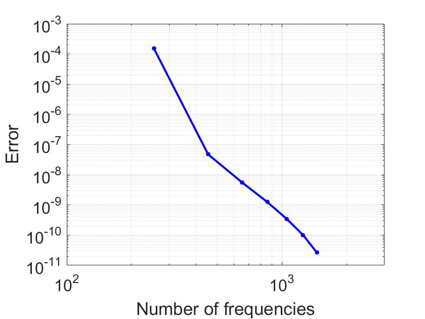
along the incident direction $d^{\textrm{inc}}=(1,0)$ with $t_{\textrm{lag}}=2$ . Together with a sufficiently fine fixed spatial discretization, the fixed numerical frequency intervals $\omega\in[5,25]$ and $\omega\in[-20,20]$ were used for the incident fields $u_{1}^{i}$ and $u_{2}^{i}$ , respectively. Figures 5 and 6 present the scattered field as a function of time $t$ at the observation point $x=(0.5,0)$ and the corresponding numerical errors at that point, respectively, as functions of the number of frequencies used—demonstrating the fast convergence of the algorithms as the frequency-domain discretization is refined.

Example 3. This example presents the solutions produced by the full hybrid ping-pong multiple scattering algorithm for the wave equation problem (2.1) in two different domains $\Omega$ , namely, the unit disc centered at the origin and the unit square $\Omega=[-1,1]^{2}$ , for $t\in[0,10]$ , and for each one of the two time-domain sources considered in Example 2: the point source $u_{1}^{i}(x,t)$ and the plane wave source $u_{2}^{i}(x,t)$ . For the plane-wave incidence case the exact solution is given by $u^{s}(x,t)=-u_{2}^{i}(x,t)$ for $x\in\Omega$ . In this example, the extensions $\widetilde{\Gamma}_{j}$ of $\Gamma_{j}$ for $j=1,2$ are constructed by means of portions of tangent circular arcs of radii $0.1$ . For the wave equation problem (2.1) in a unit disc domain, the numerical errors as a function of $M$ are displayed in Figures 7 and 8: clearly, rapid convergence and high accuracy are observed. Figures 9 and 10 display the total field within the rectangular domain $\Omega$ at various times, for two different point-source locations $z$ , and two different values of $\omega_{0}$ in (4.2), and using a total of $M=10$ ping-pong iterations; we have verified that, in this case, the numerical errors are less than $10^{-8}$ for all $t\in[0,10]$ .

Example 4. We now use Algorithm 4 to solve wave equation problems in a disc-shaped domain (Figure 1(c)) and a T-shaped domain (Figure 11(a)), up to final times $T=10$ , and using $M=7$ ping-pong iterations. The incident wave is a pulse function given by

u^{i}(x,t)=f(t-|x-z_{0}|/c),\quad f(s)=\sin(4s)e^{-1.6(s-3)^{2}},

(4.4)

which is displayed in Figure 11(b). Figure 11(c) displays the corresponding Fourier transform, in view of which the fixed numerical bandwidth value $W=15$ was used for this example. Figures 12-14 display the total field within $\Omega$ at various times and for different source point locations.

Example 5. This example concerns a long time propagation and scattering problem in a unit disc domain under the incident wave (4.4) with $z_{0}=(0,0)$ . For this example we have used $\delta_{12}=2\sin\frac{\pi}{10}\approx 0.618$ , $M=45$ , $K=4$ (so that $s_{K}+H=55$ ), $W=20$ , $J=454$ , and $\Delta t=0.11$ , and we have computed the necessary frequency domain solutions using open-arc discretizations $\mathcal{M}_{j},j=1,2$ , each one of which contains 224 discretization points. Note that the exact solution values at the points $x=(-\sqrt{3}/4,1/4)$ and $x=(0.5,0)$ coincide (since $|(-\sqrt{3}/4,1/4)|=|(0.5,0)|=0.5$ ). This simple symmetry relation provides a valuable verification of the numerical solution—which, as illustrated Figure 15, is closely satisfied by the numerical solution. Tables 2 and 3, finally, present the numerical solution errors $\max_{t\in[0,T(M)]}|u^{s}_{\rm num}-u^{s}_{\rm ref}|$ for the present problem at the point $x=(0.5,0)$ , for various values of $M$ and corresponding final times $T(M)$ , together with other statistics such as precomputation time and total computational times. Note in particular that the solution errors do not grow as the final times increase.

Table 2: Numerical errors, precomputation time and total computational times required by the problem considered in Example 5 for various values of

M

J=254

frequencies were used in all cases.

$M$	15	25	35	45
$T(M)$	8.652	14.832	21.012	27.192
Error	$6.57\times 10^{-4}$	$4.74\times 10^{-5}$	$1.87\times 10^{-5}$	$5.56\times 10^{-6}$
Time (precomputation)	9.1 s
Time ( $M$ iterations)	30.0 s	52.2 s	73.1 s	94.4 s

Table 3: Numerical errors, precomputation time and total computational times required by the problem considered in Example 5 for various values of

M

J=454

frequencies were used in all cases.

$M$	15	25	35	45
$T(M)$	8.652	14.832	21.012	27.192
Error	$1.24\times 10^{-7}$	$2.59\times 10^{-8}$	$1.10\times 10^{-8}$	$4.36\times 10^{-9}$
Time (precomputation)	16.8 s
Time ( $M$ iterations)	46.3 s	78.4 s	109.8 s	141.3 s

Example 6. In our final example we briefly demonstrate the feasibility of a version of the proposed multiple scattering algorithm which utilizes more than two patches. This extended algorithm requires use of appropriately windowed boundary data for the open-surface wave equation problems associated with multiple patches. At each step, the multiple wave equation problems can be solved in parallel. Complete details concerning the algorithm and its implementation will be presented elsewhere [12]. In the example presented here a three-patch decomposition of the boundary $\Gamma$ , as shown in Figure 16, is utilized to solve once again the wave equation problem (2.1) on the unit disc, under plane-wave incidence $u_{2}^{i}(x,t)$ , considered in Example 2, and the exact solution is given by $u^{s}(x,t)=-u_{2}^{i}(x,t)$ for $x\in\Omega$ . The numerical solutions at $x=(0.5,0)$ as functions of time $t$ for various values of $M$ are displayed in Figure 17. The maximum numerical errors are of the same order as those displayed in Figure 8(b) for the two-patch case.

5 Conclusions

This paper proposed a frequency-time hybrid integral-equation method for the wave equation problem in an interior two-dimensional bounded spatial domain. The solver is based on a novel ping-pong multiple scattering strategy that reduces the original problem to a sequence of problems of scattering by open-arcs. Exploiting the Huygens principle, relying on a domain decomposition strategy based on use of overlapping patches, and utilizing boundary integral equation formulations for frequency-domain sub-problems and an efficient Fourier transform algorithm, the proposed method produces the interior time-domain solution efficiently and with high accuracy. An extension of the ping-pong algorithm that incorporates arbitrary numbers of overlapping subdomains should enable application of the method to complex 2D and 3D geometries. The method can also be extended to enable solution of elastic and electromagnetic wave problems, and including problems of scattering by impenetrable obstacles, problems of transmission for penetrable structures and problems in multi-layered media. Such extensions, which lie beyond the scope of this paper, are left for future work.

Acknowledgments

OB gratefully acknowledges support from NSF, DARPA and AFOSR through contracts DMS-2109831, HR00111720035, FA9550-19-1-0173 and FA9550-21-1-0373, and by the NSSEFF Vannevar Bush Fellowship under contract number N00014-16-1-2808. TY gratefully acknowledges support from NSFC through Grants No. 12171465 and 12288201.

Appendix A Appendix

This appendix obtains the explicit expression (2.3), used in the proof of Lemma 2.4, for the solution $v_{+}^{s}(x,t)$ of problem (2.15), where $g$ is a causal function ( $g(x,t)=0$ for $t\leq 0$ ) defined on $\mathbb{R}_{0}^{2}\times\mathbb{R}$ , which satisfies the assumption (2.13) for a bounded subset $\mathcal{C}^{\mathrm{inc}}\subset\mathbb{R}_{0}^{2}$ . The construction utilizes the associated frequency-domain Green’s function $G_{\omega}(x,y)$ , which, for each $y\in{\mathbb{R}}^{2}_{+}$ , is defined as the solution of the problem

\displaystyle\begin{cases}\Delta_{x}G_{\omega}(x,y)+\kappa^{2}G_{\omega}(x,y)=-\delta_{y}(x),&(x,\omega)\in{\mathbb{R}}^{2}_{+}\times{\mathbb{R}},\ \kappa=\omega/c,\cr G_{\omega}(x,y)=0&(x,\omega)\in{\mathbb{R}}_{0}\times{\mathbb{R}}.\end{cases}

As is well known, the method of images yields

\displaystyle G_{\omega}(x,y)=\frac{i}{4}H_{0}^{(1)}(\kappa|x-y|)-\frac{i}{4}H_{0}^{(1)}(\kappa|x^{\prime}-y|),\quad x\neq y,

(A.1)

where $x^{\prime}=(x_{1},-x_{2})$ denotes the image point of $x=(x_{1},x_{2})\in{\mathbb{R}}^{2}_{+}$ with respect to ${\mathbb{R}}^{2}_{0}$ , and where $H_{0}^{(1)}$ denotes the Hankel function of first kind and order zero. Let now $V_{+}^{s}(x,\omega)$ denote the Fourier transform of $v_{+}^{s}(x,t)$ with respect to $t$ for $x\in{\mathbb{R}}^{2}_{+}$ ; clearly $V_{+}^{s}$ is a solution of the Helmholtz equation with wavenumber $\kappa$ in ${\mathbb{R}}^{2}_{+}$ , and with Dirichlet boundary conditions $V_{+}^{s}=\widehat{g}$ on ${\mathbb{R}}^{2}_{0}$ —where $\widehat{g}(x,\omega)$ denotes the Fourier transform of $g(x,t)$ with respect to $t$ . Clearly $\widehat{g}(x,\omega)$ vanishes for $x\not\in\mathcal{C}^{\mathrm{inc}}$ since, in view of (2.13), so does $g(x,t)$ . Use of Green’s theorem together with the Green function $G_{\omega}$ [30] yields

\displaystyle V_{+}^{s}(x,\omega)=\int_{\mathcal{C}^{\mathrm{inc}}}\partial_{\nu_{y}}G_{\omega}(x,y)\widehat{g}(y,\omega)ds_{y},\quad x\in{\mathbb{R}}^{2}_{+},

(A.2)

where, denoting by $\nu_{y}=(0,1)^{\top}$ the unit upward normal on ${\mathbb{R}}^{2}_{0}$ ,

\displaystyle{\color[rgb]{0,0,0}\partial_{\nu_{y}}G_{\omega}(x,y)=\frac{i\kappa}{2}\frac{x_{2}}{|x-y|}H_{1}^{(1)}(\kappa|x-y|).}

It follows that, for $x\in{\mathbb{R}}^{2}_{+}$ , $v_{+}^{s}(x,t)$ equals the inverse Fourier transform of (A.2). To proceed with the construction we introduce the following notations. We call ${\mathbb{R}}^{3}_{0}={\mathbb{R}}^{2}_{0}\times{\mathbb{R}}$ the plane in three dimensional space with cross-section ${\mathbb{R}}^{2}_{0}$ , we let $\breve{x}=(x^{\top},0)^{\top}\notin{\mathbb{R}}^{3}_{0}$ , $\breve{y}=(y^{\top},z)^{\top}\in{\mathbb{R}}^{3}_{0}$ and $\breve{r}=\sqrt{r^{2}+z^{2}}$ with $r=|x-y|=\sqrt{(x_{1}-y_{1})^{2}+(x_{2}-y_{2})^{2}}$ . Using the unit normal $\nu_{y}=(0,1)^{\top}$ of ${\mathbb{R}}^{2}_{0}$ , finally, the corresponding unit normal on ${\mathbb{R}}^{3}_{0}$ is denoted by $\nu_{\breve{y}}=(0,1,0)^{\top}$ .

In preparation for the main result of this appendix we establish the following Lemma.

Lemma A.1.

The following formulas hold:

	$\displaystyle\frac{1}{4\pi}\int_{-\infty}^{\infty}\frac{e^{i\kappa\breve{r}}}{\breve{r}}dz=\frac{i}{4}H_{0}^{(1)}(\kappa r),$		(A.3)
	$\displaystyle\frac{1}{4\pi}\int_{-\infty}^{\infty}\partial_{y_{i}}\left(\frac{e^{i\kappa\breve{r}}}{\breve{r}}\right)dz=\frac{i}{4}\partial_{y_{i}}H_{0}^{(1)}(\kappa r),\quad i=1,2.$		(A.4)

Proof.

The expression (A.3) is established in [27, Lemma 3.1]. Using the notations

\displaystyle\breve{r}_{0}=(x_{1}^{2}+(x_{2}-y_{2})^{2}+z^{2})^{1/2},

to establish the $y_{1}$ component of (A.4) (the $y_{2}$ component follows analogously), it suffices to show that

\displaystyle\int_{0}^{y_{1}}dy_{1}\int_{1}^{\infty}\partial_{y_{1}}\left(\frac{e^{i\kappa\breve{r}}}{\breve{r}}\right)dz=\int_{1}^{\infty}\frac{e^{i\kappa\breve{r}}}{\breve{r}}dz-\int_{1}^{\infty}\frac{e^{i\kappa\breve{r}_{0}}}{\breve{r}_{0}}dz;

(A.5)

the result then follows by differentiation with respect to $y_{1}$ . To establish (A.5), we seek to utilize Fubini’s Theorem on the left hand integral, but, unfortunately, the integrand does not satisfy the hypothesis of Fubini’s theorem: it is not an integrable function of the variable $(y_{1},z)$ . To address this difficulty we integrate by parts the left-hand integral: using the relation

\displaystyle e^{i\kappa\breve{r}}=\frac{\breve{r}}{i\kappa z}\partial_{z}e^{i\kappa\breve{r}},

(A.6)

we obtain

\displaystyle\int_{1}^{\infty}\partial_{y_{1}}\left(\frac{e^{i\kappa\breve{r}}}{\breve{r}}\right)dz=\int_{1}^{\infty}\frac{1}{i\kappa z}\partial_{z}\partial_{y_{1}}e^{i\kappa\breve{r}}dz=-\frac{1}{i\kappa}\partial_{y_{1}}e^{i\kappa\breve{r}}\Big|_{z=1}+\int_{1}^{\infty}\frac{1}{i\kappa z^{2}}\partial_{y_{1}}e^{i\kappa\breve{r}}dz.

Fubini’s Theorem can now be applied to the last integral, and we thus obtain

	$\displaystyle\int_{0}^{y_{1}}dy_{1}\int_{1}^{\infty}\partial_{y_{1}}\left(\frac{e^{i\kappa\breve{r}}}{\breve{r}}\right)dz$	$\displaystyle=$	$\displaystyle-\frac{1}{i\kappa}e^{i\kappa\breve{r}}\Big\|_{z=1}+\frac{1}{i\kappa}e^{i\kappa\breve{r}_{0}}\Big\|_{z=1}+\int_{0}^{y_{1}}dy_{1}\int_{1}^{\infty}\frac{1}{i\kappa z^{2}}\partial_{y_{1}}e^{i\kappa\breve{r}}dz$
		$\displaystyle=$	$\displaystyle-\frac{1}{i\kappa}e^{i\kappa\breve{r}}\Big\|_{z=1}+\frac{1}{i\kappa}e^{i\kappa\breve{r}_{0}}\Big\|_{z=1}+\int_{1}^{\infty}\frac{1}{i\kappa z^{2}}(e^{i\kappa\breve{r}}-e^{i\kappa\breve{r}_{0}})dz.$

Now, replacing $z^{-2}=-\partial_{z}z^{-1}$ and integrating by parts in the last integral, and then using (A.6) once again, equation (A.5) results, as desired. The proof is now complete. ∎

To establish (2.3) we proceed as follows. In view of Lemma A.1 and equation (A.1), and noting that for $x\in{\mathbb{R}}^{2}_{+},y\in{\mathbb{R}}^{2}_{0}$ we have $x_{2}-y_{2}\neq 0$ , the normal derivative of the Green function on the boundary ${\mathbb{R}}^{2}_{0}$ is given by

\displaystyle\partial_{\nu_{y}}G_{\omega}(x,y)

\displaystyle=

\displaystyle\frac{i\kappa}{2}\frac{x_{2}}{r}H_{1}^{(1)}(\kappa r)=\frac{i}{2}\partial_{y_{2}}H_{0}^{(1)}(\kappa r)=\frac{1}{2\pi}\int_{-\infty}^{\infty}\partial_{y_{2}}\left(\frac{e^{i\kappa\breve{r}}}{\breve{r}}\right)dz=-\frac{1}{2\pi}\int_{-\infty}^{\infty}\frac{i\kappa\breve{r}-1}{\breve{r}^{3}}x_{2}e^{i\kappa\breve{r}}dz

and, therefore, equation (A.2) gives

\displaystyle V_{+}^{s}(x,\omega)=-\frac{1}{2\pi}\int_{\mathcal{C}^{\mathrm{inc}}\times{\mathbb{R}}}\frac{i\kappa\breve{r}-1}{\breve{r}^{3}}x_{2}e^{i\kappa\breve{r}}\,\widehat{g}(y,\omega)ds_{\breve{y}},\quad x\in{\mathbb{R}}^{2}_{+}.

Taking the inverse Fourier transform we obtain

	$\displaystyle v_{+}^{s}(x,t)$	$\displaystyle=$	$\displaystyle\frac{1}{2\pi}\int_{\mathcal{C}^{\mathrm{inc}}\times{\mathbb{R}}}\int_{0}^{t}\left[\frac{1}{\breve{r}^{3}}\delta(t-\tau-c^{-1}\breve{r})+\frac{1}{c\breve{r}^{2}}\delta^{\prime}(t-\tau-c^{-1}\breve{r})\right]x_{2}\,g(y,\tau)d\tau ds_{\breve{y}}$
		$\displaystyle=$	$\displaystyle\frac{1}{2\pi}\int_{\mathcal{C}^{\mathrm{inc}}\times{\mathbb{R}}}\left[\frac{1}{\breve{r}^{3}}g(y,t-c^{-1}\breve{r})+\frac{1}{c\breve{r}^{2}}g^{(1)}(y,t-c^{-1}\breve{r})\right]x_{2}ds_{\breve{y}}.$

where $g^{(1)}(x,t)=\frac{\partial g}{\partial t}(x,t)$ . Using the relations $ds_{\breve{y}}=dzds_{y}$ we thus obtain

	$\displaystyle v_{+}^{s}(x,t)$	$\displaystyle=$	$\displaystyle\frac{1}{\pi}\int_{\mathcal{C}^{\mathrm{inc}}}\int_{0}^{+\infty}\Big[(r^{2}+z^{2})^{-3/2}g(y,t-c^{-1}\sqrt{r^{2}+z^{2}})$
			$\displaystyle\quad\quad\quad+\frac{1}{c(r^{2}+z^{2})}g^{(1)}(y,t-c^{-1}\sqrt{r^{2}+z^{2}})\Big]x_{2}dzds_{y}.$

Utilizing the change of variables $\tau=t-c^{-1}\sqrt{r^{2}+z^{2}}$ , or equivalently $z=c\sqrt{(t-\tau)^{2}-c^{-2}r^{2}}$ , and $dz=-cz^{-1}\sqrt{r^{2}+z^{2}}d\tau$ , we then obtain

\displaystyle(r^{2}+z^{2})^{-3/2}dz=-\frac{1}{c^{2}(t-\tau)^{2}\sqrt{(t-\tau)^{2}-c^{-2}r^{2}}}d\tau

and

\displaystyle\frac{1}{c(r^{2}+z^{2})}dz=-\frac{1}{c^{2}(t-\tau)\sqrt{(t-\tau)^{2}-c^{-2}r^{2}}}d\tau.

It then follows that, for $x\in{\mathbb{R}}^{2}_{+}$ ,

	$\displaystyle v_{+}^{s}$	$\displaystyle(x,t)=\frac{1}{\pi c^{2}}$		(A.7)
		$\displaystyle\int_{\mathcal{C}^{\mathrm{inc}}}\int_{0}^{t-c^{-1}\|x-y\|}\left[\frac{x_{2}\,g(y,\tau)}{(t-\tau)^{2}\sqrt{(t-\tau)^{2}-c^{-2}\|x-y\|^{2}}}+\frac{x_{2}\,g^{(1)}(y,\tau)}{(t-\tau)\sqrt{(t-\tau)^{2}-c^{-2}\|x-y\|^{2}}}\right]d\tau ds_{y},$		(A.8)

as desired.

Remark A.2.

Although not used in this paper, it is worthwhile to note here that, for an arbitrary two-dimensional Lipschitz curve $\Gamma$ , and letting $\breve{\Gamma}=\Gamma\times{\mathbb{R}}$ , the changes of variables used in this appendix can easily be utilized to obtain an expression for the time-domain double-layer potential in two-dimensions, which had heretofore not been successfully derived. Utilizing once again the notations used above, from the Kirchhoff formula [55, Eq. (22), Sec. 8.1], we know that the classical three-dimensional time-domain double-layer potential is given by

\displaystyle\mathcal{D}_{3D}(\phi)(\breve{x},t)=\frac{1}{4\pi}\int_{\breve{\Gamma}}\left[\frac{\partial(\breve{r}^{-1})}{\partial\nu_{\breve{y}}}\phi(\breve{y},t-c^{-1}\breve{r})-\frac{1}{c\breve{r}}\frac{\partial\breve{r}}{\partial\nu_{\breve{y}}}\phi^{(1)}(\breve{y},t-c^{-1}\breve{r})\right]ds_{\breve{y}}.

The two-dimensional double-layer potential $\mathcal{D}_{2D}$ can then be obtained by assuming that the causal signal $\phi$ is independent of $z$ . Then using the change of variables $\tau=t-c^{-1}\sqrt{r^{2}+z^{2}}$ we obtain

	$\displaystyle\mathcal{D}_{2D}(\phi)(x,t)$
	$\displaystyle=\frac{1}{2\pi c^{2}}\int_{\Gamma}\int_{0}^{t-c^{-1}\|x-y\|}\left[\frac{(x-y)\cdot\nu_{y}\phi(y,\tau)}{(t-\tau)^{2}\sqrt{(t-\tau)^{2}-c^{-2}\|x-y\|^{2}}}+\frac{(x-y)\cdot\nu_{y}\phi^{(1)}(y,\tau)}{(t-\tau)\sqrt{(t-\tau)^{2}-c^{-2}\|x-y\|^{2}}}\right]d\tau ds_{y}.$

which provides a correction to the expression presented in [51, Page 19]. The contributions [8, Sections 6.3-6.5], [38, Page 42] and references therein outline some of the difficulties previously encountered in regard to the 2D double-layer potential.

References

[1] A. Aimi, M. Diligenti, C. Guardasoni, On the energetic Galerkin boundary element method applied to interior wave propagation problems, J. Comput. Appl. Math. 235(7) (2011) 1746-1754.
[2] B. Alpert, L. Greengard, T. Hagstrom, Nonreflecting boundary conditions for the time-dependent wave equation, J. Comput. Phys. 180 (2002) 270-296.
[3] F. Amlani, O.P. Bruno, An FC-based spectral solver for elastodynamic problems in general three-dimensional domains, J. Comput. Phys. 307 (2016) 333-354.
[4] K.E. Atkinson, I.H. Sloan. The numerical solution of first-kind logarithmic-kernel integral equations on smooth open arcs. Math. Comp. 56 (1991) 119-139.
[5] T.G. Anderson, Hybrid Frequency-Time Analysis and Numerical Methods for Time-Dependent Wave Propagation (Ph.D. thesis), California Institute of Technology, 2020.
[6] T.G. Anderson, O.P. Bruno, M. Lyon, High-order, dispersionless “fast-hybrid” wave equation solver. Part I: O(1) sampling cost via incident-field windowing and recentering, SIAM J. Sci. Comput. 422 (2020) A1348-A1379.
[7] I.M. Babuška, S.A. Sauter, Is the pollution effect of the FEM avoidable for the Helmholtz equation considering high wave numbers? SIAM J. Numer. Anal. 34 (1997) 2392-2423.
[8] B.B. Baker, E.T. Copson, The Mathematical Theorey Huygens’ Principle, Oxford at the Clarendon Press, 1939.
[9] A. Bamberger, T. Ha-Duong, Formulation variationelle espace-temps pour le calcul par potentiel retardé de la diffraction d’une onde acoustique, Math. Methods Appl. Sci. 8 (1986) 405-435.
[10] L. Banjai, M. Kachanovska, Fast convolution quadrature for the wave equation in three dimensions, J. Comput. Phy. 279 (2014) 103-126.
[11] P. Bansal, A. Moiola, I. Perugia, C. Schwab, Space-time discontinuous Galerkin approximation of acoustic waves with point singularities, IMA J. Numer. Anal. 41 (2021) 2056-2109.
[12] G. Bao, O.P. Bruno, T. Yin, Multiple-scattering frequency-time hybrid integral equation solver for the wave equation problems with bounded obstacles, in preparation.
[13] A.H. Barnett, L. Greengard, T. Hagstrom, High-order discretization of a stable time-domain integral equation for 3D acoustic scattering, J. Comput. Phy. 402 (2020) 109047.
[14] C. Bauinger, O.P. Bruno, “Interpolated Factored Green Function” method for accelerated solution of scattering problems, J. Comput. Phy. 430 (2021) 110095.
[15] J.-P. Berenger, A perfectly matched layer for the absorption of electromagnetic waves, J. Comput. Phy. 114 (1994) 185-200.
[16] T. Betcke, N. Salles, and W. Śmigaj, Overresolving in the laplace domain for convolution quadrature methods, SIAM J. Sci. Comput. 39 (2017), pp. A188–A213.
[17] O.P. Bruno, M. Lyon, C. Pérez-Arancibia, C. Turc, Windowed Green function method for layered-media scattering, SIAM J. Appl. Math. 76(5) (2016) 1871-1898.
[18] O.P. Bruno, E. Garza, A Chebyshev-based rectangular-polar integral solver for scattering by general geometries described by non-overlapping patches, J. Comput. Phys. 421 (2020) 109740.
[19] O.P. Bruno, E. Garza, C. Pérez-Arancibia, Windowed Green function method for nonuniform open-waveguide problems, IEEE Trans. Antenn. Propag. 65 (2017) 4684-4692.
[20] O.P. Bruno, S. Lintner, A high-order integral solver for scalar problems of diffraction by screens and apertures in three-dimensional space, J. Comput. Phys. 252 (2013).
[21] O.P. Bruno, S. Lintner, Second-kind integral solvers for TE and TM problems of diffraction by open arcs, Radio Sci. 47 (6) (2012).
[22] O.P. Bruno, L. Kunyansky, A fast, high-order algorithm for the solution of surface scattering problems: Basic implementation, tests, and applications, J. Comput. Phys. 169 1 (2001) 80-110.
[23] O.P. Bruno, M. Lyon, High-order unconditionally stable FC-AD solvers for general smooth domains I. Basic elements, J. Comput. Phys. 229 (6) (2010) 2009-2033.
[24] O.P. Bruno, T. Yin, Regularized integral equation methods for the elastic scattering problems in three dimensions, J. Comput. Phys. 410 (2020) 109350.
[25] O.P. Bruno, T. Yin, A windowed Green function method for elastic scattering problems on a half-space, Comput. Methods Appl. Mech. Engrg. 376 (2021) 113651.
[26] Q. Chen, H. Haddar, A. Lechleiter, P. Monk, A sampling method for inverse scattering in the time domain, Inverse Problems 8 (2010) 85001-85017.
[27] X. Chen, A. Friedman, Maxwell’s equations in a periodic structure, Transactions of the American Mathematical Society 323 (1991) 465-507.
[28] D. Colton and R. Kress, Inverse Acoustic and Electromagnetic Scattering Theory, Berlin, Springer, 1998.
[29] M. Costabel, M. Dauge, R. Duduchava, Asymptotics without logarithmic terms for crack problems, Commun. Partial Differ. Equ. 28 (2003) 869-926.
[30] J. DeSanto, P.A. Martin, On the derivation of boundary integral equations for scattering by an infinite one-dimensional rough surface, J. Acous. Soc. Am. 102(1) (1997) 67-77.
[31] J. Douglas, J.E. Santos, D. Sheen, L.S. Bennethum, Frequency domain treatment of one-dimensional scalar waves, Math. Models Methods Appl. Sci. 3 (1993) 171-194.
[32] T. Ha-Duong, On retarded potential boundary integral equations and their discretisation, in Topics in Computational Wave Propagation: Direct and Inverse Problems, M. Ainsworth et al., eds., Springer Berlin Heidelberg, Berlin, Heidelberg, 2003, pp. 301–336.
[33] B. Engquist, A. Majda, Absorbing boundary conditions for the numerical simulation of waves, Math. Comp. 31 (1977) 629–629.
[34] L.C. Evans, Partial Differential Equations (2nd edition), Graduate Studies in Mathematics, Vol. 19, American Mathematical Society, Providence, 2010.
[35] D.A. French, T.E. Peterson, A continuous space-time finite element method for the wave equation, Math. Comp. 65 (1996) 491-506.
[36] M.J. Grote, A. Schneebeli, D. Schötzau, Dicontinuous Galerkin finite element method for the wave equation, SIAM J. Numer. Anal. 44 (2006) 2408-2431.
[37] M. Hassell, T. Qiu, T. Sánchez-Vizuet, F.-J. Sayas, A new and improved analysis of the time domain boundary integral operators for acoustics, J. Integral Equations Applications 29(1) (2017) 107-136.
[38] D.S. Jones, The Theory of Electromagnetism, Pergamon Press Oxford, 1964.
[39] I. Labarca, R. Hiptmair, Acoustic scattering problems with convolution quadrature and the method of fundamental solutions, Commun. Comput. Phys. 30 (2021) 985-1008.
[40] A.R. Laliena, F.-J. Sayas, Theoretical aspects of the application of convolution quadrature to scattering of acoustic waves, Numer. Math. 112 (2009) 637-678.
[41] J.-F. Lee, R. Lee, A. Cangellaris, Time-domain finite-element methods, IEEE Trans. Antenn. Propag. 45 (1997) 430–442.
[42] Y. Li, W. Zheng, X. Zhu, A CIP-FEM for high-frequency scattering problem with the truncated DtN boundary condition, CSIAM Trans. Appl. Math. 1(3) (2020) 530-560.
[43] S. Lintner, O.P. Bruno, A generalized Calderón formula for open-arc diffraction problems: theoretical considerations, Proceedings of the Royal Society of Edinburgh Section A: Mathematics 145(2) (2015) 331-364.
[44] Y. Liu, Fast Multipole Boundary Element Method, Cambridge University Press, New York, 2009.
[45] R. Löscher, O. Steinbach, M. Zank, Numerical results for an unconditionally stable space-time finite element method for the wave equation, arXiv:2103.04324.
[46] C. Lubich, On the multistep time discretization of linear initial-boundary value problems and their boundary integral equations, Numer. Math. 67 (1994) 365-389.
[47] R. C. MacCamy, Low frequency acoustic oscillations, Q. Appl. Math. 23 (1965) 247-255.
[48] E. Mecocci, L. Misici, M. C. Recchioni, F. Zirilli, A new formalism for time-dependent wave scattering from a bounded obstacle, J. Acoust. Soc. Am. 107 (2000) 1825-1840.
[49] J. Nečas, Direct Methods in the Theory of Elliptic Equations, Springer, 2012.
[50] T.v. Petersdorff, E.P. Stephan, A direct boundary element method for interface crack problems, In: S.N. Atluri, G. Yagawa (eds), Computational Mechanics ’88, 1988, pp. 329-333, Springer.
[51] F.-J. Sayas, Retarded Potentials and Time Domain Boundary Integral Equations, Springer International Publishing, 2016.
[52] O. Steinbach, C. Urzúa-Torres, A new approach to space-time boundary integral equations for the wave equation, SIAM J. Math. Anal. 54(2) (2022) 1370-1392.
[53] O. Steinbach, C. Urzúa-Torres, M. Zank, Towards coercive boundary element methods for the wave equation, arXiv:2106.01646.
[54] E.P. Stephan, W.L. Wendland, An augmented Galerkin procedure for the boundary integral method applied to two-dimensional screen and crack problems, Appl. Anal. 3 (1984) 183-219.
[55] J.A. Stratton, Electromagnetic theory, McGraw-Hill, New York, 1941.
[56] A. Taflove, Computational electrodynamics: the finite-difference time-domain method, Artech House, Boston, 2000.
[57] P. Werner, Low frequency asymptotics for the reduced wave equation in two-dimensional exterior spaces, Math. Meth. Appl. Sci. 8 (1986): 134-156.
[58] Y. Xing, C.-S. Chou, C.-W. Shu, Energy conserving local discontinuous Galerkin methods for wave propagation problems, Inverse Probl. Imag. 7 (2013) 967-986.
[59] A. Yilmaz, J.-M. Jin, E. Michielssen, Time domain adaptive integral method for surface integral equations, IEEE Trans. Antenn. Propag., 52 (2004), 2692-2708.
[60] X. Yuan, G. Bao, P. Li, An adaptive finite element DtN method for the open cavity scattering problems, CSIAM Trans. Appl. Math. 12 (2020) 316-345.
[61] Y. Yue, F. Ma, B. Chen, Time domain linear sampling method for inverse scattering problems with cracks, E. Asian J. Appl. Math. 12(1) (2022) 96-110.


(a) $t=3$	(b) $t=5$

(c) $t=7$	(d) $t=9$


(a) $t=3$	(b) $t=5$

(c) $t=7$	(d) $t=9$


(a) T-shaped domain.	(b) $u^{i}(x,t)$ for $\|x-z_{0}\|=1.$	(c) $U^{i}(x,\omega).$