Estimation and variable selection in joint mean and dispersion models applied to mixture experiments

Experiments with mixtures involve the mixing or blending of two or more ingredients to form an end product. For this type of experiment is of interest to determine the proportions of the mixture components which lead to desirable results with respect to some quality characteristic of interest. An excellent introduction to mixture experiments, including a chronological sequence of papers that appeared in the statistical literature in this area from 1953 to 2009, is given by Cornell 2011.

Classical regression models are usually used in mixture experiments, which assume normality of errors, constant variance and linearity of systematic effects. However, situations may arise where such assumptions cannot be completely satisfied. According to Nelder and Lee 1991, for many data sets the assumptions underlying classical linear models are unsatisfactory and transformations of response variable cannot necessarily satisfy all three criteria including the normality.

Generalized linear models (GLMs) allow the analysis of data for which the assumptions of the classical regression model are not satisfied and provide a general framework for modeling variability through joint modeling of mean and dispersion (JMMD) that allows joint models to be build for the mean and dispersion. The JMMD was introduced by Nelder and Lee 1991 as an alternative to Taguchi’s methods in quality-improvement experiment and provides a methodology to find and check the fit of the models found with a solid statistical basis. Further examples of applications appeared in Lee and Nelder 1998 and Lee and Nelder 2003. In generalized linear models, the response variance is equal to the dispersion parameter multiplied by a function of the mean, called the variance function. Only in the case of normal distribution, where the variance function is the identity function, the dispersion parameter coincides with the variance of the response, see McCullagh and Nelder 1989 for more details.

In mixture experiments, modeling of variance is only considered in situations where noise variables exist. Noise variables or uncontrollable variables are process variables that vary naturally and uncontrollably during the production but may be controlled during the experiment, such as humidity or temperature, see Montgomery 2017. p. 571. Process variables are factors in an experiment that do not form any portion of the mixture but whose levels when changed could affect the blending properties of the ingredients, see, for example, Cornell 2011, p. 247, for more details.

Statistical modeling of variance in mixture experiments with noise variables has been considered in Steiner and Hamada 1997, who proposed a combined mixture-process-noise variable model, built and solved an optimization problem to minimize a quadratic loss function, taking into account both the mean and variance of response. Another approach to modeling the variance in mixture experiments with noise variables is due to Goldfarb et al. 2003 using the delta method, which employs a first-order Taylor series approximation of the regression model at a vector of noise variables. The delta method is a well-known technique, based on Taylor series expansions, for finding approximations to the mean and variance of functions of random variables. For a comprehensive treatment of the delta method, see Casella and Berger 2002, p. 240. An application of the delta method for modeling variability in mixture experiments with noise variables in food engineering is also presented in Granato et al. 2020. However, in all approaches presented for modeling the variance, normality of errors and constant dispersion parameter were considered. Thus, the mean model was considered normal homoscedastic and the modeling of variance was due only to noise variables.

The approach we consider is quite general because, when considering the class of generalized linear models, distributions other than the normal distribution may be considered. In addition, considering a dispersion model, the variability modeling process allows modeling the variance not only in situations where noise variables exist.

The purpose of this article is to show how joint modeling of mean and dispersion can be applied to model the variability in mixture experiments. We give a comprehensive understanding of the parameter estimation process in JMMD and we propose a procedure of variable selection adapted to the conditions of the mixture experiments. A simulation study was used to exemplify the proposed variable selection procedure. The considered methodology was applied to an example from the Food Industry, where a detailed explanation of the proposed method was presented.

The paper is organized as follows. In Section 2, we introduce the mixture experiments. In Section 3, we provide a summary of the joint modeling of mean and dispersion, discussing the principal points of the theory. A variable selection process, adapted to mixture experiments, is also presented. A simulation study, considering Normal distribution for the response variable, is shown in Section 4. In Section 5, we show how the joint modeling of mean and dispersion can be applied to a practical bread-making problem involving three mixture ingredients, three types of flour, and subject to two noise variables, mixing time and proofing time for the dough. Final considerations are given in Section 6.

A mixture experiment involves mixing proportions of two or more components to make different compositions of an end product. In mixture experiments, the main aim is at determining the proportions of the mixture components which lead to desirable properties of the response variable. Mixture component proportions $x_{i}$ are subject to the constraints

In consonance with Khuri 2005, consider the standard model in a mixture experiment the linear model $\mbox{\boldmath{$Y$}}=\mbox{\boldmath{$X$}}\mbox{\boldmath{$\beta$}}+\mbox{\boldmath{$\epsilon$}}$, where $\mbox{\boldmath{$Y$}}^{t}=(Y_{1},\ldots,Y_{n})$ is a response vector, $X$ is a known design matrix of order $n\times n_{p}$ and rank $n_{p}\leq n$, $\mbox{\boldmath{$\beta$}}^{t}=(\beta_{1},\ldots,\beta_{n_{p}})$ is an unknown parameter vector, and $\mbox{\boldmath{$\epsilon$}}^{t}=(\epsilon_{1},\ldots\epsilon_{n})$ is a random error vector with a zero mean and a variance-covariance matrix $\sigma^{2}\mbox{\boldmath{$I$}}$, with $\sigma^{2}=Var(\epsilon_{i})$, for $i=1,\ldots,n$, and $I$ is the is the identity matrix of order $n$. The response value at any point $\mbox{\boldmath{$x$}}^{t}=(x_{1},\ldots,x_{a})$ in a region of interest $\cal{R}$ is given by $Y(\mbox{\boldmath{$x$}})=\zeta(\mbox{\boldmath{$x$}},\mbox{\boldmath{$\beta$}})+\epsilon$, where the linear predictor $\zeta(\mbox{\boldmath{$x$}},\mbox{\boldmath{$\beta$}})=\mbox{\boldmath{$f$}}^{t}(\mbox{\boldmath{$x$}})\mbox{\boldmath{$\beta$}}$ is a polynomial function of a certain degree in $x_{1},\ldots,x_{a}$. The vector $\mbox{\boldmath{$f$}}^{t}\left(\mbox{\boldmath{$x$}})=(f_{1}(\mbox{\boldmath{$x$}}),\ldots,f_{n_{p}}(\mbox{\boldmath{$x$}})\right)$ is of the same form as a row of $X$, but is evaluated at the point $x$. We can see that the linear predictor $\zeta(\mbox{\boldmath{$x$}},\mbox{\boldmath{$\beta$}})=E(Y(\mbox{\boldmath{$x$}}))$.

Models commonly used in experiments with mixture are the so-called Scheffé’s models. Scheffé 1958 proposed canonical polynomial models for mixture experiments, considering a reparametrization of the polynomial regression model, based on the mixture constraint in equation (2.1). For a comprehensive understanding of Scheffé’s models, see Cornell 2002 or Cornell 2011. The linear predictor of Scheffé’s first-order polynomial model is given by

For higher order models, the reparametrization does not lead to simple models; for example, for the third order model (cubic model), the linear predictor of Scheffé’s canonical polynomial model is given by

For estimation of model parameters, Scheffé proposed the simplex-lattice designs ($a,m$), which are characterized by symmetrical arrangements of points within the experimental region, where $m$ is the number of equally spaced parts in the interval $(0,1)$. The number of parameters in the canonical polynomial model is exactly equal to the number of points chosen within the experimental region. The simplex-lattice design ($a,m$) consists of $\frac{(a+m-1)!}{m!(a-1)!}$ experimental points. Each component of the mixture takes $m+1$ values equally spaced between 0 and 1, that is, $x_{i}=0,\frac{1}{m},\frac{2}{m},\ldots,\frac{m}{m}=1$ for $i=1,\ldots,a$. All mixtures involving these proportions are used in the experimental design. For more details on simplex-lattice designs, see Cornell 2002.

Alternatively to the Scheffé’s canonical models, we can also use models of mixture with slack variable. Due to the mixture restrictions (2.1), the proportions of the components are not independent; thus, knowing the proportions of the first $a-1$ components we can determine the proportion of the remaining component. In this way, the mixture models with slack variable can be obtained from the Scheffé’s canonical models by replacing the slack variable chosen, say $x_{l}$, by $1-\sum_{i\not=l}^{a}x_{i}$. The purpose of this process is to produce mixture models that depend on $a-1$ independent variables. For example, by defining $x_{a}$ as the slack variable, the linear predictor for the mixture model with slack variable obtained from Scheffé’s quadratic model (2.3) is given by

Note that, by comparing the coefficients of models (2.3) and (2.5), we have the following equivalences $\alpha_{0}=\beta_{a}$, $\alpha_{i}=\beta_{i}-\beta_{a}+\beta_{ia}$, $\alpha_{ii}=-\beta_{ia}$ and $\alpha_{ij}=\beta_{ij}-(\beta_{ia}+\beta_{ja})$, with $i=1,\ldots,a-1$ and $j=2,\ldots,a-1$.

The use of models with slack variable as well as the choice of which component should be designated as a slack variable is not clearly presented in the literature. Cornell 2011 highlights that the choice of which of the $a$ components to designate as the slack variable has not been defended from either a theoretical or a practical point of view. A discussion of the pros and cons of using slack variable is given by Cornell 2000; see also Smith 2005. Comparative studies between models of mixtures with slack variable and Scheffé’s models are given in Cornell 2002, Cornell and Gorman 2003 and Khuri 2005.

When in a mixture experiment, the response depends not only on the proportion of the mixture components, but also on the processing conditions, such as temperature, humidity or heating time, we have a mixture experiment with process variables. Problems of mixture experiments with process variables arise when in the mixture experiment the property of interest is a function of the proportions of the ingredients and of other factors that do not form any portion of the mixture. These factors, which depend on process conditions, are called process variables, see Cornell 2002, p. 354.

Usually, in problems of mixture experiments including process variables, the goal is determining the proportions of the mixture components along with situations of process conditions, in order to achieve an optimal or desirable property on the response variable.

Thus, if in addition to the $a$ mixture components $\mbox{\boldmath{$x$}}^{t}=(x_{1},\dots,x_{a})$ there are $r$ process variables $\mbox{\boldmath{$z$}}^{t}=(z_{1},\dots,z_{r})$, we can consider additive models like $\eta(\mbox{\boldmath{$x$}},\mbox{\boldmath{$z$}},\mbox{\boldmath{$\beta$}},\mbox{\boldmath{$\gamma$}})=\zeta(\mbox{\boldmath{$x$}},\mbox{\boldmath{$\beta$}})+\vartheta(\mbox{\boldmath{$z$}},\mbox{\boldmath{$\gamma$}})$ or complete cross product models of the type $\eta(\mbox{\boldmath{$x$}},\mbox{\boldmath{$z$}},\mbox{\boldmath{$\beta$}},\mbox{\boldmath{$\gamma$}})=\zeta(\mbox{\boldmath{$x$}},\mbox{\boldmath{$\beta$}})\vartheta(\mbox{\boldmath{$z$}},\mbox{\boldmath{$\gamma$}})$ or combinations of these such as $\eta(\mbox{\boldmath{$x$}},\mbox{\boldmath{$z$}},\mbox{\boldmath{$\beta$}},\mbox{\boldmath{$\gamma$}})=\zeta(\mbox{\boldmath{$x$}},\mbox{\boldmath{$\beta$}})+\nu(\mbox{\boldmath{$x$}},\mbox{\boldmath{$z$}},\mbox{\boldmath{$\beta$}},\mbox{\boldmath{$\gamma$}})$, where $\vartheta(\mbox{\boldmath{$z$}},\mbox{\boldmath{$\gamma$}})$ represents the linear predictor for the process variable model and $\nu(\mbox{\boldmath{$x$}},\mbox{\boldmath{$z$}},\mbox{\boldmath{$\beta$}},\mbox{\boldmath{$\gamma$}})$ comprises products of terms in $\zeta(\mbox{\boldmath{$x$}},\mbox{\boldmath{$\beta$}})$ and $\vartheta(\mbox{\boldmath{$z$}},\mbox{\boldmath{$\gamma$}})$. In general, the methodology used to construct mixture designs involving process variables is a combination of two design spaces, i.e., one design space being the ($a-1$)-dimensional simplex, while the other, the design space for the process variables, is the $[-1,1]^{r}$ hypercube. Factorial and fractional factorial designs are a subset of possible designs on this hypercube. For more details on mixture experiments with process variables, see Cornell 2002.

Process variables can be controlled during the experiment, however some process variables can be difficult to control or uncontrollable during the production process, in which case they are treated as noise variables. Noise variables are considered random variables with a supposedly known probability distribution. Thus, the presence of noise variables in the model means that the variance can no longer be assumed to be constant. One way to control the variability present in the model is by modeling the variance, see Goldfarb et al. 2003 and Granato et al. 2020.

A comprehensive presentation of several aspects of statistical modeling and experimental design involving mixture experiments is given by Cornell 2002. Practical aspects of the theory are presented by Smith 2005. Piepel 2004 makes a bibliographical survey on mixture experiments over a period of 50 years, ranging from 1955 to 2004; see also Cornell 2011. A bibliography of papers on mixture designs with process variables as well as various other types of mixture experiments is given by Piepel and Cornell 2001.

The class of generalized linear models, introduced by Nelder and Wedderburn 1972, is a general framework for handling a range of common statistical models for normal and non-normal data. Generalized linear models provide a straightforward way of modeling non-normal data when the usual regression assumptions are not satisfied (Jorgensen 2013).

As pointed out by Lee and Nelder 2003, GLMs extend classical linear models in two ways: (i) the assumption of the normal distribution to describe the random part of the model is extended to one-parameter exponential families, and (ii) additivity of the effects of explanatory variables is assumed to hold on some transformed scale defined by a monotone function called the link function. A generalized linear model splits the finding of an additive scale for the effects of the explanatory variables from the specification of the error structure. The scale on which the effects are assumed additive is related to the mean of the error distribution by the link function. Thus we write $\eta$ for the linear part of the model, where $\eta$ is called the linear predictor, and connect this with the mean, by the link function $\eta=g(\mu)$. We do not transform the data to produce additivity; rather we transform the hypothetical mean value. $\eta=\eta(\mbox{\boldmath{$x$}},\mbox{\boldmath{$\beta$}})$ is a function of unknown parameters $\beta$ and the explanatory variables $x$, which is expressed as linear combinations of the parameters $\beta$. The variance of the response $Y$ is assumed to be proportional to the variance function, $Var(Y)=\phi V(\mu)$. This shows that the variance splits into two parts; $\phi>0$, called the dispersion parameter, which is independent of the mean, and $V(\mu)$, called the variance function, which describes how the variance changes with the mean. According to Jorgensen 2013, the two key ingredients for a generalized linear model are the positive variance function $V(\mu)$ and the monotonic link function $g(\mu)$. Both $V(\mu)$ and $g(\mu)$ are assumed to be continuously differentiable functions of the mean $\mu$. For example, the classical regression model is a generalized linear model with Normal distribution for the response variable $Y$, i.e. $Y\sim N(\mu,\sigma^{2})$, $g(\mu)=\mu=\eta=\sum\beta_{j}x_{j}$, $\phi=\sigma^{2}$ and $V(\mu)=1$. For a comprehensive understanding of the theory of generalized linear models see McCullagh and Nelder 1989.

GLMs are more general than normal linear methods in that a mean-variance relationship appropriate for the data can be accommodated and an appropriate scale can be chosen for modeling the mean on which the action of the covariates is approximately linear. In generalized linear models the focus is on modeling and estimating the mean structure of the data while treating the dispersion parameter as a constant since GLMs automatically allow for dependence of the variance on the mean through the distributional assumptions. However, there are situations in which the observed data may exhibit greater variability than the one which is implied by the mean-variance relationship and thus the loss of efficiency in estimating the mean parameters, using constant dispersion models when the dispersion is varying, may be substantial (Antoniadis et al. 2016). The joint modeling of the mean and dispersion is a general method that overcomes this difficulty, allowing the modeling of dispersion as a function of covariates, by the use of two interlinked generalized linear models.

According to Nelder and Lee 1991, the method of joint modeling of mean and dispersion consists of finding joint models for the mean and dispersion. In their approach, using the extended quasi-likelihood, two interlinked generalized linear models are needed, one for the mean and the other for the dispersion.

Let $Y_{1},\ldots,Y_{n}$ be $n$ independent random variables with the same probability distribution, representing the dependent response variables, whose observed values are given by $y_{1},\ldots,y_{n}$. For the $i$th response $Y_{i}$ it is assumed to be known that $E(Y_{i})=\mu_{i}$ and $Var(Y_{i})=\phi_{i}V(\mu_{i})$, where $\phi_{i}$ is the dispersion parameter and $V(.)$ is the variance function in GLMs. The mean and dispersion models are constructed as follows.

Suppose $\mbox{\boldmath{$t$}}^{t}=(t_{1},\ldots,t_{s})$ and $\mbox{\boldmath{$u$}}^{t}=(u_{1},\ldots,u_{v})$ are the vectors of the independent variables that affect the mean and dispersion models, respectively. The vectors $t$ and $u$ contain the mixture components $x$ and additionally may also contain process variables $z$, if they exist.

Let $\varphi$ be a link function for the mean model, i.e., for the $i$th response, $\eta_{i}=\varphi(\mu_{i})=\mbox{\boldmath{$f$}}^{t}(\mbox{\boldmath{$t$}}_{i})\mbox{\boldmath{$\beta$}}$ with $\mbox{\boldmath{$f$}}^{t}(\mbox{\boldmath{$t$}}_{i})=(f_{1}(\mbox{\boldmath{$t$}}_{i}),\ldots,f_{p}(\mbox{\boldmath{$t$}}_{i}))$ where $f_{j}(\mbox{\boldmath{$t$}}_{i})$, for $j=1,\ldots,p$, is a known function of $\mbox{\boldmath{$t$}}_{i}$ and $\beta$ is a $p\times 1$ vector of unknown parameters.

For the dispersion model is used as response variable the deviance component, which, for each observation $y_{i}$, is given by

Following Lee and Nelder 1998, for the dispersion model we are assuming a Gamma model with a log link function, i.e., for the $i$th response, $\xi_{i}=\log(\phi_{i})=\mbox{\boldmath{$g$}}^{t}(\mbox{\boldmath{$u$}}_{i})\mbox{\boldmath{$\gamma$}}$, with $\mbox{\boldmath{$g$}}^{t}(\mbox{\boldmath{$u$}}_{i})=(g_{1}(\mbox{\boldmath{$u$}}_{i}),\ldots,g_{q}(\mbox{\boldmath{$u$}}_{i}))$, where $g_{j}(\mbox{\boldmath{$u$}}_{i})$, for $j=1,\ldots,q$, is a known function of $\mbox{\boldmath{$u$}}_{i}$ and $\gamma$ is a $q\times 1$ vector of unknown parameters. We also define $\mbox{\boldmath{$T$}}=[\mbox{\boldmath{$f$}}(\mbox{\boldmath{$t$}}_{1}),\ldots,\mbox{\boldmath{$f$}}(\mbox{\boldmath{$t$}}_{n})]^{t}$ the $n\times p$ design matrix for the mean model and $\mbox{\boldmath{$U$}}=[\mbox{\boldmath{$g$}}(\mbox{\boldmath{$u$}}_{1}),\ldots,\mbox{\boldmath{$g$}}(\mbox{\boldmath{$u$}}_{n})]^{t}$ the $n\times q$ design matrix for the dispersion model.

To evaluate the accuracy of the variable selection procedure in mixture experiments, Monte Carlo simulations were performed in order to verify the percentage of hits.

In the evaluation process of the selected models, three possible category models were considered:

• -

  Category 1 (Type 1 model) is defined as the selected models that contain the same parameters of the simulated model plus other terms. This category is associated to type I error in statistical hypothesis testing of parameters, representing the occurrence of this error in at least one of the tests described in step 5 of Algorithm 3. This is one of the categories that we consider acceptable because they contain all the terms of the simulated model. Even though our objective is to obtain correct models, we cannot neglect the percentage of models in this category, as a way of expressing the quality of the procedure. In some applications, correct models may have hard to obtain and models in this category can be useful.

• -

  Category 2 (Type 2 model) is defined as the selected models that not contains all the terms of the simulated model. This category is associated to type II error in statistical hypothesis testing of parameters, representing the occurrence of this error in at least one of the tests described in step 5 of Algorithm 3. Models in this category will be considered as poor models, not being included in the list of acceptable models. It is extremely important that the criteria adopted have a low risk of obtaining models of this type.

• -

  Correct models is defined as the selected models that contains exactly the same parameters of the simulated model. This category is associated to no error on the variable selection procedure.

• -

  Acceptable models is defined as the selected models that contains exactly the same parameters of the simulated model (Correct models) or plus other terms (Type 1 models). Therefore, it represents the union of two categories (Type 1 or Correct). In our study, although presenting the results separately for the Correct and Type 1 models, we also chose to present the results joining these two categories, which can generate a proportion of useful models in several applications in which the costs associated with the factors are not so relevant.

All simulations were performed using the statistical software R (R Core Development Team 2019). The simulations were performed for mean models in which the response variable in the $i$th trial, $Y_{i}$, was considered to follow the Normal distribution, i.e., with $V(\mu_{i})=1$. In order to ensure non-constant dispersion, the data simulation process must ensure that $E(Y_{i})=\mu_{i}$ and $Var(Y_{i})=\phi_{i}$. Such results can be directly obtained by taking $Y_{i}\sim N(\mu_{i},\phi_{i})$, where $\mu_{i}=\eta_{i}$ and $\phi_{i}=\exp\{\xi_{i}\}$, with $\eta_{i}$ and $\xi_{i}$ given, respectively, by the equations (4.1) and (4.2). For the dispersion model, the response variable, $d^{*}_{i}$, was considered to have a Gamma distribution, i.e., $V(\phi_{i})=\phi_{i}^{2}$, and with logarithm link function, according to Table 1. The linear predictors, chosen for the data generation process, were:

and

The values chosen for the parameter vector $(\beta_{1},\beta_{2},$ $\beta_{3},\beta_{13},\gamma_{3z},\gamma_{1},\gamma_{2},\gamma_{3},\gamma_{13})$, used to perform simulations, were $(15,15,10,35,25,0.4,0.5,0.5,3.5)$. For the simulations, 64 different scenarios were considered, which originated from the combination of sixteen possibilities for the goodness of fit criteria for the mean and dispersion models with four different sample sizes, as shown in Table 2. For each scenario considered 1000 Monte Carlo replications were performed.

Regarding the level of significance, considered for the hypothesis tests in step 5 of Algorithm 3, we understand that a level of $0.05$ is very strict and could exclude important variables from the model. Lee and Koval 1997 examined the question of the level of significance in stepwise procedures for the case of logistic regression and suggested that the level of significance adopted should be between 0.15 and 0.20. Based on the discussions presented by Lee and Koval 1997, in the references considered there and following Pinto and Pereira 2021, we decided to use an intermediate value between $0.05$ and $0.15$, that is, a significance level of $0.10$. In all simulated studies performed, $i=1,\ldots,n$ refers to the $i$th response observed and $n$ is the sample size.

To facilitate interpretation, a cluster analysis was performed in order to discriminate the criteria based on the percentage of Type 1, Type 2 and Correct models, creating groups of criteria with similar behaviors. The aim is grouping a set of criteria in such a way that criteria in the same group (cluster) are more similar (in percentage) to each other than to those in other groups. The Euclidean distance was used as the similarity measure, see Johnson and Wichern 2019 for more details. The simulation studies are shown in Table 2. The result of the cluster analysis is shown in the last column of the Table 2. The analysis suggested the creation of three clusters, called A (three criteria), B (ten criteria) and C (three criteria), showed in this order.

Graphics by clusters for Type 1, Type 2, Correct and Acceptable models are shown in Figure 1, where the information for each cluster in each sample size was reduced to the arithmetic mean of the cluster components. The graph called Acceptable models shows the percentages of Correct models added to Type 1 models.

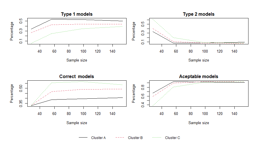
The results of Table 2 and Figure 1 clearly suggest that the percentage of acceptable models is associated with the sample size; the larger, the better the percentage of acceptable models. From sample size equal to 56, the percentages of acceptable models reach high levels, with small differences between the criteria, indicating that the procedure provides great results even for intermediate samples, regardless of the criteria adopted. These results suggest that, for acceptable models, the adopted criterion is not an important factor when we have large samples, since the procedure is robust to find acceptable models with high probability.

However, the same does not happen when we consider only the correct models. We noticed that, for sample sizes above 56, we have better results when we use the criteria associated with cluster C. The criteria included in this cluster have something in common, i.e., all of them use $\tilde{R}_{m}^{2}(\sqrt{n})$ to testing parameters associated with the mean model and does not use the $AIC_{c}$ to testing parameters associated with the dispersion model. This may be an indication that, for large samples and considering only correct models as a target, the use of $\tilde{R}_{m}^{2}(\sqrt{n})$ for mean models avoiding the $AIC_{c}$ for dispersion models should be encouraged.

For sample size equal to 28, we have a different scenario. We noticed that there is no cluster capable of increasing the proportion of correct models, but there is a cluster capable of increasing the proportion of Type 1 models and consequently increasing the proportion of acceptable models. This cluster is A; which also decreases the proportion of Type 2 models. The criteria included in cluster A always use $AIC_{c}$ to testing parameters associated with the dispersion model and does not use the $EAIC$ to testing parameters associated with the mean model. On this way, for small samples this may indicate that the use of $AIC_{c}$ for dispersion models avoiding the $EAIC$ for mean models would be the best option.

The bread-making problem, originally presented by Faergestad and Naes 1997, according to Naes et al. 1998, consisted of an experiment with three ingredients of mixture and two noise variables, and had as objective to investigate and to value the final quality of flour, composed by different mixtures of wheat flour, for production of bread. Also, according to Naes et al. 1998, Faergestad and Naes 1997 considered three types of wheat flour: two Norwegian, Tjalve $(x_{1})$ and Folke $(x_{2})$ and one American, Hard Red Spring $(x_{3})$, that were considered as control variables, and two types of process variables: mixing time $(z_{1})$ and the proofing (resting) time of the dough $(z_{2})$, considered as noise variables. The response variable was considered as the loaf volume after baking with target value of 530 ml. The flour blends were considered to be mixing ingredients with $x_{1}+x_{2}+x_{3}=1$ and with constraints $0.25\leq x_{1}\leq 1.0$; $0\leq x_{2}\leq 0.75$ and $0\leq x_{3}\leq 0.75$, where $x_{1}$, $x_{2}$ and $x_{3}$ are the proportions of Tjalve, Folke and Hard Red Spring flour, respectively. For the noise variables, it was considered three situations for the mixing time: 5, 15 and 25 minutes and also three situations for proofing time: 35, 47.5, and 60 minutes. The noise variables were coded as $-1$, 0, 1 according to their minimum, mean and maximum values.

A full $3^{2}$ factorial design was used for the noise variables and the 10 runs corresponding to a simplex-lattice design were replicated at each of the nine combinations of the mixing and proofing times, so the complete design involved 90 experimental runs as shown in Figure 2.

The volumes recorded for the 10 flour types and the 9 combinations of the noise variables are reproduced in Table 3. Additional details of the way in which the experiment was conducted are given by Naes et al. 1998, and further description of the practical aspects of the study is provided by Faergestad and Naes 1997 according to Naes et al. 1998.

Naes et al. 1998, considering Normal distribution and constant variance, carried out a study of the use of robust design methodology to the bread-making problem to investigate the underlying relationships between the response variable loaf volume and the mixture and noise variables, comparing three techniques for analysing the loaf volume, i.e., the mean square error, the analysis of variance and the regression approach, where all factors, the three mixtures components and the two noise variables, were modeled simultaneously. In the analysis considered by Naes et al. 1998 the dispersion was considered constant. However, when we use our variable selection procedure for this data set, we find that the dispersion is not constant. Thus, in this section, we reexamine the bread-making problem considering the possibility of obtaining, in addition to the mean model, a model for variance. For this, we will use the joint modeling of mean and dispersion, presented in Section 3.

For the application of the variable selection process, we considered $V(\mu)=1$ and identity link function for the mean model. For the dispersion model we considered the Gamma distribution with a logarithmic link function. The terms of the set $\cal{V}$, used in both the mean and the dispersion models, consisted of the terms of the cubic model in the mixture components crossed with the quadratic model in the noise variables.

In our application, the criterion considered for the mean model was the $\tilde{R}_{m}^{2}$ with $\lambda_{n}=\sqrt{n}$ and for the dispersion model the criterion was the $\tilde{R}_{d}^{2}$ with $\lambda_{n}=1$. These criteria were chosen due to the fact that we have a large sample, which indicates that the criteria in cluster C would be better. Among the criteria of cluster C, we chose those that have the highest percentage of correct models for large samples, according to Table 2.

Table 4 presents the results of all steps of the variable selection process (Algorithms 2 and 3) taken to obtain the final joint model for the mean and dispersion. The initial test, presented at the beginning of each iteration, for both the mean model and the dispersion model, concerns the hypothesis test to verify whether the model should have a constant term or not; thus, the null hypothesis states that the parameters of the main effects terms are equal to a constant value. In each iteration of Algorithm 2, Algorithm 3 was used to find the terms of the mean and dispersion models.

References

- Antoniadis et al. (2016) Antoniadis, A., Gijbels, I., Lacroix, S.L. and Poggi, J.M. (2016). Joint estimation and variable selection for mean and dispersion in proper dispersion models. Electronic Journal of Statistics, v. 10, pp. 1630-1676.
- Casella and Berger (2002) Casella, G., Berger, R. L. (2002). Statistical Inference, 2nd ed. Duxbury - Thomson Learning - New York.
- Cornell (2000) Cornell, J. A. (2000). Fitting a slack-variable model to mixture data: some questions raised. Journal of Quality Technology, v. 32, pp. 133-147.
- Cornell (2002) Cornell, J. A. (2002). Experiments with Mixtures: Designs, Models, and the Analysis of Mixture Data., 3rd ed. Wiley, New York.
- Cornell (2011) Cornell, J. A. (2011). A Primer on Experiments with Mixtures, ed. Wiley, New Jersey.
- Cornell and Gorman (2003) Cornell, J. A., Gorman J. W. (2003). Two new mixture models: living with collinearity but removing its influence. Journal of Quality Technology, v. 35, pp. 78-88.
- Dunn and Smyth (2018) Dunn, P. K., Smyth, G. K. (2018). Generalized Linear Models With Examples in R, Springer, New York.
- Faergestad and Naes (1997) Faergestad, E. M., Naes, T. (1997). Evaluation of baking quality of wheat flours: I: small scale straight dough baking test of heart bread with variable mixing time and proofing time. In: Report MATFORSK, As, Norway.
- Goldfarb et al. (2003) Goldfarb, H. B., Borror, C. M., Montgomery, D. C. (2003). Mixture-process variable experiments with noise variables. Journal of Quality Technology, v. 35, n. 4, pp. 393-405.
- Granato et al. (2020) Granato, D., Calado, V., Pinto, E. R. (2020). Optimization of food processes using mixture experiments - some applications. In Mathematical and Statistical Applications in Food Engineering, eds. S. Sevda and A. Singh, CRC Press, pp. 21-35.
- Gujarati and Porter (2009) Gujarati, D. N., Porter, D. C. (2009). Basic Econometrics, 5th. ed., McGraw-Hill/Irwin, New York.
- Johnson and Wichern (2019) Johnson, R. A., Wichern, D. W. (2007). Applied multivariate statistical analysis. Prentice Hall, New York.
- Jorgensen (2013) Jorgensen, B. (2013). Generalized linear models. In A. H. El-Shaarawi, & W. W. Piegorsch (Eds.), Encyclopedia of Environmetrics, Chichester: Wiley, ed., pp. 1152-1159.
- Khuri (2005) Khuri, A. I. (2005). Slack variable models versus Scheffé’s mixture models. Journal of Applied Statistics, v. 32, pp. 887-908.
- Lee and Koval (1997) Lee, K. I., Koval, J. J. (1997). Determination of the best significance level in forward stepwise logistic regression. Communications in Statistics - Simulation and Computation, v. 26, pp. 559-575.
- Lee and Nelder (1998) Lee, Y., Nelder, J. A. (1998). Generalized linear models for analysis of quality improvement experiments. The Canadian Journal of Statistics, v. 26, n. 1, pp. 95-105.
- Lee and Nelder (2003) Lee, Y., Nelder, J. A. (2003). Robust design via generalized linear models. Journal of Quality Technology, v. 35, n. 1, pp. 2-12.
- Marquardt and Snee (1974) Marquardt, D. W. and Snee, R. D. (1974). Test statistics for mixture models. Technometrics, v. 16, pp. 533-537.
- McCullagh (1983) McCullagh, P. (1983). Quasi-likelihood functions. The Annals of Statistics, v. 11, n. 1, pp. 59-67.
- McCullagh and Nelder (1989) McCullagh, P., Nelder, J. A. (1989). Generalized Linear Models, 2nd ed., Chapman and Hall, London.
- Montgomery (2017) Montgomery, D. C. (2017). Design and analysis of experiments, 9th. ed., Wiley, New York.
- Naes et al. (1998) Naes, T., Faergestad, E. M., Cornell, J. A. (1998). A comparison of methods for analyzing data from a three component mixture experiment in the presence of variation created by two process variables, Chemometrics and Inteligence Laboratory Systems, v. 41, pp. 221-235.
- Nelder and Lee (1991) Nelder, J. A., Lee, Y. (1991). Generalized linear models for the analysis of Taguchi-type experiments. Applied Stochastic Models and Data Analysis, v. 7, pp. 107-120.
- Nelder and Pregibon (1987) Nelder, J. A., Pregibon, D. (1987). An extended quasi-likelihood function. Biometrika, v. 74, pp. 221-232.
- Nelder and Wedderburn (1972) Nelder, J.A. and Wedderburn, R.W.M. (1972). Generalized linear models. Journal of the Royal Statistical Society, Series A, v. 135, 370-384.
- Pereira and Pinto (2021) Pereira, L. A., Pinto, E. R. (2021). stepjglm: Variable selection for joint modeling of mean and dispersion. R package version 0.0.1. https://cran.r-project.org/package=stepjglm.
- Piepel (1983) Piepel, G. F. (1983). Defining consistent constraint regions in mixture experiments. Technometrics, v. 25, n. 1, pp. 97-101.
- Piepel (2004) Piepel, G. F. (2004). 50 Years of mixture experiment research: 1955-2004, in Response Surface Methodology and Related Topics, ed. A.I. Khuri, World Scientific Publishing, Singapore, pp. 283-327.
- Piepel and Cornell (2001) Piepel, G. F., Cornell, J. A. (2001). A catalogue of mixture experiment examples. BN-SA-3298, Battelle, Pacific Northwest Laboratories. Richland, WA.
- Pinto and Pereira (2021) Pinto, E. R., Pereira, L. A. (2021). On variable selection in joint modeling of mean and dispersion. Brazilian Journal of Probability and Statistics, v. 35, n. 4, pp. 875-894.
- R Core Development Team (2019) R Development Core Team (2019). R: A language and environment for statistical computing. R Foundation for Statistical Computing, Vienna, Austria, URL http://www.R-project.org.
- Scheffé (1958) Scheffé, H. (1958). Experiments with mixture. Journal of the Royal Statistical Society B, v. 20, pp. 344-366.
- Smith (2005) Smith, W. F. (2005). Experimental design for formulation. New York: Society for Industrial and Applied Mathematics - SIAM, New York.
- Steiner and Hamada (1997) Steiner, H. S., Hamada, M. (1997). Making mixtures robust to noise and mixing measurement errors. Journal of Quality Technology, v. 29, n. 4, pp. 441-450.
- Taguchi (1986) Taguchi, G. (1986). Introduction to Quality Engineering, Unipub/Kraus International Publications, White Plains, New York.
- Wang and Zhang (2009) Wang, D., Zhang, Z. (2009). Variable selection in joint generalized linear models. Chinese Journal of Applied Probability and Statistics, v. 25, pp. 245-256.