A field equation for induction-transduction of activation-deactivation probability on measurable space

Let $\phi_{x}(y)\equiv\phi(x,y)$ and $I$ be the identity function. The point activation degree function (random density field) is given by the image

Put $f_{x}(\cdot)\equiv f(x,\cdot)$. The degree function has probability generating function (pgf), mean, variance, covariance, and correlation

For $a>0$, both of these choices for $f$ result in decreasing degree functions $d$. In the first case, the normalized degree function is one at zero, $\nu(f_{0})=1$, so these points have maximum mean activation degree. For the second, the normalized degree function is less than one at zero, $\nu(f_{0})=\varphi_{U}(a)<1$, so these points have mean degree less than the maximum.

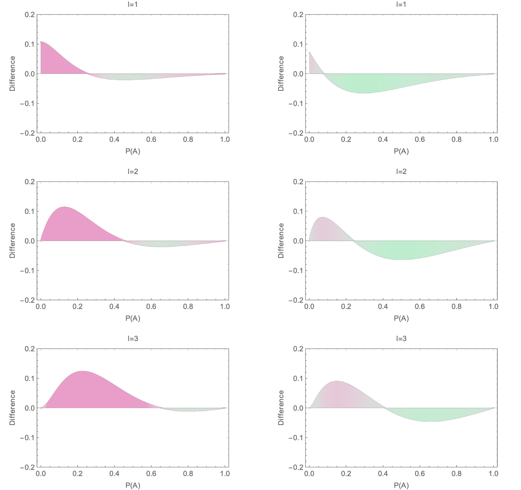
An interesting special case is constant density kernel $f(x,y)=p$ and fixed number $c$ of points, $\kappa=\text{Dirac}(c)$. Then ${\symAMSb C}orr(d(x),d(y))={\symAMSb I}(x=y)$. Hence for the constant density kernel $f=p$ and a fixed number of points $c$, the activation degrees (densities) are decorrelated $\text{Binomial}(c,p)$ random variables. For $\kappa=\text{Poisson}(c)$, then ${\symAMSb C}orr(d(x),d(y))={\symAMSb I}(x=y)+p{\symAMSb I}(x\neq y)$. Hence the Poisson random measure ($c=\delta^{2}$) correlates the density field. More generally, the Poisson-type (PT) random measures correlate the degree function, with binomial ($\delta^{2}<c$) and negative binomial ($\delta^{2}>c$) respectively having reduced and increased correlation relative to Poisson, and binomial recovering Dirac as $\delta^{2}\rightarrow 0$. We illustrate the degree function correlations of the constant density kernel for the PT random measures below in Figure 1. The constant density kernel demonstrates that the correlation structure of the point activation density is determined by both the density kernel $f$ and the point counting law $\kappa$.

We say a point $X$ is in activation when $d(X)\geq k$ for some $k\geq 1$, and its vertex is said to be $k$-active. The number of $k$-active vertices

corresponds to the number of points in activation and has mean

where

Consider a point system of $K\sim\kappa=\text{Poisson}(c)$ points with $c=50$. Consider the Bernoulli random graph $G(\phi)$ with density kernel $f$. We choose $f$ as $f_{1}(x,y)=a_{1}$ for $a_{1}\in(0,1]$, $f_{2}(x,y)=\exp_{-}a_{2}xy$, and $f_{3}(x,y)=\exp_{-}a_{3}(x+y)$, where $a_{2}$ and $a_{3}$ are chosen such that $a_{1}=(\nu\times\nu)f_{2}=(\nu\times\nu)f_{3}$, i.e. $f_{1},f_{2},f_{3}$ have the same normalized edge density. We take $a_{1}=1/10$, giving $a_{2}\simeq 43.4997$ and $a_{3}\simeq 3.0057$. We simulate $V_{k}(G)$ 10,000 times for $k=8$ for each kernel, plot the empirical distributions below in Figure 2, and report their sample statistics in Table 2. Despite the fixed mean total number of activation interactions, the resultant random variables $V_{k}(G)$ have markedly different distributions. Firstly, the constant kernel has the smallest mean and by far the largest probability of zero activations. The kernels $f_{2}$ and $f_{3}$ give small probability to zero activations, with the mean and variance of $f_{2}$ dominated by those of $f_{3}$, and $f_{2}$ has the smallest variance of the three considered kernels. We plot degree covariance and correlation for $f_{2}$ and $f_{3}$ in Figure 3, conveying distinct structures. We show random graphs $G_{1},G_{2},G_{3}$ corresponding to the three kernels in Figure 4. These illustrate the qualitative differences between the homogeneous structure of $f_{1}$ and the non-homogenous structures of $f_{2}$ and $f_{3}$. For instance, $G_{2}$ contains one highly connected point and a number of disconnected points, whereas $G_{1}$ is a connected homogeneous Poisson graph.

Consider $N=(\kappa,\nu)$ on $(E,\mathscr{E})=([0,1],\mathscr{B}_{[0,1]})$ with $\nu=\Leb$ formed by independency $\mathbf{X}$ and its product random measure $M=N\times N$ with symmetric Bernoulli transformation $\phi$ and degree function $d(x)=N\phi(x,\cdot)$. Suppose we have mark-space time-set $[0,T]$. The idea is that each point is identified to location in $E=[0,1]$ with distribution $\nu=\Leb$ and a time-of-arrival (TOA) of the location in $[0,T]$ with distribution $\pi=\text{Uniform}[0,T]$. This is a simple marked random measure design where TOA and locations are independent. Let independency $(\mathbf{X},\mathbf{T})$ form the random measure $N^{*}=(\kappa,\nu\times\pi)$ on $(E\times[0,T],\mathscr{E}\otimes\mathscr{B}_{[0,T]})$. Define the time-dependent point activation degree function

Then we can define the point activation process as

The mean carries over in a manner similar to those of the system activation distribution based on marked random measures. In this setting, $(d_{t}(x,s))_{t\in[0,T]}$ is a non-decreasing, pure-jump, counting process for every $(x,s)\in E\times[0,T]$, with initial condition $d_{0}(x,s)=0$ and terminal condition $d_{T}(x,s)=d(x)$. Similarly, $(V_{k}^{t}(G))_{t\in[0,T]}$ is a non-decreasing, pure-jump, counting process. They are both non-decreasing because they both may be the zero process. An immediate generalization is taking the TOA distribution $\pi$ to be non-uniform. Note that these processes are neither Lévy nor Markov, even for Poisson $N^{*}$. A further generalization is letting the activation value and TOA be dependent.

We have defined points in activation in terms of their degree functions, formed from edge counts. Instead, we can define points in activation in terms of higher-order edge relations, such as relative to the number of triangles the points participate in or other motifs.

A number of generalizations are possible. The transformation need not be symmetric, yielding directed graphs. Then the points have in- and out-degrees. Also the transformation can be a choice different from Bernoulli, such as Poisson (giving activation multigraphs). Others are randomizing the threshold $k$ in the threshold function ${\symAMSb I}_{\geq k}$ or considering a general non-negative (possibly random) function. The mark space law can be described through a transition kernel, encoding conditional dependence on location. The location space can be multi-dimensional, incorporating point attributes, etc.

Let $g_{xy}(x^{\prime},y^{\prime})\equiv g((x,y),(x^{\prime},y^{\prime}))$. Define the activation degree function as

The degree has mean

and pgf

We say that the deactivation point $(X_{i},Y_{i}=D)$ is in activation if $d_{B}(X_{i},Y_{i})\geq l$ for $l\geq 1$. The number of activations is

with mean

where

and $d_{B}(x,D)$ has pgf

The spatial-temporal induction-transduction activation-deactivation (ITAD) field equation on $(F,\mathscr{F})=([0,1],\mathscr{B}_{[0,1]})^{{\symAMSb R}_{\geq 0}\times E}$ is given by the following spatio-temporal ordinary differential equation

The induction-transduction activation field equation is retrieved by taking $m=\infty$ such that

For the case of Poisson and unit thresholds $k=l=m=1$, the ITAD field equation is given by

The field equation can be solved in discrete-time as

For example the density function has distribution

where the contour integral is over the unit circle $C$. These calculations can be unstable or expensive. Towards efficiency, notice that the density pgfs $\psi_{x}$, $\psi_{xu}^{D}$, and $\psi_{xu}^{A}$ are each binomially thinned. If the counting law is closed under binomial thinning, then the density distributions are rescaled versions of themselves, i.e. they are self-similar, and there is no need for differentiation nor complex integration. Alas, it turns out on diffuse space that there are only three self-similar members of the canonical non-negative power series family of distributions to possess closure under binomial thinning, the Poisson-type (PT): Poisson, negative binomial, and binomial. The Dirac measure can be said to be a fourth, as the limit of the binomial distribution. This means that systems having fixed or PT cardinality possess self-similar configurations. Note that the PT random measures are also closed under thinning for atomic measures, but not uniquely so. For completeness the PT family of distributions are given by

and the rescalings to subspace $A\subseteq E$ with mass $a$ are given by

The Poisson-type distributions can be approximated by Gaussian when the degrees are large. Putting $a_{x}=\nu(f_{x})$, we have (with some abuse of notation)

The (marginal) temporal field equation is attained as the following ordinary differential equation

The equation can be solved in discrete-time as

Assuming $\nu$ is diffuse, the associated (first-order) wave equation on $(W,\mathscr{W})=({\symAMSb R},\mathscr{B}_{{\symAMSb R}})^{{\symAMSb R}_{\geq 0}\times E}$ is given by

where $C_{1}>0$ is an appropriately dimensionalized constant, e.g., transport velocity.

Consider $E=[0,1]$. The energy equation on $(G,\mathscr{G})=({\symAMSb R},\mathscr{B}_{{\symAMSb R}})^{{\symAMSb R}_{\geq 0}\times E}$ is given by

where $C_{2},C_{3}>0$ are appropriately dimensionalized constants, e.g, $C_{2}$ and $C_{3}$ are the mass density and tension of a unit length vibrating string.

The entropy field is

The maximum entropy activation frontier (or activation event horizon) is given by the level set

The field equation can be extended to include forcing and overloading through non-negative forcing parameters $(a,b)$ and overloading parameters $(\alpha,\beta)$, i.e.,

The forcing-overloading pairs for activation $(a,\alpha)$ and deactivation $(b,\beta)$ are chosen such that $\sup_{(x,u)\in E\times[0,1]}(\alpha q_{l}(x,u)+a)\leq 1$ and $\sup_{(x,u)\in E\times[0,1]}(\beta r_{m}(x,u)+b)\leq 1$ respectively hold.

For continuous marginal density functions (‘sources’), i.e. $\nu(f_{x})$ is continuous on diffuse $(E,\mathscr{E})$, the ITAD field equation can be provisioned as a continuous wave equation. The ITAD wave equation, with forcings $a$ and $b$, is given by

where $C_{1}\geq 0$ is activation transport velocity. If $C_{1}=0$, then the standard ITAD field equation is retrieved. The additional term processes the field fluctuations relative to finite activation transport velocity. Note that, for given activation-deactivation transduction thresholds $l$ and $m$, the forcings $a$ and $b$ must be chosen such that $\sup_{(x,u)\in E\times[0,1]}(q_{l}(x,u)+a)\leq 1$ and $\sup_{(x,u)\in E\times[0,1]}(r_{m}(x,u)+b)\leq 1$. Solution stability exhibits a bifurcation in $C_{1}$, where increasing $C_{1}$ beyond a certain level causes the ITAD wave equation to blow-up in finite-time. The ITAD wave equation can also be solved in discrete time and/or space, employing suitable finite differences.

We think of $f$ in $(\mathscr{E}\otimes\mathscr{E})_{[0,1]}$ as a density function or kernel. We discuss four archetypical ITAD mechanisms for $E=[0,1]$ and $\nu=\Leb$: central, subcentral, decentral, and local. We denote $\varphi_{U}(\alpha)=(1-e^{-\alpha})/\alpha$ the Laplace transform of the uniform distribution on $[0,1]$.

References

- Baron and Wesolowski, (2021) Baron, K. and Wesolowski, J. (2021). From Invariance Under Binomial Thinning to Unification of the Cauchy and the Golab–Schinzel-Type Equations. Results in Mathematics, 76(4):168.
- Bastian and Rabitz, (2022) Bastian, C. and Rabitz, H. (2022). Random graphs by product random measures.
- Bastian and Rempala, (2020) Bastian, C. D. and Rempala, G. A. (2020). Throwing stones and collecting bones: Looking for Poisson-like random measures. Mathematical Methods in the Applied Sciences, 43(7):4658–4668.
- Cinlar, (2011) Cinlar, E. (2011). Probability and Stochastics. Springer-Verlag New York.
- Di Lauro et al., (2022) Di Lauro, F., KhudaBukhsh, W. R., Kiss, I. Z., Kenah, E., Jensen, M., and Rempała, G. A. (2022). Dynamic survival analysis for non-Markovian epidemic models. Journal of The Royal Society Interface, 19(191):20220124.
- Gaveau et al., (1984) Gaveau, B., Jacobson, T., Kac, M., and Schulman, L. S. (1984). Relativistic Extension of the Analogy between Quantum Mechanics and Brownian Motion. Phys. Rev. Lett., 53:419–422.
- Ornstein, (1970) Ornstein, D. (1970). Bernoulli shifts with the same entropy are isomorphic. Advances in Mathematics, 4(3):337–352.
Appendix A Induction-transduction