Entropy and entanglement in a bipartite
quasi-Hermitian
system and its Hermitian counterparts
Abstract
We consider a quantum oscillator coupled to a bath of other oscillators. The total system evolves with a quasi-Hermitian Hamiltonian. Associated to it is a family of Hermitian systems, parameterized by a unitary map . Our main goal is to find the influence of on the entropy and the entanglement in the Hermitian systems. We calculate explicitly the reduced density matrix of the single oscillator for all Hermitian systems and show that, regardless of , their von Neumann entropy oscillates with a common period which is twice that of the non-Hermitian system. We show that generically, the oscillator and the bath are entangled for almost all times. While the amount of entanglement depends on the choice of , it is independent of when averaged over a period. These results describe some universality in the physical properties of all Hermitian systems associated to a given non-Hermitian one.
1 Motivation & outline of main results
In recent years there has been much interest in extensions of quantum mechanics that allow for non-Hermitian Hamiltonians. In -symmetric quantum theory, for instance, non-Hermitian Hamiltonians with purely real spectrum are often encountered. In many cases those Hamiltonians are quasi-Hermitian [1, 2, 3, 6, 20, 21, 22, 23, 26, 29]. For these one can produce associated Hermitian Hamiltonians which can then be studied using ‘standard’ methods of quantum theory.
The assignment of a Hermitian to a non-Hermitian system is called the Dyson map [12, 8, 9]. The Dyson map is determined up to a unitary. To a given non-Hermitian Hamiltonian are assigned Hermitian Hamiltonians which are all unitarily equivalent. In this sense, physical properties of the original are uniquely encoded by any associated . However, if the system has a subsystem structure, then the unitaries generally reshuffle local degrees of freedom and the choice of the unitary plays a crucial physical role. This is in particular the case for open systems, where system and bath degrees of freedom are reshuffled. One should then ask what relevant information about the original non-Hermitian system is encoded in ‘the’ associated Hermitian one. In fact, if one allows the Dyson map to be time-dependent, as is often the approach taken in the literature [11, 12, 14], then the above mentioned non-uniqueness is compounded by additional freedom. It turns out that given any quasi-Hermitian system , one can chose a suitable time-dependent Dyson map so that the associated Hermitian system has the trivial Hamiltonian . We explain this in Appendix A.3.
The ambiguity in the associated Hermitian systems is the subject of the present paper. In the recent literature on -symmetric quantum theory it is suggested that instead of studying the entropy of an open quasi-Hermitian systems, one may study the entropy of the corresponding associated Hermitian system [13, 17, 18, 5]. Concretely, in [13], the authors examine the entropy of an oscillator coupled to an ‘environment’ of other oscillators via a -symmetric Hamiltonian. As a proxy for the von Neumann entropy of the single oscillator in the non-Hermitian system, they study the corresponding quantity for one particular choice of an associated Hermitian system, constructed by a time-dependent Dyson map. The authors find a different qualitative behaviour of the entropy of the Hermitian system according to the -symmetry phases of the non-Hermitian system. This interesting result is found for one particular choice of the associated Hermitian system – the choice may be regarded as a good one as it discerns the different symmetry phases by the qualitative form of the dynamics of the entropy. For a different choice however, the entropy dynamics would look entirely different (and in particular, it would be time-independent upon chosing , as explained above).
In the current work we investigate all associated systems in the regime of unbroken -symmetry – in which the non-Hermitian Hamiltonian is actually quasi-Hermitian. We vary over all time-independent Dyson maps (excluding time dependent ones for the reason mentioned above).
A Hamiltonian is said to be quasi-Hermitian if
for some bounded, positive operator , called a metric operator. One obtains a Hermitian Hamiltonian by
where is any operator with
The assignment is called the Dyson map [8, 9], even though to a single one can associate different for the following two reasons.
- –
There are different metric operators for the same quasi-Hermitian .
- –
Once a metric is fixed, the general solution of the equation is , where is the unique positive operator that squares to and is an arbitrary unitary .
The metric is uniquely determined if one fixes a sufficiently rich (irreducible) set of quasi-Hermitian operators (including ) to be observables; see [29] and Section 2. Once this choice is made, all associated Hermitian systems are parameterized by the unitary . Different choices of give different Hermitian , which are unitarily equivalent. However, generally reshuffles the degrees of freedom and modifies local physical properties, such as entanglement between subsystems.
In this work, we consider a concrete quasi-Hermitian system with Hamiltonian , describing the interaction of a single oscillator with a bath of other oscillators. This is an open quantum system of the ‘system–bath’ () type, described by a bipartite Hilbert space . We take the metric to be general but fixed, and then analyze all the associated Hermitian systems resulting from varying over all choices of . The dynamics of the non-Hermitian system and associated Hermitian systems is given by the time-dependent wave functions
respectively. The vector is normalized with respect to the metric induced by the inner product , while is normalized relative to the ‘original’ inner product . The reduced density matrices for the non-Hermitian and the Hermitian systems are obtained by taking the partial trace over the bath degrees of freedom (see Section 2.2),
Our main findings are summed up as follows:
- 1.
- 2.
Metric . The operator is a density matrix exactly when is of product form – otherwise has complex eigenvalues. See Section 3.1. We thus take of product form in the further analysis.
- 3.
Subsystem entropy. The reduced states and are periodic11 1 The whole complex consists of oscillators, so the energy spectrum of all the Hamiltonians involved consists of discrete eigenvalues only, without continuous spectrum. This explains the periodicity. in time, both having the same period regardless of the choice of . The von Neumann entropy of and is periodic in time as well, but for generic initial conditions22 2 Only for specially tuned initial states and ’s is the situation non-generic, see Section 3.3. and generic , the period of the entropy of the Hermitian system is double that of the non-Hermitian system. See section 4.
- 4.
entanglement. The non-Hermitian and the Hermitian states , are entangled for all times except at periodically reoccurring single instants.33 3 For a class of exceptional initial conditions the states are entangled for all times, see Section 5. Given any entangled state , one can find such that the associated is disentangled, and for any disentangled there are such that is entangled. However, in an averaged sense, the choice of does not influence the entanglement at all. Namely, the concurrence of the time-averaged density matrix, , where is the period of , is independent of . Its value is determined entirely by the initial condition and the choice of the metric. We identify the initial states for which is separable and for which it is maximally entangled. See Section 5.
2 Quasi-Hermitian systems
Let be a finite-dimensional Hilbert space with inner product . An operator is said to be positive, denoted as , if for all nonzero . This is equivalent with saying that and all eigenvalues of are strictly positive. Here is the adjoint of the operator , defined by for all . An operator on is called (-)quasi-Hermitian if there exists a positive operator such that
| (1) |
Quasi-hermiticity is a special case of pseudo-hermiticity, where (1) holds with an invertible (but not necessarily positive) Hermitian operator . Pseudo- and quasi-hermitian Hamiltonians arise in -symmetric quantum theory, see for instance [31] and references therein.
2.1 Hermitian counterparts
Let be a non-Hermitian operator on , a candidate for the Hamiltonian of a physical system. In order to obtain a Hermitian quantum theory, one could either:
- (1)
Modify the inner product of to for some (called a metric operator), such that becomes Hermitian in the Hilbert space with this new inner product; or
- (2)
Take a similarity transformation (invertible map) such that the transformed is Hermitian in the original Hilbert space .
If is quasi-Hermitian, then both options (1) and (2) are possible, but neither the metric nor the similarity transform in options (1) and (2) are unique. To explore this non-uniqueness, we first notice that any quasi-Hermitian is diagonalizable [7, 10, 21]. More precisely,
| (2) |
where the are the eigenvalues and the form a complete bi-orthonormal family, meaning that and . Let us consider the case where all eigenvalues are distinct for simplicity (a discussion including degenerate eigenvalues can be done similarly, but this is not our focus here). Then the decomposition (2) is unique, it is the spectral representation of the operator , and the are the uniquely defined (generally not orthogonal) spectral projections. The vectors and , however, are determined only up to a joint scaling and , with arbitrary.
First let us explore the option (1). A metric is called a metric for if is -quasi-Hermitian. Let be a linear operator on , with adjoint as defined above. If is viewed as an operator on , then , so the adjoint of in is . It follows that a given is a metric for if and only if , that is, if and only if is Hermitian acting on . It is well known (see e.g. [26, 10]) that
| (3) |
where the are the vectors appearing in (3). The multitude of metrics obtained by varying the in (2) naturally appears due to the fact that is only determined up to an arbitrary nonzero scaling factor (as explained after (2)), which results in the scaling . Given this non-uniqueness of the metric, which one should be chosen to define the physical Hilbert space ?
One answer is that the metric is fixed provided that instead of just , one chooses a whole irreducible family of operators to be Hermitian observables. Namely, it is shown in [29] (see also [25] for the two-dimensional case) that if there is a family of operators on , and positive operators , such that and for all , then
This means that for an irreducible family of quasi-Hermitian operators, there is exactly one metric (up to a scalar multiple) that makes those operators Hermitian. The chosen family44 4 Examples of irreducible families are the Pauli matrices for a spin, with the Euclidean inner product on , or the position and momentum for a quantum particle (rather, the bounded Weyl operators generated by them) with the inner product . can then be viewed as the physical observables of the theory and the space of pure states is with inner product .
On the other hand, if interested only in the single observable (the Hamiltonian), one should keep the in (3) general.
Next, let us investigate option (2) for of the form (2). Let be a metric for , so it is of the form (3). We find all invertible such that the transformed is Hermitian,
| (4) |
One readily sees that (4) is equivalent to , where . That commutes with , as in (2), is equivalent to being diagonal in the same bi-orthonormal system as , that is, for some . Now
| (5) |
and as and , we have as well. It follows from (3) and (5) that is also a metric for . In fact, (3) and (5) show that given a fixed metric for and varying over all operators that commute with , we obtain all of the metrics for . We conclude that given , the we are looking for are the solutions of , where is an operator that commutes with (equivalently, is diagonal in the same bi-orthonormal system as ). The general solution is
| (6) |
where is any unitary and where for a positive operator , is the unique positive operator whose square equals .
Once and are chosen, the associated Hermitian in (4) becomes
| (7) |
We stress with this notation that depends on the choice of and . The obtained from two different choices of unitaries, say and , are unitarily equivalent, with and . In this sense, the choice of is globally immaterial. However, if the Hilbert space has a local structure, say is of bipartite nature , then the global unitary may well change the local properties of the two local subsystems, in which case the choice of will play a physically relevant role. We also point out that the spectrum of does not depend on either or (or , for that matter).
In this work we take the following approach: We start with a given quasi-Hermitian Hamiltonian and an arbitrary metric for and we view as the physical Hilbert space. We analyze the class of all associated Hermitian systems , where and vary over all unitaries and all positive operators commuting with , respectively. As explained above, considering all metrics is the same as considering all metrics , so varying over is redundant if is kept arbitrary. We may then set and only consider
| (8) |
for all and .
2.2 States, reduced states, von Neumann entropy
Consider now a fixed metric , so that the physical Hilbert space is and is Hermitian on , . Then is the unitary Schrödinger dynamics on . The average of an observable on in the state is given by
| (9) |
where
| (10) |
is a density matrix on (a positive, trace-one operator). This is called the ‘generalized density matrix’ in [28]. It is important to point out that the trace in (9) is a purely algebraic quantity: it is the sum of the eigenvalues of the operator, and therefore does not depend on the choice of metric.
To arrive at a Hermitian Hamiltonian, it is necessary to make a choice for the unitary in (8). The associated Hermitian Hamiltonian is then given by (8). Let
| (11) |
be the evolution of the initial states , with respect to and , respectively. The states are related by
| (12) |
and the density matrices associated to these vector states for the non-Hermitian (see (10)) and the Hermitian systems are
| (13) |
respectively. (We adopt the notation and for the density matrices on the Hermitian and non-Hermitian sides of the problem from [13].) It is clear from (12) that
| (14) |
It follows that and have the same eigenvalues, and hence the same von Neumann entropy, , where
| (15) |
and are the eigenvalues of .
Consider now a bipartite system with (‘system’ and ‘bath’). We consider the reduced states (denoted by an overbar) defined by tracing out the degrees of freedom of the subsystem ,
| (16) |
In some recent works [13, 17, 18, 5], the dynamics of a bipartite system generated by a non-Hermitian Hamiltonian is studied, with particular focus on the von Neumann entropy of the reduced density matrix . The strategy proposed in those works is to examine the entropy of as a proxy for that of . In this respect, however, one should observe the following facts:
- 1.
The operator always satisfies , but for some choices of the eigenvalues of can be complex, in which case it is not a valid density matrix.
- 2.
Even if the metric is chosen such that is a density matrix, for generic choices of the von Neumann entropies and are not the same. The latter in fact depends on the choice of .
To understand the normalization of the trace mentioned in fact 1. above, we observe (using as the system observable) that
If , then and so the spectra and thus the von Neumann entropies of and coincide. However, if is entangling (not of product form ), then the eigenvalues of the two reduced density matrices are not the same in general, and neither are their entropies.
These difficulties are resolved in the next section, where we study the concrete model used in [13]. In particular, we determine for which choices of the reduced operator is indeed a density matrix, and then we find the von Neumann entropy of for all possible choices of the unitary .
3 Model
An oscillator with creation and annihilation operators , is coupled to a ‘bath’ of independent oscillators with creation and annihilation operators , , . The total Hilbert space of the oscillators is
| (17) |
where is the space of a single oscillator and is that of the other . As in the previous section, we denote the inner product by and let denote the adjoint in this inner product. The commutation relations are , and all operators belonging to different oscillators commute. This open quantum system, non-Hermitian model was used in [13].
3.1 The quasi-Hermitian system
The coupled total system–bath Hamiltonian is
| (18) |
where and are parameters and
| (19) |
Due to the different prefactors of in the interaction term of (18), is -Hermitian if and only if .
The ‘uncoupled’ () Hamiltonian is simply , a multiple of the total number operator . As commutes with , each eigenspace of , with a fixed number of excitations (in the system plus the bath) is left invariant. Denote by the ‘vacuum’ zero excitation state, where all oscillators are in the ground state. The single excitation space is defined as
| (20) |
where and for . When is applied to a vector in the result is again a vector in . Moreover, due to the collective, symmetric nature of the system-bath interaction in (18), leaves the even smaller space
| (21) |
invariant, where
| (22) |
Those two vectors describe states in which a single excitation is either in (the state ) or in , collectively spread over the bath oscillators (the state ). Therefore, we may view as an operator on . When we do this we denote it by , which has the form
| (23) |
The eigenvalues of are
| (24) |
which are real for and (purely imaginary) complex conjugates for . See [13] for a discussion of the symmetry of . The operator is diagonalizable except at the transition points defined by , where reduces to a Jordan block. Note that increasing the number of oscillators in the bath simply amounts to speeding up the dynamics (the frequency ) by a factor .
We consider the ‘-symmetry unbroken regime’ , so that . For definiteness we take (the case can be dealt with in the same fashion), so
| (25) |
which is equivalent to and . Then we have and
| (26) |
where the equalities in (26) define the quantities , . The two linearly independent (not normalized) eigenvectors of and its adjoint are
respectively. They satisfy and . Note that denote the eigenvectors of , not to be confused with the complex conjugates of the eigenvectors of . We normalize the vectors as
| (27) |
Then is a bi-orthonormal basis, satisfying and , and the operator can be written as
| (28) |
Using this, one easily finds
| (29) | |||||
We consider initial states which are vectors in , as defined in (21), so the dynamics generated by is entirely given by the operator from (23). We still consider the regime (25), so that the spectrum of consists of two distinct real eigenvalues. Comparing (2), (3) and (28), we see that is quasi-Hermitian and the set of all associated metrics is
| (30) |
Written as a matrix in the basis , we obtain from (27)
| (31) |
This is diagonal exactly when . As we will see in Section A.1, this is equivalent to being the restriction to of a product metric on . And as we discuss below after (39), this is also equivalent to the reduced system state in (38) being a positive operator.
3.2 Reduced non-Hermitian system dynamics
Fix an and take an initial state of the form
| (32) |
for some normalized to have , that is,
| (33) |
The dynamics is given by
| (34) |
where
| (35) | ||||
The normalization
| (36) |
holds for all , as acts unitarily on equipped with the inner product . The relation (36) is the same as (33) with and replaced by and .
We now introduce the reduction of the system to the single oscillator (, ). The average of a system observable (observable of the single oscillator) in the state given by (34) evolves according to
| (37) |
where the reduced system state is
| (38) |
For the partial trace we have the identities , and . Using (34) and of the form (30), we obtain after a calculation
| (39) | |||||
This matrix is diagonal in the basis and the two diagonal entries are its eigenvalues. One checks directly that (the sum of the diagonal elements equals ). However, the eigenvalues of are complex, in general, unless the metric is chosen to satisfy . Indeed, the imaginary part of the first eigenvalue is . If , the coefficients in the initial state (32), are real then this quantity becomes55 5 Use the equations (35) and write as a function of according to the normalization condition (33). . Unless or the initial condition satisfies , the eigenvalues of will not be real except at the discrete set of times when .
We require to be a density matrix (and in particular to have non-negative eigenvalues) for all times. To do so with a metric that does not depend on the initial conditions we therefore must choose . We thus take
for the remainder of the paper. In the basis the metric is diagonal,
| (40) |
see (31). As explained after (31) above, this is equivalent to being of product form. With this choice, given by (39) is -Hermitian. According to (39) and (35) we have
| (41) |
where
| (42) | |||||
In the last step, we used the normalization condition (33), resulting in , and the trigonometric identities , and . In view of (42) it is natural to introduce the parameter
| (43) |
Properties of :
- 1.
and depend on time unless and , in which case and .
- 2.
Otherwise and are periodic in time, with period , and the mean value of is
(44)
3.3 Reduced Hermitian system dynamics
Next, we turn our attention to the density matrix of the Hermitian system, which according to (14) is
| (45) |
We keep in the notation to highlight that the choice of depends on , see (8). Again choosing a metric of the form (30) with , we use (34) to obtain
| (46) |
where
| (47) |
We then obtain
| (48) |
written in matrix form in the ordered basis of . Next, we take a general (time-independent) unitary on , expressed in the same basis as
| (49) |
Using (45), (48), (49) and writing momentarily for , we get
| (50) |
We observe that is periodic in time, with period . This follows from (47) together with (35), since , and all have period .
Next we calculate the reduced density matrix of by taking the partial trace of over ,
| (51) |
where and are given in (47). We get the expression
| (52) |
where and are given in (35). Expanding the square and using as well as the normalization (33) (which is valid for replaced by at any time), we obtain
| (53) | |||||
where is the population of evaluated above in (42). Expanding the real part term in (53) using (35), we arrive at
| (54) | |||||
We take into account (42) to rewrite
| (55) | |||||
where we recall that is given in (43). Using the explicit form (55) of , we obtain the following information.
Properties of :
Generic initial states and unitaries. As , the average equals exactly when . This is a condition on the initial state (via ) and the unitary (via ). We call the initial state and the unitary generic, respectively, when
| (57) |
In other words, for generic initial states and unitaries, the average of the population of differs from the average of the population of . As we show in the next section, this deviation from the value causes the entropy of to oscillate with exactly half the frequency of the entropy of .
4 Entropy
Recall that the states and are given in (41) and (51), with associated populations , evaluated in (42) and (55). Their von Neumann entropy is given by
| (58) |
We show in Appendix A.2 that
If , then according to (44) and (56) the averages and around which the populations and oscillate are different for all generic initial conditions, i.e., all coefficients satisfying . This translates into a modification of the period of the entropy of as a function of time relative to that of , as we explain now.
4.1 Period doubling of von Neumann entropy in the non-Hermitian versus the Hermitian system
Consider the function
Suppose now that depends periodically on time and has average ,
| (59) |
with having period and zero average. This setup incorporates both cases and in one. As Figure 1 illustrates, if , which is the value where takes its maximum, then as moves over one period, the entropy moves over two periods.


On the other hand, if , then the period of the entropy is not doubled relative to that of , as Figures 2 and 3 show.


We draw the following conclusions:
-
The period of the von Neumann entropy of the non-Hermitian system is , regardless of the initial condition (except for the stationary state).
-
Regardless of the metric (parameter ), the period of the von Neumann entropy of the Hermitian system is:
-
, provided (generic case),
-
, provided (special case).
-
This means that for generic initial conditions (meaning ) and generic choices of the unitary (meaning ), the period of the von Neumann entropy of the Hermitian system is double that of the non-Hermitian system. That is, the entropy of the non-Hermitian system oscillates faster. This is so even though the populations in both cases have the same frequency . The change of the period is due to the shift of the average in the population induced by , as given in (56).
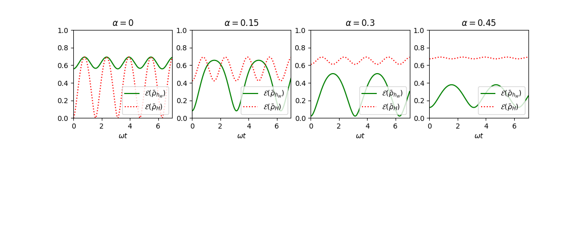
4.2 Numerical illustration of the period doubling
We plot the populations and entropies for parameters in the regime
| (60) | |||||
| (61) | |||||
| (62) |
According to (61) and the unitarity of , we have . Moreover, , where . The population of the Hermitian system reduced density matrix, given in (55), then becomes
| (63) |
with
| (64) | |||||
| (65) |
Here, and can be chosen freely. The population of the non-Hermitian system, in (42), is simply the expression (63) with .
Note that the change leaves invariant and flips the sign of . It then suffices to plot graphs for . For we get , which gives a stationary state (for all ). The same invariance of and sign flip of is induced by .
In Figure 4, we compare the von Neumann entropies of the two density matrices and , directly seeing the doubling of the period.
5 Entanglement of system and bath oscillators
The total Hilbert space in (17) is bipartite, one part being the singled-out oscillator (system), the other being the remaining oscillators (bath). We say that a nonzero vector is of product form, or disentangled, if for some and some . We call a nonzero entangled if it is not of product form. The notion of being entangled or not does not depend on the metric determining the inner product of . Nevertheless, the physical interpretation of entanglement in terms of independence of the subsystems and does depend on the metric. The physical manifestation of disentangled states is the independence of the two subsystems and . Namely, if the inner product of is given by a metric of the form (a particular example being ), then measurement outcomes of observables on either of the subsystems are independent random variables. This follows because expectation values of observables in a state split into products,
However, those random variables become dependent (correlated) if is not of product form, because then their average will not split into a product of a system term times a bath term.
In the model defined in Section 3, the metrics we consider are restrictions to the subspace of product metrics of (c.f. (31) and Section A.1). The physical meaning of entanglement in terms of subsystem independence does therefore not depend on the choice of within this class. In other words, measurement outcomes of system and bath observables in are independent or dependent, according to whether is disentangled or not, regardless of the choice of . It is then sensible to investigate the SB entanglement in pure states belonging to the subspace for all .
Any vector is of the form
| (66) |
In accordance with (22), we may write and . Explicitly, are the ground state and first excited state of the system oscillator, and are the ground state of all the bath oscillators and the distributed excitation state , respectively; see (22).
We now show that
| (67) |
To see that the implication in (67) holds, let (partial trace over ). On the one hand, (66) gives . On the other hand, if is disentangled, then must have rank one, since . This forces either or . Conversely, to see the implication in (67), we note that if either of or vanish, then is is proportional to or , so is disentangled.
Entanglement in the non-Hermitian system. An initial state evolves into , where the time dependent coefficients are given in (35). According to (67), is disentangled exactly if . Let us first analyze the condition . This equality is equivalent to the two equations
| (68) | ||||
The condition is the same as (68) but with swapped and swapped.
Suppose is disentangled, so . Then exactly one of or vanish and the equations (68) are satisfied for (if ) or for (if ). We conclude that is entangled except periodically at discrete moments in time where it is disentangled.
On the other hand, if is entangled, then both and do not vanish. If and are both real or both purely imaginary, then (68) is not satisfied for any . For all other and (68) is satisfied for discrete, periodically repeating values of .
We conclude:
- (a)
If the initial state is entangled and both are either purely real or purely imaginary, then is entangled for all times .
- (b)
With the exception of case (a) and regardless of the entanglement in the initial state , the state is entangled except at periodically repeating instants.
Entanglement in the Hermitian systems. The Hermitian system pure state vector is given by (see also (12))
a normalized vector in (with the original inner product), where
| (69) |
satisfy ; c.f. (47) and (49). It follows from (67) that is entangled if and only if . An analysis of the latter equality along the lines of that carried out after (68) shows that is entangled except at isolated, periodically reoccurring instants in time, just like the state of the non-Hermitian system.
Effect of choice of on entanglement. Given a state of the non-Hermitian system, the associated Hermitian system state is . For the choice we have
| (70) |
Hence for , is entangled if and only if is entangled (recall (67)). The metric does not alter the property of being entangled. Choosing a different to build from , however, changes this. It is not hard to see that the unitaries that map every product state (that is and ) into another product state are exactly the diagonal and the off-diagonal . Furthermore, given an entangled as in (70), one can always find unitaries such that is not entangled. Those are precisely the ones with and .66 6 This follows from the characterization (67) of product states and the normalization .
We now examine the effect of on the time-averaged density matrix
| (71) |
where we integrate over one period, see (50). A direct calculation yields
| (72) |
with , cf. (56). The density matrix (72) is written in the basis of , using the same notation as after (66). We view as a subspace of the four dimensional space of two qubits, spanned by the vectors . In this basis, the density matrix (72) takes the form
| (73) |
We calculate the concurrence [30, 19] of to be77 7 In the present case, the square of the concurrence is the difference between the two non-zero eigenvalues of the squared matrix .
| (74) |
The concurrence of any two qubit density matrix is bounded below by (separable state) and above by (maximally entangled state). Both inequalities in
(the last equality is the normalization (33), with ) are saturated exactly if and .
We conclude that the concurrence of is the same for all choices , so it only depends on the initial state. The state is separable if and only if , and is maximally entangled if and only if and .
6 Conclusion
The Dyson map assigns to a given quasi-Hermitian quantum system an associated Hermitian system in a non-unique way. We quantify the non-uniqueness by means of a metric operator and a unitary map . The physical properties of the Hermitian systems depend on the choice of , and it is not obvious how to capture the dynamics of the original quasi-Hermitian system in its Hermitian counterparts – unless there happens to be some universality throughout the Hermitian family. We describe an aspect of universality for a quasi-Hermitian open system consisting of a single oscillator coupled to a bath of oscillators. We show that there is a unique metric operator for which the reduced state of the system (single oscillator) is a well-defined density matrix. Using this metric, we construct all Hermitian systems obtained from the quasi-Hermitian one by varying . We find that the entropy of the single oscillator in the Hermitian system evolves periodically in time with exactly double the period of the corresponding entropy of the quasi-Hermitian system, independently of . We further show that averaged over one time period, the entanglement between the oscillator and the bath is independent of the choice of .
Appendix A Appendix
A.1 Diagonal form of is equivalent to product form
We have seen above in (40) that must be diagonal in order for the populations of to be non-negative and that conversely if is diagonal, then the populations of are positive. As it turns out, being diagonal is also equivalent to being of product form. More precisely, the following two statements are equivalent:
- (1)
is diagonal in the basis of .
- (2)
There are metrics and on and , respectively, such that leaves invariant and is the restriction of this product to .
Given , the and are not unique.
Proof of (1) (2).
Consider a bipartite Hilbert space with an orthonormal basis , the and being orthonormal bases of and , respectively. Let be the two-dimensional subspace . In this setup, is identified with and with . Let be a strictly positive operator on .
We first show (1) (2). Assume that is diagonal, that is, , where . Set
where satisfy , and , are arbitrary positive operators on the orthogonal complements of and in and , respectively. Then is a metric on which leaves invariant and satisfies for .
Next we prove that (2) (1). The orthogonal projection onto is given by
where and . Since leaves invariant, we have . Now
| (75) |
and, with and similarly for ,
| (76) | |||||
Taking the partial trace over in (75) and (76) and equating the two results gives
| (77) |
Since we get from (77) that for , so . Hence the restriction of to is diagonal, , where is the block acting on the orthogonal complement of that span. By taking the partial trace over in (75) and (76) and proceeding analogously, we see that . It follows that for , so
is diagonal.
A.2 Conditions for and
In this section we assume the metric is of the form (30) with . Recall the formulas (41) and (51) for the quasi-Hermitian and Hermitian density matrices.
First we ask when the two reduced density matrices coincide. We show that the following statements are equivalent:
- 1.
for all in an open interval and all ;
- 2.
for all and all ;
- 3.
There are two real phases , , such that
1. 3. : Assume that for . Then for , where these quantities are given in (42) and (55), respectively. Their equality is equivalent with
| (78) |
with , and . As the constant function and the sine and cosine are three independent functions, and since (78) holds for all in an interval, we conclude that . Since for all and , we have , that is, . The coefficients and are related by (33) and (43), resulting in and , where are phases. This gives . Then for all implies that
This forces for all . Hence . Then due to (49), and , so , and statement 3. holds.
3. 2. : Suppose . Then and from (52) we have , which equals the population of in , see (39). Therefore 2. holds.
2. 1. : Obvious.
This completes the proof of the equivalence of the three statements 1.-3.
Next we ask when the entropies of the two density matrices coincide. We show that the following statements 4.-6. are equivalent:
- 4.
for all in an open interval and all ;
- 5.
for all and all ;
- 6.
There are two real phases , such that is of either of the two forms
4. 6. : Start by looking at the function , for . It is clear from the graph of (see the left panel of Figure 1) that exactly if either or . Consequently, if for all , then for each individually, we have either or . We now show that the same alternative must happen for all .
Suppose first that for some . Then by the continuity of and , we have for all in an open interval around , so we must have for . But this means that for all . Hence, as 2. and 3. are equivalent, is of the diagonal form as given in point 3. above. Similarly, if for some , we obtain an an interval around . Proceeding as in the proof of the implication 1. 3. above, this implies that , so is of the off-diagonal form given in statement 6. above.
6. 5. : If is of the diagonal form, then we already showed that when we proved 3. 2. In the same way, if is off-diagonal, then one sees that . In either case, .
5. 4. : Obvious.
A.3 About the Dyson map
The idea of mapping a non-Hermitian Hamiltonian to a Hermitian one was originally presented by Dyson in the context of the theory of magnetization [8, 9]. Let be a Hilbert space with inner product and let be an operator on that is not necessarily Hermitian with respect to . Denote by the solution of the evolution equation
| (79) |
Next, let be a differentiable family of operators on such that is invertible for each , and set
| (80) |
Passing from to represents a (possibly time-dependent) change of variables. The evolution equation for is
| (81) |
with
| (82) |
the dot being the time derivative. Conversely, if solves (81) then solves (79). Equation (82) is called the time-dependent Dyson equation [13]. By means of , one may thus equivalently solve (79) or (81). If is not Hermitian, one can look for such that the resulting is Hermitian, hence trading a non-Hermitian problem with constant Hamiltonian for a Hermitian problem with time-dependent Hamiltonian . One readily sees that
| (83) |
The operator is automatically positive, so is a family of metrics. The equation for , according to (83), is
| (84) |
This is called the quasi-Hermiticity relation in [11]; note that it simplifies to (1) if does not depend on time. It is clear that (84) has a unique solution for any initial condition , namely
| (85) |
and that is positive for all times if and only if it is positive at some .
A strategy to study the dynamics generated by a non-Hermitian is to find a transformation such that , as given by (82), is Hermitian, and then analyze the dynamics of this Hermitian system using usual quantum theoretical methods. Finding for a specific Hamiltonian is not easy, however. It often involves making a judicious ansatz containing parameters that must solve rather complicated differential equations, which are obtained by imposing the self-adjointness of . This can be done explicitly for some models [4, 11, 13, 24, 27, 15, 16].
Given , we seek all possible , and the resulting Hermitian Hamiltonians , with the sole requirement that is positive and satisfies the quasi-Hermiticity relation (84). The solution is uniquely determined by the initial condition , which we may choose to be any positive, invertible operator. The most general form of is thus
| (86) |
where is any unitary family and denotes the unique positive operator squaring to . The associated to (86) by (82) is
| (87) |
Note that we are entirely free to choose . For instance, given an arbitrary , the choice yields . This means any time-independent Hermitian can be obtained from a suitable choice of . A particularly simple choice is , which results from undoing the dynamics (going backwards in time) and has .
More generally, suppose is a continuous family of operators, and let solve the differential equation
| (88) |
It is easily shown that if for all and the initial condition is unitary, then the solution is unitary for all . Choosing this , we find from (87) the Hermitian Hamiltonian . This means any time-dependent Hermitian can also be obtained from a suitable choice of .
Acknowledgements. The authors are grateful to Andreas Fring for graciously explaining the ideas and results of [13]. All authors are supported by Discovery Grants from the Natural Sciences and Engineering Research Council of Canada (NSERC).
References
- [1] C.M. Bender, S. Boettcher: Real Spectra in Non-Hermitian Hamiltonians Having PT Symmetry Phys. Rev. Lett. 80, 5243–5246 (1998)
- [2] C.M. Bender, S. Boettcher, S. Meisinger: Real -Symmetric Quantum Mechanics, J. of Mat. Phys. 40, 2201-2229 (1999)
- [3] C. M. Bender, D. C. Brody, H. F. Jones: Must a Hamiltonian be Hermitian?, Am. J. Phys. 71, 1095 (2003)
- [4] O. A. Castro-Alvaredo, A. Fring: A spin chain model with non-Hermitian interaction: the Ising quantum spin chain in an imaginary field, J. Phys. A: Math. Theor. 42 (2009)
- [5] J. Cen, A. Saxena: Anti--symmetric qubit: Decoherence and entanglement entropy, Phys. Rev. A 105, 022404 (2022)
- [6] J. Dieudonneé: Quasi-Hermitian operators Proceedings Of The International Symposium on Linear Spaces, 115–123 (1961)
- [7] M. P. Drazin, E. V. Haynsworth: Criteria for the reality of matrix eigenvalues, Mathematische Zeitschrift 78, 449-452 (1962)
- [8] F. J. Dyson: General Theory of Spin-Wave Interactions, Phys. Rev. 102(5), 1217-2030 (1956)
- [9] F. J. Dyson: Thermodynamic Behavior of an Ideal Ferromagnet, Phys. Rev. 102(5), 1230-1244 (1956)
- [10] J. Feinberg, M. Znojil: Which metrics are consistent with a given pseudo-Hermitian matrix? J. Math. Phys. 63, 013505 (2022)
- [11] A. Fring, T. Frith: Exact analytical solutions for time-dependent Hermitian Hamiltonian systems from static unobservable non-Hermitian Hamiltonians, Phys. Rev. A 95, 010102(R) (2017)
- [12] A. Fring, T. Frith: Mending the broken -regime via an explicit time-dependent Dyson map, Phys. Lett. A 381 2318-2323 (2017)
- [13] A. Fring, T. Frith: Eternal life of entropy in non-Hermitian quantum systems, Phys. Rev. A 100, 010102(R) (2019)
- [14] A. Fring, A., M.H.Y. Moussa: Unitary quantum evolution for time-dependent quasi-Hermitian systems with nonobservable Hamiltonians, Phys. Rev. A 93(4), 042114 (2016)
- [15] A. Fring, R. Tenney: Spectrally equivalent time-dependent double wells and unstable anharmonic oscillators, Phys. Lett. A 384, 126530 (2020)
- [16] A. Fring, R. Tenney: Exactly solvable time-dependent non-Hermitian quantum systems from point transformations, Phys. Lett. A 410, 127548 (2021)
- [17] T. Frith: Time-dependence in non-Hermitian quantum systems , Ph.D. thesis, arXiv quant-ph, arXiv:2002.01977
- [18] T. Frith: Exotic entanglement for non-Hermitian Jaynes–Cummings Hamiltonians, J. Phys. A: Math. Theor. 53 485303 (14pp) (2020)
- [19] R. Horodecki, P. Horodecki, M. Horodecki, K. Horodecki: Quantum entanglement, Rev. Mod. Phys. 81, 865 (2009)
- [20] R. Kretschmer, L. Szymanowski: Quasi-Hermiticity in infinite-dimensional Hilbert spaces, Physics Letters A 325, 112 (2004)
- [21] A. Mostafazadeh: Pseudo-Hermiticity versus -symmetry I. The necessary condition for the reality of the spectrum of a non-Hermitian Hamiltonian, J. Math. Phys. 43, 205-214 (2002)
- [22] A. Mostafazadeh: Pseudo-Hermiticity versus -symmetry II. A complete characterization of non-Hermitian Hamiltonians with a real spectrum, J. Math. Phys. 43, 2814-2816 (2002)
- [23] A. Mostafazadeh: Pseudo-Hermiticity versus -symmetry III. Equivalence of pseudo-Hermiticity and the presence of antilinear symmetries, J. Math. Phys. 43, 3944-3951 (2002)
- [24] A. Mostafazadeh: -symmetric cubic anharmonic oscilator as a physical model, J. Phys. A: Math. Gen. 38, 6557-6570 (2005)
- [25] A. Mostafazadeh, Seher Özçelik: Explicit Realization of Pseudo-Hermitian and Quasi-Hermitian Quantum Mechanics for Two-Level Systems, Turk. J. Phys. 30, 437-443 (2006)
- [26] A. Mostafazadeh: Pseudo-Hermitian representation of quantum mechanics, Int. J. Geom. Methods in Mod. Phys. 7(7), 1191-1306 (2010)
- [27] D.P. Musumbu, H.B. Geyer, W.D. Heiss: Choice of a metric for the non-Hermitian oscillator, J. Phys. A: Math. Gen. 40 F75-80 (2007)
- [28] G. Scolarici, L, Solombrino: Time evolution of non-Hermitian quantum systems and generalized master equations, Czechoslovak J. of Phys. 56, No. 9 (2006)
- [29] F.G. Scholtz, H.B. Geyer, F.J.W. Hahne: Quasi-Hermitian Operators in Quantum Mechanics and the Variational Principle, Ann. Phys. 213, 74-101 (1992)
- [30] W. K. Wooters: Entanglement of Formation of an Arbitrary State of Two Qubits, Phys. Rev. Lett. 80, 2245 (1998)
- [31] R. Zhang, H. Qin, J. Xiao: PT-symmetry entails pseudo-Hermiticity regardless of diagonalizability, J. Math. Phys. 61, 012101 (2020)