Influence of flow structures and heat release on cross-scale turbulent kinetic energy transfer in premixed swirl flames.

Determination of $\alpha_{\mathrm{sfs}}$ in this work uses the same methodology as our previous paper, which also includes a detailed assessment of the robustness and uncertainty of the method [5]. While there are several approximations necessary in our empirical $\alpha_{\mathrm{sfs}}$ calculation, this previous study demonstrated that the results are quantitatively robust to these approximations. A brief summary of the methodology is provided here for completeness.

Calculation of $\alpha_{\mathrm{sfs}}$ requires filtering the instantaneous velocity and density fields. The 3D velocity fields are provided by the TPIV and we estimate the 2D density field from the $\mathrm{CH_{2}O}$ PLIF. In methane/air flames, $\mathrm{CH_{2}O}$ is formed at early stages of fuel breakdown in a relatively inert “preaheat zone” and rapidly consumed during $\mathrm{HCO}$ formation in the thin region of rapid exothermic reactions; $\mathrm{CH_{2}O}$ serves as a good indicator of the instantaneous thermal width $\delta_{\mathrm{L}}^{0}$. Here, we use the $\mathrm{CH_{2}O}$-containing regions to identify the instantaneous flame boundaries. We then define a progress-variable-like parameter $c=(d-d_{r})/(d_{p}-d_{r})$, where $d_{r}$ and $d_{p}$ are the shortest in-plane distances to the reactant and product facing boundaries of the $\mathrm{CH_{2}O}$-containing region; our $c$ maps the distance of a location through the instantaneous flame surface.

The local density and temperature are then approximated to be the same as a laminar flame with the same reactants at the corresponding $c$. We highlight and acknowledge that the $\mathrm{CH_{2}O}$-to-$\rho$ mapping is not exact. However, we have demonstrated that the calculation of $\alpha_{\mathrm{sfs}}$ – the primary quantity of interest – does not depend on the detailed density distribution due to the spatial filtering inherent in the analysis [5]. Indeed, even a simple bimodal density approximation (jumping between the density of the reactants and products) provides qualitatively equivalent results.

Calculating $\alpha_{\mathrm{sfs}}$ via Eq. 2 requires filtered velocity and density fields, along with their spatial derivatives. We consider a top-hat filter with $\Delta/\delta_{\mathrm{L}}^{0}\approx 1.5$ ($\Delta=6$ vectors), capturing the cross-scale transfer of kinetic energy between the flame scales and the larger scales. While the 3D measured velocity fields enable computation of the required derivatives, density is only available in the central TPIV plane. Hence, we restrict our analysis to this plane and use conservation of mass to approximate the out-of-plane density gradient needed for computation of $\alpha_{\mathrm{sfs}}$ as

We present our results in terms of the ensemble averaged $\alpha_{\mathrm{sfs}}$ (denoted $\langle\alpha_{\mathrm{sfs}}\rangle$) and hence the contribution from the unsteady density term is negligible in the statistically stationary turbulent flow studied here.

We use the $\lambda_{\mathrm{ci}}$-criterion to identify coherent swirling eddies in this variable density flow; eddies are spatial regions in which the velocity gradient tensor has a complex eigenvalue pair ($\lambda_{\mathrm{cr}}\pm i{\lambda_{\mathrm{ci}}}$) [17, 18]. The imaginary part of the complex eigenvalue pair - $\lambda_{\mathrm{ci}}$ - quantifies the strength of the local swirling motion. Physically, the local flow is either stretched or compressed along the axis of the real eigenvector ($\boldsymbol{\nu_{r}}$), while the flow is swirling in the plane spanned by the real and imaginary parts of the complex eigenvector ($\boldsymbol{\nu_{cr}}$ and $\boldsymbol{\nu_{ci}}$).

We use $\lambda_{\mathrm{ci}}$ fields to identify the position and size of the largest scale coherent structures in the flow. Hence, for the $\lambda_{\mathrm{ci}}$ calculation, we first spatially smooth the velocity fields using a 21 vector box filter. This smoothed velocity field retains large scale eddies while suppressing smaller structures. To ensure that this smoothing does not affect our conclusions, we re-performed the analysis using 11-vector and 6-vector filters. While the magnitude of peak $\lambda_{\mathrm{ci}}$ decreased with increasing filter size, the largest eddies retained their size and shape.

The eigenvalues and eigenvectors were computed on the central plane of the TPIV volume. Locations with three real eigenvalues were assigned a value of ${\lambda_{\mathrm{ci}}}=0$ (i.e. no swirl); the magnitude of $\lambda_{\mathrm{ci}}$ was retained at all other locations to quantify the swirl. The data were further reduced by eliminating locations where the axis of rotation was predominantly in the $x$-$y$ plane. To demonstrate the distribution of rotation axis orientations, we consider the normal vector to the plane of rotation, defined as $\boldsymbol{\hat{n}}=\boldsymbol{\nu_{\mathrm{cr}}}\times\boldsymbol{\nu_{\mathrm{ci}}}$. Figure 2 shows the joint probablity density function (PDF) of $\boldsymbol{\hat{n}_{z}}$ and the polar angle $\phi$ of $\boldsymbol{\hat{n}}$ in the $x$-$y$ plane. The locations with $\phi\approx 0-25$ degrees were found to correspond to the large scale swirl induced by the radial swirl vanes. However, the locations with large $\boldsymbol{\hat{n}_{z}}$ correspond to coherent structures that rotate in plane. We therefore set ${\lambda_{\mathrm{ci}}}=0$ at locations with $\boldsymbol{\hat{n}_{z}}<1/\sqrt{2}$ to isolate the structures of interest.

We use the method of snapshots POD [19] to extract the dominant coherent structures, from which we phase-sort individual measurements based on phase angle of the structure motion. Given a set of $N$ measurements of the variable $\xi(\boldsymbol{x},t)$, the fluctuating component ($\xi^{\prime}=\xi-\langle\xi\rangle$) can be approximated using $P$ modes as

where $\phi_{j}(\boldsymbol{x})$ and $a_{j}(t)$ represent the spatial modes and their temporal coefficients, respectively. POD modes $\phi_{j}$ are given by the eigenvectors of the covariance matrix $\boldsymbol{R}=XX^{T}$, where $X$ represents the $N$ snapshots in a matrix form. The eigenvalues ($\lambda_{j}$) are the mode energies, which describe how much of the variance in the original data is contained in a particular mode.

We use the measured 2D swirling strength fields on the center plane of the TPIV volume as the variable $\xi(\boldsymbol{x},t)$ for POD. Figure 3 shows the first two spatial modes for the reacting flow, which account for about 16.5% of variance. Both modes clearly show structures resembling vortices propagating along the inner shear layer; mode 2 is translated by approximately a quarter of the wavelength. Moreover, the modes have similar relative energy, suggesting the pair forms a single vortex that appears to convect downstream.

Previously, the dominant dynamic flow structure in this burner was identified as either a helical vortex core or a toroidal vortex, depending on the operating conditions [9]. The structure identified here corresponds to one of these shear layer vortex modes, though the exact mode cannot be identified due to the field of view, which only covers one half of the burner. Based on the operating conditions and results in Ref. [9], we expect this to be a helical mode. The POD on the non-reacting test case showed a similar set of modes and relative energies as the reacting flow, again consistent with the helical modes observed in all non-reacting cases in Ref. [9]. Regardless, the exact nature of the flow structure is not critical for the analysis presented here.

We use time coefficients for modes 1 and 2 to obtain phase information of the periodic flow structure. This is done by phase-sorting individual measurements into nine equal “bins” based on the angle of the measurement in the $a_{1}(t)$ and $a_{2}(t)$ plane, e.g. [20, 21, 22, 23]. Phase-averaged quantities of interest $q$ are calculated as

where $\theta_{i}$ is the $i$-th range of phase angles and $N_{\theta_{i}}$ is the ensemble size. We consider $\lambda_{\mathrm{ci}}$, $\alpha_{\mathrm{sfs}}$, and $c$ as the primary quantities of interest in the analysis below.

Figure 4 shows the profiles of $\langle{\lambda_{\mathrm{ci}}}|\theta_{i}\rangle$ at different phases of propagation in a reacting flow. Every second phase is shown for brevity and the solid lines denote the phase-conditioned flame brush, i.e. $0.1<\langle c|\theta_{i}\rangle<0.9$. The vortex moves downstream along the inner shear layer between the flame and the recirculating products. The size of the vortex grows and the peak $\lambda_{\mathrm{ci}}$ decreases due to diffusion and flow dilatation as the vortex moves downstream. The structure and shape of the flame brush also changes in response to the presence of the vortex.

We first examine the relationship between $\lambda_{\mathrm{ci}}$, the flame, and $\alpha_{\mathrm{sfs}}$ on an instantaneous basis. Figure 5(a) shows a representative snapshot of $\lambda_{\mathrm{ci}}$, overlaid with $c=0.1$ and $c=0.9$ contours as markers of the flame. A set of large-scale coherent swirling structures (eddies) intersects with the instantaneous flame. The flame generally is thicker and more curved at locations of flame/vortex interaction.

Figure 5(b) shows the corresponding $\alpha_{\mathrm{sfs}}$ field with contours of the flame and eddies shown in magenta and green, respectively. Energy transfer occurs in both the up-scale (back-scatter, red) and down-scale (forward-scatter, blue) directions across the filter scale $\Delta$, with regions of energy back-scatter predominantly occur in the vicinity of the flame. The magnitude of $\alpha_{\mathrm{sfs}}$ is substantially lower in the products due to suppression of small-scale motion as a result of flow dilatation and increasing viscosity across the flame.

Since it is difficult to ascertain correspondence between the eddies and cross-scale energy transfer from this individual image, the conditional PDFs of $\alpha_{\mathrm{sfs}}$ are plotted in Fig. 6(a); the PDFs are conditioned on moderate swirl ($1000<\lambda_{\mathrm{ci}}<2000$) and the reacting data are conditioned on the pure reactants ($c=0$), internal to the flame ($0<c<1$) and in the burnt products ($c=1$). In the reactants and in non-reacting flow, the PDFs are nearly symmetric, indicating nearly equal forward- and back-scatter across $\Delta$. Similarly, the PDF in the products is nearly symmetric, but with reduced range of $\alpha_{\mathrm{sfs}}$ due to attenuation of turbulence at elevated temperature. Inside the flame, the PDF is positively skewed, indicating an increased probability of back-scatter.

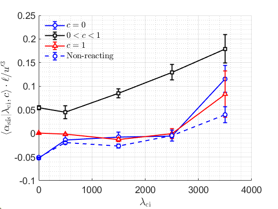
To further articulate the simultaneous effects of the flame and eddies on $\alpha_{\mathrm{sfs}}$, Fig.  6(b) shows the conditional mean $\langle\alpha_{\mathrm{sfs}}|{\lambda_{\mathrm{ci}}},c\rangle$ for both the reacting and non-reacting flows (the PDFs in Fig. 6(a) are from the data comprising the mean at $\lambda_{\mathrm{ci}}=1500$ in Fig.  6(b)). The error bars indicate the expected uncertainty in the mean based on the sample standard deviation and number of samples, approximating the statistics as normal. For the non-reacting case, $\langle\alpha_{\mathrm{sfs}}\rangle$ is negative for most values of $\lambda_{\mathrm{ci}}$, obtaining a slightly positive value at locations of high swirl. The data in the reactants and products of the reacting case are qualitatively similar to the non-reacting case. Most interesting are the data within the flame, which clearly demonstrate the flame-induced mean back-scatter and that the back-scatter magnitude increases with the local swirling strength. Regions of locally high swirling strength are expected to correspond to local increases in reaction rate due to flame wrinkling and increased scalar gradients. Hence, the data are indicative of a positive correlation between local heat release rate and back-scatter.

The above results demonstrate how the presence of swirling eddies and flame affect the local cross-scale kinetic energy transfer. We now isolate the impact of the single most dominant coherent structure on the energy dynamics, namely the periodic vortex identified from the POD (see Fig. 4). To do so, we examine the phase-averaged $\lambda_{\mathrm{ci}}$, $\alpha_{\mathrm{sfs}}$, and $c$ profiles generated using POD modes 1 and 2 in the reacting and non-reacting flows.

Phase averaging is performed based on Eq. 5, and we further condition on specific spatial regions of interest. To demonstrate this, Fig. 7 shows an instantaneous schematic of $\lambda_{\mathrm{ci}}$ and $c$ in phase 7, showing the location of the phase-averaged vortex ($\langle\lambda_{\mathrm{ci}}|\theta_{i}\rangle$ - red contour), the location of the instantaneous vortex ($\lambda_{\mathrm{ci}}$ - green contour), and the region occupied by the flame ($0<c<1$ - magenta contour). The “$\mathrm{flame}~\cap~\mathrm{vortex}$” region (shaded green) represents the region where the flame, $\lambda_{\mathrm{ci}}$, and $\langle\lambda_{\mathrm{ci}}|\theta_{i}\rangle$ intersect; the instantaneous vortex that lies outside the $\langle\lambda_{\mathrm{ci}}|\theta_{i}\rangle$ contour is not part of the periodic vortex and, hence, is not considered in this analysis. The “$\mathrm{flame}~\cap~\overline{\mathrm{vortex}}$” region (shaded purple) represents the locations inside the flame but external to the instantaneous vortex inside the $\langle\lambda_{\mathrm{ci}}|\theta_{i}\rangle$ contour. We also consider “$\mathrm{vortex}$” and “$\overline{\mathrm{vortex}}$” which represent overlapping regions of $\lambda_{\mathrm{ci}}$ and $\langle\lambda_{\mathrm{ci}}|\theta_{i}\rangle$ and its complement set, respectively. Finally, the “$\mathrm{reactants}$” region (shaded light blue) represents regions of $c=0$. We do not present data in the products (shaded orange), as $\alpha_{\mathrm{sfs}}$ generally is low in this region due to the attenuated turbulence.

Figure 8(a) shows the phase-averaged $\alpha_{\mathrm{sfs}}$ in different regions of the flow as a function of phase. In the reactants and in the non-reacting flow, $\langle\alpha_{\mathrm{sfs}}|\theta_{i}\rangle$ is negative and no significant phase dependence is observed. For the non-reacting flow, the increased scatter for regions containing the periodic vortex likely is attributed to uncertainty and convergence. Broadly speaking, the non-reacting flow and non-reacting regions of the reacting flow both show mean forward-scatter across the filter scale.

The regions containing the flame show qualitative differences in $\alpha_{\mathrm{sfs}}$ compared to the non-reacting flows, with further qualitative differences between regions with and without the dominant periodic vortex. In the “$\mathrm{flame}~\cap~\overline{\mathrm{vortex}}$” region, $\langle\alpha_{\mathrm{sfs}}|\theta_{i},\mathrm{flame}~\cap~\overline{\mathrm{vortex}}\rangle$ is positive. This is consistent with our previous experimental findings [5] and other DNS studies [2, 3, 4], demonstrating that the flame leads to mean back-scatter at scales around the laminar flame thickness. Importantly, regions where the flame and periodic vortex intersect exhibit higher mean back-scatter compared to regions of the flame without the vortex present, i.e. $\langle\alpha_{\mathrm{sfs}}|\theta_{i},\mathrm{flame}~\cap~{\mathrm{vortex}}\rangle>\langle\alpha_{\mathrm{sfs}}|\theta_{i},\mathrm{flame}~\cap~\overline{\mathrm{vortex}}\rangle$ .

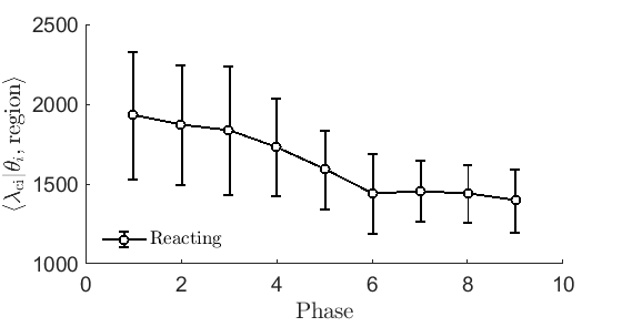
The magnitude of $\langle\alpha_{\mathrm{sfs}}|\theta_{i},\mathrm{flame}~\cap~{\mathrm{vortex}}\rangle$ decreases with phase. Figure 8(b) shows that the magnitude of the swirl, i.e. $\langle{\lambda_{\mathrm{ci}}}|\theta_{i},\mathrm{flame}~\cap~\mathrm{vortex}\rangle$, also decreases with phase as the vortex moves downstream. Hence, there is a correspondence between the swirling strength of the dominant periodic vortex and the mean back-scatter magnitude at locations of flame/vortex interaction. This result is consistent with the instantaneous data in Fig. 6(b) and further articulates the simultaneous and complimentary effects of combustion induced heat release rate and large-scale coherent vortices on kinetic energy back-scatter.

References

- [1] A. M. Steinberg, P. E. Hamlington, X. Zhao, Structure and Dynamics of Highly Turbulent Premixed Combustion, Prog. Energy Combust. Sci. (2020).
- [2] C. A. Z. Towery, A. Y. Poludnenko, J. Urzay, J. OBrien, M. Ihme, P. E. Hamlington, Spectral kinetic energy transfer in turbulent premixed reacting flows, Phys. Rev. E 93 (5) (5 2016).
- [3] J. O’Brien, C. A. Towery, P. E. Hamlington, M. Ihme, A. Y. Poludnenko, J. Urzay, The cross-scale physical-space transfer of kinetic energy in turbulent premixed flames, Proc. Combust. Inst. 36 (2) (2017) 1967–1975.
- [4] J. Kim, M. Bassenne, C. A. Z. Towery, P. E. Hamlington, A. Y. Poludnenko, J. Urzay, Spatially localized multi-scale energy transfer in turbulent premixed combustion, J. Fluid Mech. 848 (2018) 78–116.
- [5] A. Kazbekov, A. Steinberg, Physical space analysis of cross-scale turbulent kinetic energy transfer in premixed swirl flames, Combust. Flame 229 (2021).
- [6] J. F. MacArt, T. Grenga, M. E. Mueller, Effects of combustion heat release on velocity and scalar statistics in turbulent premixed jet flames at low and high Karlovitz numbers, Combust. Flame 191 (2018) 468–485.
- [7] M. Sieber, C. Oliver Paschereit, K. Oberleithner, Advanced Identification of Coherent Structures in Swirl-Stabilized Combustors, J. Eng. Gas Turbines Power 139 (2) (2 2017).
- [8] K. Oberleithner, M. Sieber, C. N. Nayeri, C. O. Paschereit, C. Petz, H.-C. Hege, B. R. Noack, I. Wygnanski, Three-dimensional coherent structures in a swirling jet undergoing vortex breakdown: stability analysis and empirical mode construction, J. Fluid Mech. 679 (2011) 383–414.
- [9] A. Steinberg, C. Arndt, W. Meier, Parametric study of vortex structures and their dynamics in swirl-stabilized combustion, Proc. Combust. Inst. 34 (2) (2013) 3117–3125.
- [10] S. Terhaar, T. G. Reichel, C. Schrödinger, L. Rukes, C. O. Paschereit, K. Oberleithner, Vortex Breakdown Types and Global Modes in Swirling Combustor Flows with Axial Injection, J. Propul. Power 31 (1) (2015) 219–229.
- [11] P. Holmes, J. L. Lumley, G. Berkooz, Turbulence, Coherent Structures, Dynamical Systems and Symmetry, Cambridge University Press, 1996.
- [12] J. Zhou, R. J. Adrian, S. Balachandar, T. M. Kendall, Mechanisms for generating coherent packets of hairpin vortices in channel flow, J. Fluid Mech. 387 (5 1999).
- [13] A. Kazbekov, K. Kumashiro, A. Steinberg, Enstrophy transport in swirl combustion 876 (2019).
- [14] A. Kazbekov, A. Steinberg, Flame- and flow-conditioned vorticity transport in premixed swirl combustion, Proc. Combust. Inst. (2020).
- [15] W. Meier, P. Weigand, X. Duan, R. Giezendanner-Thoben, Detailed characterization of the dynamics of thermoacoustic pulsations in a lean premixed swirl flame, Combust. Flame 150 (1-2) (2007) 2–26.
- [16] D. G. Goodwin, R. L. Speth, H. K. Moffat, B. W. Weber, Cantera: An Object-oriented Software Toolkit for Chemical Kinetics, Thermodynamics, and Transport Processes (2018).
- [17] J. Zhong, T. Huang, R. Adrian, Extracting 3D vortices in turbulent fluid flow, IEEE Trans. Pattern Anal. Mach. Intell. 20 (2) (1998).
- [18] V. Kolář, Vortex identification: New requirements and limitations, Int. J. Heat Fluid Flow 28 (4) (2007) 638–652.
- [19] L. Sirovich, Turbulence and the dynamics of coherent structures. I. Coherent structures, Q. Appl. Math. 45 (3) (1987) 561–571.
- [20] P. Gilge, J. R. Seume, K. Mulleners, Experimental Analysis of Multiscale Vortex Shedding in Turbulent Turbomachine Blade Wakes, AIAA Journal 58 (12) (2020) 5183–5190.
- [21] B. W. v. Oudheusden, F. Scarano, N. P. v. Hinsberg, D. W. Watt, Phase-resolved characterization of vortex shedding in the near wake of a square-section cylinder at incidence, Exp. Fluids 39 (1) (2005) 86–98.
- [22] R. Perrin, M. Braza, E. Cid, S. Cazin, A. Barthet, A. Sevrain, C. Mockett, F. Thiele, Obtaining phase averaged turbulence properties in the near wake of a circular cylinder at high Reynolds number using POD, Exp. Fluids 43 (2-3) (2007) 341–355.
- [23] M. Legrand, J. Nogueira, A. Lecuona, Flow temporal reconstruction from non-time-resolved data part I: mathematic fundamentals, Exp. Fluids 51 (4) (2011) 1047–1055.