Obstacles for dS in Supersymmetric Theories

Here we prove that de Sitter critical point in $\mathcal{N}=2$ supergravity with charged massless gravitini do not have parametric separation between the Hubble scale and the mWGC cutoff. Recall that the gravitino mass and charge matrices can be written as

	$\displaystyle S_{ij}$	$\displaystyle=iP^{x}_{\Lambda}L^{\Lambda}(\sigma_{x})_{i}^{k}\epsilon_{jk}$		(3)
	$\displaystyle(Q_{A})_{i}^{\ j}$	$\displaystyle=\frac{1}{2}\mathcal{E}^{\Lambda}_{A}\big(P^{0}_{\Lambda}\delta_{i}^{\ j}+P^{x}_{\Lambda}(\sigma^{x})_{i}^{\ j}\big)$

where $L^{\Lambda}$ denotes the choice of covariantly holomorphic section that specifies the scalar manifold for the vector multiplets and $P_{\Lambda}^{0,x}$ denote the prepotentials, which are computed from the killing vectors that specify the scalar manifold isometries gauged by the available vector fields. The “gauge vielbein" $\mathcal{E}^{\Lambda}_{A}$ defines the canonically normalized charges and is related to the gauge-kinetic matrix $\mathcal{I}$ by

$$\mathcal{E}_{A}^{\Lambda}\mathcal{E}_{B}^{\Sigma}\delta^{AB}=-\mathcal{I}^{-1|\Lambda\Sigma}$$

(4)

This means that the eigenvalues of $Q_{A}$ are the physical gravitino charges, which are to be used when applying the mWGC. Meanwhile, the scalar potential is a sum of three terms

$$\mathcal{V}=\mathcal{V}_{1}+\mathcal{V}_{2}+\mathcal{V}_{3}$$

(5)

with

	$\displaystyle\mathcal{V}_{1}$	$\displaystyle=g_{I\bar{J}}k^{I}_{\Lambda}k^{\bar{J}}_{\Sigma}\bar{L}^{\Lambda}L^{\Sigma}$		(6)
	$\displaystyle\mathcal{V}_{2}$	$\displaystyle=4h_{uv}k^{u}_{\Lambda}k^{v}_{\Sigma}L^{\Lambda}\bar{L}^{\Sigma}$
	$\displaystyle\mathcal{V}_{3}$	$\displaystyle=(U^{\Lambda\Sigma}-3L^{\Lambda}\bar{L}^{\Sigma})P^{x}_{\Lambda}P^{x}_{\Sigma}$

where $g_{IJ}$ is the metric on the scalar manifold for the vector multiplets, $h_{uv}$ is the metric on the scalar manifold of the hypermultiplets and $U^{\Lambda\Sigma}=g^{I\bar{J}}\nabla_{I}L^{\Lambda}\nabla_{\bar{J}}\bar{L}^{\Sigma}=-\frac{1}{2}(\mathcal{I}^{-1})^{\Lambda\Sigma}-\bar{L}^{\Lambda}L^{\Sigma}$. A vanishing mass matrix $S_{i}j$ requires $P^{x}_{\Lambda}L^{\Lambda}=0$. This simplifies the expression for the scalar potential to

$$\mathcal{V}=-\frac{1}{2}\mathcal{I}^{-1|\Lambda\Sigma}\big(P^{0}_{\Lambda}P^{0}_{\Sigma}+P^{x}_{\Lambda}P^{x}_{\Sigma}\big)+4h_{uv}k^{u}_{\Lambda}k^{v}_{\Sigma}L^{\Lambda}\bar{L}^{\Sigma}$$

(7)

where in the first term we used the relations between the killing vectors $k_{\Lambda}^{I}$, their corresponding prepotentials $P_{\Lambda}^{0}$, and the gauge-kinetic matrix to rewrite $\mathcal{V}_{1}$. $\mathcal{V}_{3}$ itself simplifies to a similar looking form, but involving the prepotentials associated to the hypermultiplet scalar manifold. The last term is simply $\mathcal{V}_{2}$ and is positive definite. Since we are interested in finding a lower bound on the scalar potential we can drop this term and write

$$\mathcal{V}\geq\frac{1}{2}\delta^{AB}\big(P^{0}_{A}P^{0}_{B}+P^{x}_{A}P^{x}_{B}\big)=\frac{1}{2}\delta^{AB}\big(\delta_{i}^{j}P_{A}^{0}+\sigma^{x}\ _{i}{}^{j}P_{A}^{x}\big)\big(\delta_{i}^{j}P_{B}^{0}+\sigma^{x}\ _{i}{}^{j}P_{B}^{x}\big)$$

(8)

where we traded the gauge indices $\Lambda,\Sigma$ for their “flat" counterparts $A,B$ using $\mathcal{E}_{\Lambda}^{A}$ that we introduced earlier. In the second equality, we re-expressed the sum over the $0,x$ in terms of the traces of products of Pauli matrices (along with the identity). We recognize the terms in the parentheses as the expressions for the gravitino charge matrix given in (3). In particular, we can choose $\mathcal{E}_{\Lambda}^{A}$ such that the $U(1)$ charge that we intend to use for the mWGC lies along the $A=1$ direction and we can thus write the lower bound

$$\mathcal{V}\geq\frac{1}{2}\text{Tr}(Q_{1}Q_{1})=q_{1}^{2}+q_{2}^{2}$$

(9)

where $q_{1}$ and $q_{2}$ are the physical charges of the individual gravitini, which themselves provide an upper bound on the UV cutoff from the mWGC $q_{1}^{2}+q_{2}^{2}\geq\Lambda_{UV}^{2}$. The final conclusion is that we have

$$\mathcal{V}\geq q_{1}^{2}+q_{2}^{2}\geq\Lambda_{UV}^{2}\implies H\geq\Lambda_{UV}/\sqrt{3}$$

(10)

Thus the Hubble scale associated to the value of the potential is bounded below by an energy of order the mWGC cutoff, invalidating the EFT description of such critical points. ¹¹ 1 An analogous proof for $\mathcal{N}=8$ supergravity was also given in [26]. One can reasonably expect that the result holds for all extended supergravity theories, but the full proof is currently unavailable.

A couple of remarks are in order here. First, the proof assumes that the full mass matrix vanishes, i.e. that both gravitini are massless. This assumption completely removes the negative contributions to the potential, allowing us to place the lower bounds in the way that we do. Second, the proof does not assume that we are precisely at a critical point of the potential, except for the last step where the Hubble scale is determined from the potential. This means that the conclusion should also be valid for quasi-de Sitter backgrounds, as long as the notion of a cosmological horizon and a corresponding Hubble scale makes sense. We will see both these considerations at play in the second example presented in the next subsection.

Finally an important note is that our result is contained within the “Festina-Lente" bound, which places a lower bound on the masses of all charged particles in a de Sitter background. This bound can be derived from considering the evaporation process of large black holes in de Sitter space and its connection to the Weak Gravity Conjecture has also been discussed [33, 34, 35]. It is a non-trivial cross check that at least a sub-statement of this bound can also be derived purely on mWGC grounds.

As an illustrative example of our result at work, as well as of its caveats and possible extensions we will present two very similar models, which have the same matter content, but differ in the gauging. A distinguishing feature of the first example is a flat direction that tunes the gravitino mass, interpolating between regions that respect or violate the mWGC. The second example has several critical points, which exhibit either non-abelian enhancement of the gauge group, or its complete breaking, both of which are obstacles to applying the mWGC. Additional examples with interesting properties can be found in [25, 26], including fully stable de Sitter critical points, whose EFT validity are however ruled out by the mWGC. Earlier works on finding de Sitter critical points in extended supergravity include [36, 37, 38]

The models we are going to consider will have the following scalar manifolds

$$\mathcal{M}_{SK}=\frac{\text{SU(1,3)}}{\text{SU(3)}\times\text{U(1)}}\ ,\qquad\mathcal{M}_{QK}=\frac{\text{SO(4,2)}}{\text{SO(4)}\times\text{SO(2)}}\,,$$

(11)

with holomorphic section

$$Z=\begin{pmatrix}1\\ z^{I}\\ -i/2\\ iz^{I}/2\end{pmatrix}\ ,\qquad I=1,2,3\ .$$

(12)

There is an $SO(3)$ isometry of $\mathcal{M}_{SK}$, which rotates the $z^{I}$ into each other, given by the killing vectors

$$\kappa_{1}^{I}=\begin{pmatrix}0\\ z_{3}\\ -z_{2}\end{pmatrix}\ ,\quad\kappa_{2}^{I}=\begin{pmatrix}-z_{3}\\ 0\\ z_{1}\end{pmatrix}\ ,\quad\kappa_{3}^{I}=\begin{pmatrix}z_{2}\\ -z_{1}\\ 0\end{pmatrix}$$

(13)

while $\mathcal{M}_{QK}$ has an $SO(3)$ isometry generated by $T_{\underline{12}},T_{\underline{13}},T_{\underline{23}}$, an $O(1,1)$ generated by $T_{\underline{46}}$ and a $U(1)$ isometry generated by $T_{\underline{56}}$, where

$$(T_{\underline{ab}})_{\underline{c}}{}^{\underline{d}}=\eta_{\underline{c}[\underline{a}}\delta_{\underline{b}]}^{\underline{d}}$$

(14)

are the $SO(4,2)$ generators used in the construction of $\mathcal{M}_{QK}$.

The $\mathcal{M}_{SK}$ isometries are gauged by the three vector multiplets as

$$k_{\Lambda}^{I}=e_{1}\,\big(0\ ,\ \kappa_{1}^{I}\ ,\ \kappa_{2}^{I}\ ,\ \kappa_{3}^{I}\big)\,.$$

(15)

and the SO(3)$\times$O(1,1) isometry of $\mathcal{M}_{QK}$ are gauged as

$\displaystyle k_{\Lambda}^{u}=\big(e_{0}k_{T_{\underline{46}}}^{u}\ ,\ e_{1}k_{T_{\underline{12}}}^{u}\ ,\ e_{1}k_{T_{\underline{13}}}^{u}\ ,\ e_{1}k_{T_{\underline{23}}}^{u}\big).$

(16)

i.e. the $SO(3)$ isometry is still gauged by the three vector multiplets, with the same charge $e_{1}$ as the $\mathcal{M}_{SK}$ isometries, while the $O(1,1)$ is gauged by the graviphoton with charge $e_{0}$. The corresponding prepotentials given by

$\displaystyle P_{0}^{x}=\begin{pmatrix}0\\ 0\\ 0\end{pmatrix}\ ,\quad P_{1}^{x}=\begin{pmatrix}e_{1}\\ 0\\ 0\end{pmatrix}\ ,\quad P_{2}^{x}=\begin{pmatrix}0\\ e_{1}\\ 0\end{pmatrix}\ ,\quad P_{3}^{x}=\begin{pmatrix}0\\ 0\\ e_{1}\end{pmatrix}\ ,$

(17)

The resulting scalar potential has a critical point at the center of field space with

$\displaystyle{\cal V}=2\,e_{0}^{2}+3\,e_{1}^{2}$

(18)

and scalar masses related to the value of the potential as

$\displaystyle\begin{split}m^{2}_{(mult.)}&=\left(0_{(1)}\ ,\ 2(e_{0}^{2}-e_{1}^{2})_{(3)}\ ,\ 4e^{2}_{0\ (1)}\ ,\ 4e^{2}_{1\ (2)}\right.\ ,\\ &\quad x_{1\ {(1)}}\ ,\ x_{2\ {(1)}}\ ,\ x_{3\ {(1)}}\\[5.69054pt] &\quad e_{1}^{2}+\sqrt{4e_{0}^{4}-4e_{0}^{2}e_{1}^{2}+9e_{1}^{4}}_{(2)}\ ,\\ &\left.\ e_{1}^{2}-\sqrt{4e_{0}^{4}-4e_{0}^{2}e_{1}^{2}+9e_{1}^{4}}_{(2)}\right)\times{\cal V}\,\end{split}$

(19)

where $x_{1},x_{2},x_{3}$ are the solutions to

$$x^{3}+6e_{1}x^{2}+(4e_{0}^{2}e_{1}^{2}-4e_{0}^{4})x-(16e_{0}^{4}e_{1}^{2}-16e_{0}^{2}e_{1}^{4}+32e_{1}^{6})=0$$

(20)

Note that the critical point is unstable and its mass spectrum marginally respects the de Sitter conjecture. If we further choose $e_{0}=e_{1}$ the scalar potential develops a flat direction along the imaginary directions of each of the $z^{I}$. Moving along any one of these flat directions will break the $SO(3)$ isometry to a $U(1)$, with the corresponding gravitino charge given by

$$q_{U(1)}=\pm\sqrt{\frac{1+z^{2}}{1-z^{2}}}$$

(21)

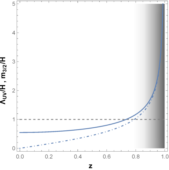
where $z$ is the magnitude of the imaginary part of the scalar that parametrizes our chosen flat direction. This $U(1)$ physical charge, and therefore the mWGC cutoff, interpolates between $1$ and infinity as $z$ grows from $0$ to $1$. Meanwhile, the gravitino mass along this direction is given by

$$S_{ij}=\begin{pmatrix}e_{1}\frac{z}{\sqrt{1-z^{2}}}&0\\ 0&e_{1}\frac{z}{\sqrt{1-z^{2}}}\end{pmatrix}$$

(22)

which vanishes as $z\to 0$ and diverges as $z\to 1$. This flat direction thus offers a perfect opportunity to illustrate the onset of the mWGC violation as we approach the massless point. Indeed, computing the mWGC cutoff in units of the Hubble scale as a function of $z$ we can see that the well-controlled regime appears precisely as $z\to 1$, where the gravitini are heavy, while the massless gravitino limit has the Hubble scale on the same order as the mWGC cutoff (see Figure 1).

Finally we also note that at $z=0$ the unbroken gauge symmetry gets enhanced to $SO(3)$, which is non-abelian and so the mWGC does not directly apply. However, since points along the flat directions are excluded by the mWGC arbitrarily close to the central critical point, we may conclude by continuity that the central point is similarly excluded.

As our second example, we may choose instead to gauge the $U(1)$ isometry on $\mathcal{M}_{QK}$ instead of the $O(1,1)$, i.e. choose

$\displaystyle k_{\Lambda}^{u}=\big(e_{0}k_{T_{\underline{56}}}^{u}\ ,\ e_{1}k_{T_{\underline{12}}}^{u}\ ,\ e_{1}k_{T_{\underline{13}}}^{u}\ ,\ e_{1}k_{T_{\underline{23}}}^{u}\big).$

(23)

with the rest of the model exactly as before. In particular the prepotentials are still given by (17). With this choice of gauging, the central critical point still exists and has energy

$$\mathcal{V}=3e_{1}^{2}$$

(24)

with the mass spectrum

$$m^{2}_{(mult.)}=\left(-\frac{2}{3}_{(6)}\ ,\ \frac{4}{3}r^{2}_{(2)}\ ,\ \frac{4}{3}(r^{2}+1)_{(6)}\right)\times{\cal V}$$

(25)

The vanishing of $P^{x}_{0}$ implies that the gravitini are uncharged under the separate $U(1)$ isometry. They do have charges $\pm\frac{1}{\sqrt{2}}e_{1}$ under the three generators of the $SO(3)$ isometry. However this isometry is non-abelian, so it isn’t clear that the mWGC constraint can be applied. Furthermore, we no longer have the flat direction that allows us to break it to a single $U(1)$.

A possible way around this problem is to consider time-dependent trajectories, which have as initial boundary conditions points near, but not quite at, the central critical point, in such a way that the $SO(3)$ symmetry is broken down to $U(1)$ as in the previous example. In this case, the charge under this $U(1)$ will still be approximately equal to $\pm\frac{1}{\sqrt{2}}e_{1}$ and the energy, at least for some short time before the runaway due to the tachyonic directions takes over, will be above the mWGC cutoff, so we expect the EFT description around these trajectories to break down. By considering a limit of such runaway trajectories such that their initial conditions approach the critical point, we might wish to again conclude by continuity that the critical point itself also suffers a breakdown of its EFT description.

An important caveat to the above argument is that since the masses of the tachyons are comparable to the energy itself and therefore does not satisfy slow-roll conditions, it isn’t clear that the mWGC criterion applies to such trajectories in the first place, since one can not meaningfully assign a Hubble radius to this solution. This question deserves further investigation.

Finally, a second interesting feature of this model is the presence of a second family of critical points located at

$$\text{Re}\,z_{I}=\pm\frac{1}{2}\ ,\ \text{Im}\,z_{J}=\pm\frac{1}{2}\,I\neq J\ .$$

(26)

This critical point completely breaks the $SO(3)$ gauge symmetry, and the gravitino $U(1)$ charge continutes to vanish. The scalar mass spectrum is

$\displaystyle m^{2}_{(mult.)}$

$\displaystyle=\left(0_{(3)},-1_{(2)},8_{(1)},2+4r^{2}-2r_{(2)},\beta^{2}+\beta_{(2)},\beta^{2}-\beta_{(2)},2+2r+4r^{2}_{(2)}\right)\times{\cal V}\,$

(27)

and thus again has tachyons satisfying the de Sitter criterion. This critical point can therefore not be excluded by this criterion, nor by the mWGC due to a lack of any unbroken gauge group. The reason this is not a counterexample to our general theorem is that one of the gravitini becomes massive. Indeed the mass matrix evaluated at this critical point is

$$S_{ij}=\begin{pmatrix}\sqrt{2}\,e_{1}&0\\ 0&0\end{pmatrix}\,$$

(28)

illustrating that insufficiency of having a single massless gravitino to exclude a critical point on mWGC grounds.

Our starting point is the Volkov-Akulov model [39], which is a theory of a single goldstone fermion with Lagrangian

$\displaystyle{\cal L}=-f^{2}+iG\sigma^{m}\partial_{m}\overline{G}-\frac{1}{4f^{2}}\overline{G}^{2}\partial^{2}G^{2}-\frac{1}{16f^{6}}G^{2}\overline{G}^{2}\partial^{2}G^{2}\partial^{2}\overline{G}^{2}$

(29)

The higher derivative terms are required by supersymmetry, which is realized non-linearly, with the supersymmetry transformation taking the form $\delta_{\epsilon}G=-\sqrt{2}f\epsilon+...$.

This model appears, at least as a sub-sector, in the low-energy description of theories with spontaneous supersymmetry breaking. The supersymmetry breaking scale is given by $\sqrt{f}$. The model can alternatively be written in superspace by means of a nilpotent chiral superfield [13, 14]

$\displaystyle X=\phi+\sqrt{2}\theta G+\theta^{2}F\ ,\ X^{2}=0\implies\phi=\frac{G^{2}}{2F}$

(30)

with Lagrangian given by

	$\displaystyle L$	$\displaystyle=\int d^{4}\theta K(X,\overline{X})+\bigg(\int d^{2}\theta W(X)+c.c\bigg)$		(31)
		$\displaystyle=\int d^{4}\theta|X|^{2}+\left(\int d^{2}\theta fX+\text{c.c.}\right)$

or equivalently, one can impose the nilpotency condition via a second non-dynamical chiral superfield $T=\tau+\sqrt{2}\theta\lambda+\theta^{2}B$ that acts as a lagrange multipler

$\displaystyle L$

$\displaystyle=\int d^{4}\theta|X|^{2}+\left(\int d^{2}\theta fX+TX^{2}+\text{c.c.}\right)$

(32)

Despite appearing to have additional fields, the scalar fields $\phi,\tau$ as well as the fermion $\lambda$ are all non-dynamical and can be written as an expansion in goldstino multilinears as

$\displaystyle\langle\phi\rangle\ \sim\ \Big\langle\frac{G^{2}}{f}\Big\rangle+\dots\ ,\quad\langle\tau\rangle\ \sim\ \Big\langle\frac{\partial^{2}\overline{G}^{2}}{f^{2}}\Big\rangle+\dots{}$

(33)

and $\lambda$ can be determined by acting with a supersymmetry transformation on $\tau$. Thus the goldstino is still the unique independent degree of freedom in the theory.

The presence of goldstino self-interactions presents the possibility that besides the perturbative goldstino states, composite states might also appear in the theory, represented precisely by expressions such as those for $\phi$ and $\tau$ above. One way to determine whether this happens is to allow the theory to evolve along the Wilsonian RG flow and see whether the non-dynamical field $\tau$ acquires a correct-sign kinetic term, similar to Nambu–Jona-Lasinio and composite Higgs models [40, 41, 42]. In this case, not only would a kinetic term indicate that $\tau$ itself represents dynamical states, but also the nilpotency condition on $X$ would get relaxed and so $\phi$ would also enter the theory as an independent degree of freedom. The behavior of these new composite states will then be governed by the resulting scalar potential for $\phi$ and $\tau$.

Since the $T$ superfield starts out with a vanishing kinetic term, small variations of the Wilsonian cutoff will produce a small kinetic term, which is equivalent to strong coupling. We can therefore not rely on any perturbative calculation in the couplings and must turn to the formalism of the Exact Renormalization Group [43, 44, 45].

The main idea behind this formalism is that given a Wilsonian effective action $L[\Phi;\mu]$ with cutoff $\mu$, the partition function

	$\displaystyle\mathcal{Z}[\Phi]$	$\displaystyle=\int\mathcal{D}\Phi\ e^{L_{\text{prop.}}[\Phi;\mu]+L_{\text{int.}}[\Phi;\mu]}$		(34)
	$\displaystyle L_{\text{prop.}}[\Phi;\mu]$	$\displaystyle=\int\frac{d^{4}k}{(2\pi)^{4}}\Phi^{A}(-k)C_{AB}^{-1}(k)\Phi^{B}(k)$
	$\displaystyle L_{\text{int.}}[\Phi;\mu]$	$\displaystyle=\int\sum_{\lambda}g_{\lambda}(\mu)\prod_{\{A\}_{\lambda}}\bigg(\frac{d^{4}k_{A}}{(2\pi)^{4}}k_{A}^{n_{A,\lambda}}\Phi^{A}(k_{A})\bigg)\delta(\sum_{\{A\}_{\lambda}}k_{A})$

should be independent of $\mu$. Here we separated the action into a regularized propagator piece $L_{\text{prop.}}$, which needs not include the full kinetic term, and an interaction piece $L_{\text{int.}}$, which can still have term quadratic in the field. All fields, couplings and momenta are taken here to be rendered dimensionless by rescaling with appropriate powers of $\mu$.

The requirement of invariance of the partition function leads to the condition [43]

	$\displaystyle\dot{L}_{\text{int.}}$	$\displaystyle\equiv-\mu\partial_{\mu}L_{\text{int.}}$		(35)
		$\displaystyle=\int\frac{d^{4}k}{(2\pi)^{4}}\tilde{C}^{AB}(k)\bigg(\frac{\delta^{2}L_{\text{int.}}}{\delta\Phi^{A}(-k)\delta\Phi^{B}(k)}+\frac{\delta L_{\text{int.}}}{\delta\Phi^{A}(-k)}\frac{\delta L_{\text{int.}}}{\delta\Phi^{B}(k)}\bigg)$

where $\tilde{C}^{AB}$ is related to $C^{AB}$ in a specified way that depends on the spin of the field. It is worth emphasizing that this flow equation does not make use of any small-coupling approximation. It does however produce an infinite system of equations for all the higher derivative couplings that will generically be generated by the RG flow. Solving these equations thus requires an appropriate choice of truncation of these equations, typically based on a derivative expansion.

For our case, we resort to a truncation of the equations that we dub the Supersymmetric Local Potential Approximation (SLPA). In this approximation we ignore all contributions to and from any terms that can not be expressed in terms of a Kähler or superpotential. In superspace, this amounts to ignoring all terms that are higher-order in superderivatives. The SLPA has the benefit of preserving supersymmetry (assuming a supersymmetric regulator function) and keeping track of the kinetic terms of the scalar fields, which is what we are interested in. This is in contrast to the more common Local Potential Approximation (LPA) which would simply truncate all derivative interactions [46, 47, 48, 49].

The truncation of higher order terms means that we should not trust the solutions to the remaining equations for large changes in $\mu$. This can be an issue when the qualitative features one is after do not appear immediately in the RG flow, such as the tachyonic behavior in composite Higgs models [42]. As we will see, the features describing here will not suffer from this problem, and will be immediately visible even for a small decrease in $\mu$.

In order to apply the ERG formalism to the Volkov–Akulov model, we start with the following Kähler and superpotentials

	$\displaystyle K$	$\displaystyle=\alpha|X|^{2}+\beta|T|^{2}+g\,|T|^{2}|X|^{2}+\frac{1}{4}q\,|X|^{4}$		(36)
	$\displaystyle W$	$\displaystyle=fX+\frac{1}{2}TX^{2}$

and separate $K$ into a (regularized) propagator and interaction part

	$\displaystyle K_{\text{prop.}}$	$\displaystyle=c^{-1}|X|^{2}+c^{-1}|T|^{2}$		(37)
	$\displaystyle K_{\text{int.}}$	$\displaystyle=(\alpha-1)|X|^{2}+(\beta-1)|T|^{2}+\gamma\mu^{-2}|T|^{2}|X|^{2}+\frac{1}{4}\zeta\mu^{-2}|X|^{4}$

where we assume the regulator function can be expanded as $c(p^{2}/\mu^{2})=1+\sum c_{n}\ p^{2n}/\mu^{2n}$. This action contains all the terms that will be generated by the RG flow within the SLPA. Since the action is manifestly supersymmetric, we can read off the flow of the couplings $\alpha,\beta,\gamma$ and $\zeta$ from any of the terms that contain them. A convenient choice are the quadratic terms in the auxiliary fields $F$ and $B$. The calculation is laborious but straightforward and can be found in full detail in [27]. Here we simply quote the resulting flow equations

	$\displaystyle\dot{\zeta}$	$\displaystyle=-2\zeta-2c_{1}\,,\quad\dot{\gamma}=-2\gamma-2c_{1}\,$		(38)
	$\displaystyle\dot{\beta}$	$\displaystyle=-2N\gamma\,,\quad\dot{\alpha}=-2N(\gamma+\zeta)\ ,$

The flow of the 4-point couplings $\zeta$ and $\gamma$ is generated by the second term in (35) from the $TX^{2}$ term in the superpotential. Once these terms are generated, the first term in (35) generates corrections to the kinetic terms from these 4-point couplings.

We now need to solve the Volkov–Akulov ERG equations with boundary conditions

$$\alpha\Big|_{t=0}=1\,,\quad\beta\Big|_{t=0}=0\,,\quad\gamma\Big|_{t=0}=0\,,\quad\zeta\Big|_{t=0}=0\,$$

(39)

with $t=\log(\Lambda/\mu)$, where $\Lambda\leq\sqrt{f}$ is a matching UV scale where we might imagine all other degrees of freedom are integrated out. $N$ is the result of a momentum loop integral that appears in the evaluation of the first term in (35) and $c_{1}$ is the first coefficient in the expansion of the regulator function. A typical monotonic regulator will have $c_{1}<0$ and $N<0$. The solution to this system of ODE’s is

	$\displaystyle\zeta$	$\displaystyle=-c_{1}\left(1-e^{-2t}\right)\,,\quad\gamma=-c_{1}\left(1-e^{-2t}\right)\,,$		(40)
	$\displaystyle\alpha$	$\displaystyle=1-2c_{1}N+4c_{1}N\left(t+\frac{1}{2}e^{-2t}\right)\,,$
	$\displaystyle\beta$	$\displaystyle=-c_{1}N+2c_{1}N\left(t+\frac{1}{2}e^{-2t}\right)>0\ .\,$

The $T$ field, which started its life as a Lagrange multiplier, acquires a positive kinetic term, indicating that the composite states of the goldstino that it represents enter the effective theory as independent degrees of freedom. Furthermore, we can evaluate the mass spectrum around the original Volkov–Akulov point at $X=T=0$ and we find that the masses take the form

$\displaystyle m_{\pm}^{2}=-\tilde{f}^{2}\left[\left(\tilde{\gamma}+4\tilde{\zeta}\right)\pm\sqrt{\frac{16\ \tilde{g}^{2}}{\tilde{f}^{2}}+\left(\tilde{\gamma}-4\tilde{\zeta}\right)^{2}}\ \right]\,.$

(41)

where $\tilde{f},\tilde{\gamma},\tilde{\zeta},\tilde{g}$ are rescaled couplings obtained after canonically normalizing the kinetic terms and are all positive. It isn’t hard to see that at least one of the masses is always negative and thus at least one of the scalars will develop an expectation value, representing the formation of a goldstino condensate. The typical behavior of the scalar potential for small $t$ is depicted in the left side of Figure 2.

For larger $t$ contributions beyond the SLPA will alter the flow from that given by (40). In particular additional couplings will enter the Kähler potential and affect the shape of the potential away from the central point. This may ultimately affect the endpoint of the instability and its physical interpretation. The central instability, however, is expected to survive, since both the generation of the kinetic term for $T$ and the tachyonic behavior at the origin is due to the $TX^{2}$ term in the superpotential. To remove the central instability, the effect of the higher-derivative contributions in the ERG flow would have to give corrections to the Kähler potential that compete with the effect of the superpotential term, which would indicate a breakdown of the EFT description altogether. While this is not ruled out, it would require an even bigger revision of what is commonly assumed about the IR behavior of the Volkov–Akulov model. In either case, an analysis beyond the SLPA is called for.

So far we have only considered the pure Volkov–Akulov model without additional fields and in the rigid limit. Additional fields are unlikely to change the qualitative features found above. This is, again, due to the fact that the $TX^{2}$ term in the superpotential is responsible for both the kinetic term of $T$ and for the presence of the central tachyon. At the UV matching scale, $T$ only appears in that single superpotential term and can not couple to any other fields in any larger model. The SLPA calculation for the kinetic term will therefor be unaffected. Beyond the SLPA, additional fields may have an effect and considerations of the previous paragraph apply. Once again, analysis to higher orders remains a necessary future direction.

As far as extending this analysis to supergravity, a major obstacle is the absence of a supersymmetric regulator, which could be used to maintain a manifestly supersymmetric RG flow. This remains an open problem. That said, the natural expectation is that corrections to the rigid limit results will be suppressed by powers of $M_{p}$ and so the main qualitative features of a dynamic $T$ and a tachyonic critical point should remain. As a naive first check, one can simply embed the RG-evolved V–A model into the KKLT scenario by adding the RG-evolved Kähler and superpotentials (36) evaluated at small $t$ to the pre-uplift KKLT Kähler and superpotentials. The details of this calculation are also described in [27] and the result is depicted in the right side of Figure 2. The main result is that the dS critical point shifts in the $X,T$- plane and also develops a tachyonic instability toward goldstino condensation. Of course one can look at more complicated models where the goldstino sector couples to other matter fields in more sophisticated ways, such as [22, 50, 51, 52], but the instability of the original critical point toward goldstino condensation is expected to remain for the reasons outlined above.

Finally, we note that since the Volkov–Akulov model is generally understood to be contained in the low-energy description of the worldvolume dynamics of anti-branes, the instability we find should be present in the simple case of the $\overline{D3}/O3$ system in 10 dimensions. In this context, a string theoretic analysis of the goldstino composite states and their dynamics could give insights into the eventual fate of the instability that would be difficult to access using effective field theory methods.

References

- [1] U. H. Danielsson and T. Van Riet, Int. J. Mod. Phys. D 27 (2018) no.12, 1830007 doi:10.1142/S0218271818300070 [arXiv:1804.01120 [hep-th]].
- [2] I. Antoniadis, E. Dudas and A. Sagnotti, Phys. Lett. B 464 (1999), 38-45 doi:10.1016/S0370-2693(99)01023-0 [arXiv:hep-th/9908023 [hep-th]].
- [3] J. Mourad and A. Sagnotti, [arXiv:1711.11494 [hep-th]].
- [4] J. Polchinski and A. Strominger, Phys. Lett. B 388 (1996), 736-742 doi:10.1016/S0370-2693(96)01219-1 [arXiv:hep-th/9510227 [hep-th]].
- [5] J. Michelson, Nucl. Phys. B 495 (1997), 127-148 doi:10.1016/S0550-3213(97)00184-3 [arXiv:hep-th/9610151 [hep-th]].
- [6] T. R. Taylor and C. Vafa, Phys. Lett. B 474 (2000), 130-137 doi:10.1016/S0370-2693(00)00005-8 [arXiv:hep-th/9912152 [hep-th]].
- [7] S. Gukov, C. Vafa and E. Witten, Nucl. Phys. B 584 (2000), 69-108 [erratum: Nucl. Phys. B 608 (2001), 477-478] doi:10.1016/S0550-3213(00)00373-4 [arXiv:hep-th/9906070 [hep-th]].
- [8] E. Witten, Nucl. Phys. B 474 (1996), 343-360 doi:10.1016/0550-3213(96)00283-0 [arXiv:hep-th/9604030 [hep-th]].
- [9] U. Lindstrom and M. Rocek, “CONSTRAINED LOCAL SUPERFIELDS”, Phys. Rev. D 19 (1979), 2300-2303
- [10] A. A. Kapustnikov, “NONLINEAR REALIZATION OF EINSTEINIAN SUPERGRAVITY”, Theor. Math. Phys. 47 (1981), 406-413
- [11] S. Samuel and J. Wess, “A Superfield Formulation of the Nonlinear Realization of Supersymmetry and Its Coupling to Supergravity”, Nucl. Phys. B 221 (1983), 153-177
- [12] E. A. Bergshoeff, D. Z. Freedman, R. Kallosh and A. Van Proeyen, “Pure de Sitter Supergravity”, Phys. Rev. D 92 (2015) no.8, 085040 [erratum: Phys. Rev. D 93 (2016) no.6, 069901] [arXiv:1507.08264 [hep-th]].
- [13] N. Cribiori, G. Dall’Agata and F. Farakos, “From Linear to Non-linear SUSY and Back Again”, JHEP 08 (2017), 117 [arXiv:1704.07387 [hep-th]].
- [14] G. Dall’Agata, E. Dudas and F. Farakos, “On the origin of constrained superfields”, JHEP 05 (2016), 041 [arXiv:1603.03416 [hep-th]].
- [15] S. Ferrara, R. Kallosh and A. Linde, “Cosmology with Nilpotent Superfields”, JHEP 10 (2014), 143 [arXiv:1408.4096 [hep-th]].
- [16] E. A. Bergshoeff, K. Dasgupta, R. Kallosh, A. Van Proeyen and T. Wrase, “ and dS”, JHEP 05 (2015), 058 [arXiv:1502.07627 [hep-th]].
- [17] I. Bandos, L. Martucci, D. Sorokin and M. Tonin, “Brane induced supersymmetry breaking and de Sitter supergravity”, JHEP 02 (2016), 080 [arXiv:1511.03024 [hep-th]].
- [18] K. Dasgupta, M. Emelin and E. McDonough, “Fermions on the antibrane: Higher order interactions and spontaneously broken supersymmetry”, Phys. Rev. D 95 (2017) no.2, 026003 [arXiv:1601.03409 [hep-th]].
- [19] N. Cribiori, R. Kallosh, C. Roupec and T. Wrase, “Uplifting Anti-D6-brane”, JHEP 12 (2019), 171 [arXiv:1909.08629 [hep-th]].
- [20] N. Cribiori, C. Roupec, M. Tournoy, A. Van Proeyen and T. Wrase, “Non-supersymmetric branes”, JHEP 07 (2020), 189 [arXiv:2004.13110 [hep-th]].
- [21] S. Kachru, R. Kallosh, A. D. Linde and S. P. Trivedi, “De Sitter vacua in string theory”, Phys. Rev. D 68 (2003), 046005 [arXiv:hep-th/0301240 [hep-th]].
- [22] S. Kachru, R. Kallosh, A. D. Linde, J. M. Maldacena, L. P. McAllister and S. P. Trivedi, JCAP 10 (2003), 013 doi:10.1088/1475-7516/2003/10/013 [arXiv:hep-th/0308055 [hep-th]].
- [23] V. Balasubramanian, P. Berglund, J. P. Conlon and F. Quevedo, “Systematics of moduli stabilisation in Calabi-Yau flux compactifications”, JHEP 03 (2005), 007 [arXiv:hep-th/0502058 [hep-th]].
- [24] I. Bena, E. Dudas, M. Graña, G. L. Monaco and D. Toulikas, “Bare-Bones de Sitter”, [arXiv:2202.02327 [hep-th]].
- [25] N. Cribiori, G. Dall’agata and F. Farakos, “Weak gravity versus de Sitter,” JHEP 04 (2021), 046 [arXiv:2011.06597 [hep-th]].
- [26] G. Dall’Agata, M. Emelin, F. Farakos and M. Morittu, “The unbearable lightness of charged gravitini,” JHEP 10 (2021), 076 [arXiv:2108.04254 [hep-th]].
- [27] G. Dall’Agata, M. Emelin, F. Farakos and M. Morittu, “Anti-brane uplift instability from goldstino condensation,” [arXiv:2203.12636 [hep-th]].
- [28] N. Arkani-Hamed, L. Motl, A. Nicolis and C. Vafa, “The String landscape, black holes and gravity as the weakest force,” JHEP 06 (2007), 060 [arXiv:hep-th/0601001 [hep-th]].
- [29] N. Cribiori, D. Lust and M. Scalisi, “The gravitino and the swampland,” JHEP 06 (2021), 071 [arXiv:2104.08288 [hep-th]].
- [30] A. Castellano, A. Font, A. Herraez and L. E. Ibáñez, “A Gravitino Distance Conjecture,” [arXiv:2104.10181 [hep-th]].
- [31] H. Ooguri and C. Vafa, Nucl. Phys. B 766 (2007), 21-33 doi:10.1016/j.nuclphysb.2006.10.033 [arXiv:hep-th/0605264 [hep-th]].
- [32] N. Cribiori, [arXiv:2203.15449 [hep-th]].
- [33] M. Montero, T. Van Riet and G. Venken, “Festina Lente: EFT Constraints from Charged Black Hole Evaporation in de Sitter,” JHEP 01 (2020), 039 [arXiv: 1910.01648 [hep-th]].
- [34] M. Montero, T. Van Riet and G. Venken, “A dS obstruction and its phenomenological consequences,” JHEP 05 (2020), 114 [arXiv:2001.11023 [hep-th]].
- [35] M. Montero, C. Vafa, T. Van Riet and G. Venken, “The FL bound and its phenomenological implications,” [arXiv:2106.07650 [hep-th]].
- [36] P. Fre, M. Trigiante and A. Van Proeyen, “Stable de Sitter vacua from N=2 supergravity,” Class. Quant. Grav. 19 (2002), 4167-4194 [arXiv:hep-th/0205119 [hep-th]].
- [37] G. Dall’Agata and G. Inverso, “de Sitter vacua in N = 8 supergravity and slow-roll conditions,” Phys. Lett. B 718 (2013), 1132-1136 [arXiv:1211.3414 [hep-th]].
- [38] F. Catino, C. A. Scrucca and P. Smyth, “Simple metastable de Sitter vacua in N=2 gauged supergravity”, [arXiv: 1302.1754 [hep-th]].
- [39] D. V. Volkov and V. P. Akulov, “Is the Neutrino a Goldstone Particle?”, Phys. Lett. B 46 (1973), 109-110.
- [40] Y. Nambu and G. Jona-Lasinio, “Dynamical Model of Elementary Particles Based on an Analogy with Superconductivity. 1.”, Phys. Rev. 122 (1961), 345-358
- [41] Y. Nambu and G. Jona-Lasinio, “DYNAMICAL MODEL OF ELEMENTARY PARTICLES BASED ON AN ANALOGY WITH SUPERCONDUCTIVITY. II”, Phys. Rev. 124 (1961), 246-254
- [42] W. A. Bardeen, C. T. Hill and M. Lindner, “Minimal Dynamical Symmetry Breaking of the Standard Model,” Phys. Rev. D 41 (1990), 1647
- [43] J. Polchinski, “Renormalization and Effective Lagrangians”, Nucl. Phys. B 231 (1984), 269-295.
- [44] R. D. Ball and R. S. Thorne, “Renormalizability of effective scalar field theory”, Annals Phys. 236 (1994), 117-204 [arXiv: hep-th/9310042 [hep-th]].
- [45] D. F. Litim and M. J. Trott, “Asymptotic safety of scalar field theories”, Phys. Rev. D 98 (2018) no.12, 125006 [arXiv: 1810.01678 [hep-th]].
- [46] G. Zumbach, “The Renormalization group in the local potential approximation and its applications to the O(n) model”, Nucl. Phys. B 413 (1994), 754-770
- [47] G. Zumbach, “The Local potential approximation of the renormalization group and its applications”, Phys. Lett. A 190 (1994), 225-230
- [48] T. R. Morris, “Derivative expansion of the exact renormalization group”, Phys. Lett. B 329 (1994), 241-248 [arXiv:hep-ph/9403340 [hep-ph]].
- [49] C. S. F. Harvey-Fros, “The Local potential approximation of the renormalization group”, [arXiv:hep-th/0108018 [hep-th]].
- [50] I. Bena, E. Dudas, M. Graña and S. Lüst, “Uplifting Runaways”, Fortsch. Phys. 67 (2019) no.1-2, 1800100 [arXiv:1809.06861 [hep-th]].
- [51] E. Dudas and S. Lüst, “An update on moduli stabilization with antibrane uplift”, JHEP 03 (2021), 107 [arXiv:1912.09948 [hep-th]].
- [52] B. V. Bento, D. Chakraborty, S. L. Parameswaran and I. Zavala, “A new de Sitter solution with a weakly warped deformed conifold”, JHEP 12 (2021), 124 [arXiv:2105.03370 [hep-th]].