Learning from Stochastically Revealed Preference
‡ Imperial College Business School, Imperial College London, xiaocheng.li@imperial.ac.uk
◇ Institute for Computational and Mathematical Engineering, Stanford University, chunlin@stanford.edu
Abstract
We study the learning problem of revealed preference in a stochastic setting: a learner observes the utility-maximizing actions of a set of agents whose utility follows some unknown distribution, and the learner aims to infer the distribution through the observations of actions. The problem can be viewed as a single-constraint special case of the inverse linear optimization problem. Existing works all assume that all the agents share one common utility which can easily be violated under practical contexts. In this paper, we consider two settings for the underlying utility distribution: a Gaussian setting where the customer utility follows the von Mises-Fisher distribution, and a -corruption setting where the customer utility distribution concentrates on one fixed vector with high probability and is arbitrarily corrupted otherwise. We devise Bayesian approaches for parameter estimation and develop theoretical guarantees for the recovery of the true parameter. We illustrate the algorithm performance through numerical experiments.
1 Introduction
The problem of learning from revealed preference refers to the learning of a common utility function for a set of agents based on the observations of the utility-maximizing actions from the agents. The revealed preference problem has a long history in economics (Samuelson 1948; Afriat 1967) (See (Varian 2006) for a review). A line of works (Beigman and Vohra 2006; Zadimoghaddam and Roth 2012; Balcan et al. 2014; Amin et al. 2015) formulate the problem as a learning problem with two objectives: (i) rationalizing a set of observations, i.e., to find a utility function which explains a set of past observations; (ii) predicting the future behavior of a utility-maximization agent. Mathematically, the action of the agents is modeled by an optimization problem that maximizes a linear (or concave) utility function subject to one linear budget constraint. The learner (decision maker) aims to learn the unknown utility function through a set of observations of the constraints and the optimal solutions. The problem can be viewed as a single-constraint special case of the inverse optimization problem (Ahuja and Orlin 2001) which covers a wider range of applications: geoscience (Burton and Toint 1992), finance (Bertsimas et al. 2012), market analysis (Birge et al. 2017), energy (Aswani et al. 2018), etc.
In this paper, we study the problem under a stochastic setting where the agents have a linear utility function randomly distributed according to some unknown distribution. Such a stochastic setting is well-motivated by some application context where the agents are customers and the constraint models the prices and the customer’s budget. The optimal solution encodes the customer’s purchase behavior and the stochastic utility (objective function) captures the heterogeneity of the customer preference for the products. The goal of learning in this stochastic setting thus becomes to learn the utility distribution through observations of the actions. To the best of our knowledge, we provide the first result of learning a stochastic utility for the revealed preference problem and even in the more general literature of the inverse optimization problem.
Related Literature: The existing approaches to the problem can be roughly divided into two categories.
Query-based: In a query-based model, the learner aims to learn the utility function by querying an oracle for the agent’s optimal actions, and the goal is to derive the sample complexity guarantee for a sufficiently accurate estimation of the utility function. Beigman and Vohra 2006 initiates this line of research and studies a statistical setup where the input data is a set of observations and the learner’s performance is evaluated by sample complexity bounds. Zadimoghaddam and Roth 2012 studies the case of a linear or linearly separable concave utility function, and Balcan et al. 2014 generalizes the setting and devises learning algorithms for several classes of utility functions. Other than a statistical setup where the observations are sampled from some distribution, both of these two works study an “active” learning setting where the learner has the power to choose the linear constraint (set the prices of the products). Some subsequent works along this line study the associated revenue management problem (Amin et al. 2015) and a game-theoretic setting (Dong et al. 2018b) where the agents act strategically to hide the true actions.
Optimization-based: The optimization-based approach is usually adopted in the literature of inverse optimization, and some algorithms developed therein can be applied to the special case of the revealed preference problem. (Zhang and Liu 1996) and (Ahuja and Orlin 2001) study the inverse optimization with one single observation and develop linear programming formulations to solve the problem. Later, (Keshavarz et al. 2011) and (Aswani et al. 2018) study the statistical (or data-driven) setting where the observations are sampled from some distribution. Specifically, (Aswani et al. 2018) considers a setting where the optimal actions of the agents are contaminated with some independent noises, but all the agents still follow a common utility parameter vector. (Mohajerin Esfahani et al. 2018) studies the distributional robust version of the problem and (Besbes et al. 2021) considers a contextual formulation. A recent line of works (Bärmann et al. 2018; Dong et al. 2018a; Dong and Zeng 2020; Chen and Kılınç-Karzan 2020) cast the inverse optimization problem in an online context and develop (online) gradient-based algorithms.
As we understand, all the existing algorithms and analyses under this topic rely on the assumption that all the agents share one common utility function (or a common utility parameter vector), and thus can fail in the stochastic setting. In this paper, we formulate the problem in Section 2 and focus on the statistical data input where the budget constraint is sampled from some unknown distribution. We consider two stochastic settings: a Gaussian setting in Section 3 and a -corruption setting in Section 4. We conclude with numerical experiments and discuss (i) how the results can be generalized to the inverse optimization problem and (ii) the implications for the query-based model where the learner has the power to choose the budget constraints.
2 Model Setup
Consider a customer who purchases a bundle of products subject to some budget constraint. The customer’s utility-maximizing action can be modeled by the following linear program:
| s.t. |
where , , and are the inputs of the LP. Here the decision variables encode the purchase decisions where a partial purchase is allowed, denotes the customer’s utility for the -th product, and denotes the price or cost of purchasing the -th product. The right-hand-side denotes the budget of the customer.
Throughout this paper, we make the following assumption.
Assumption 1.
We assume:
- •
The utility vector follows some unknown distribution .
- •
The LP’s input follows some unknown distribution independent of .
- •
There exists such that almost surely for .
Our goal is to infer the distribution through observations of customers’ optimal actions. Mathematically, we aim to estimate the distribution of through the dataset
Here the -th sample corresponds to an unobservable generated from and is one optimal solution of Due to the scale invariance of the utility vector, we restrict the distribution to the unit sphere . In the following two sections, we consider two settings: (i) Gaussian: follows the von Mises–Fisher distribution, i.e., the restriction of a multivariate Gaussian distribution to the unit sphere; (ii) -corruption: concentrates on one point with probability and follows an arbitrarily corrupted distribution with probability .
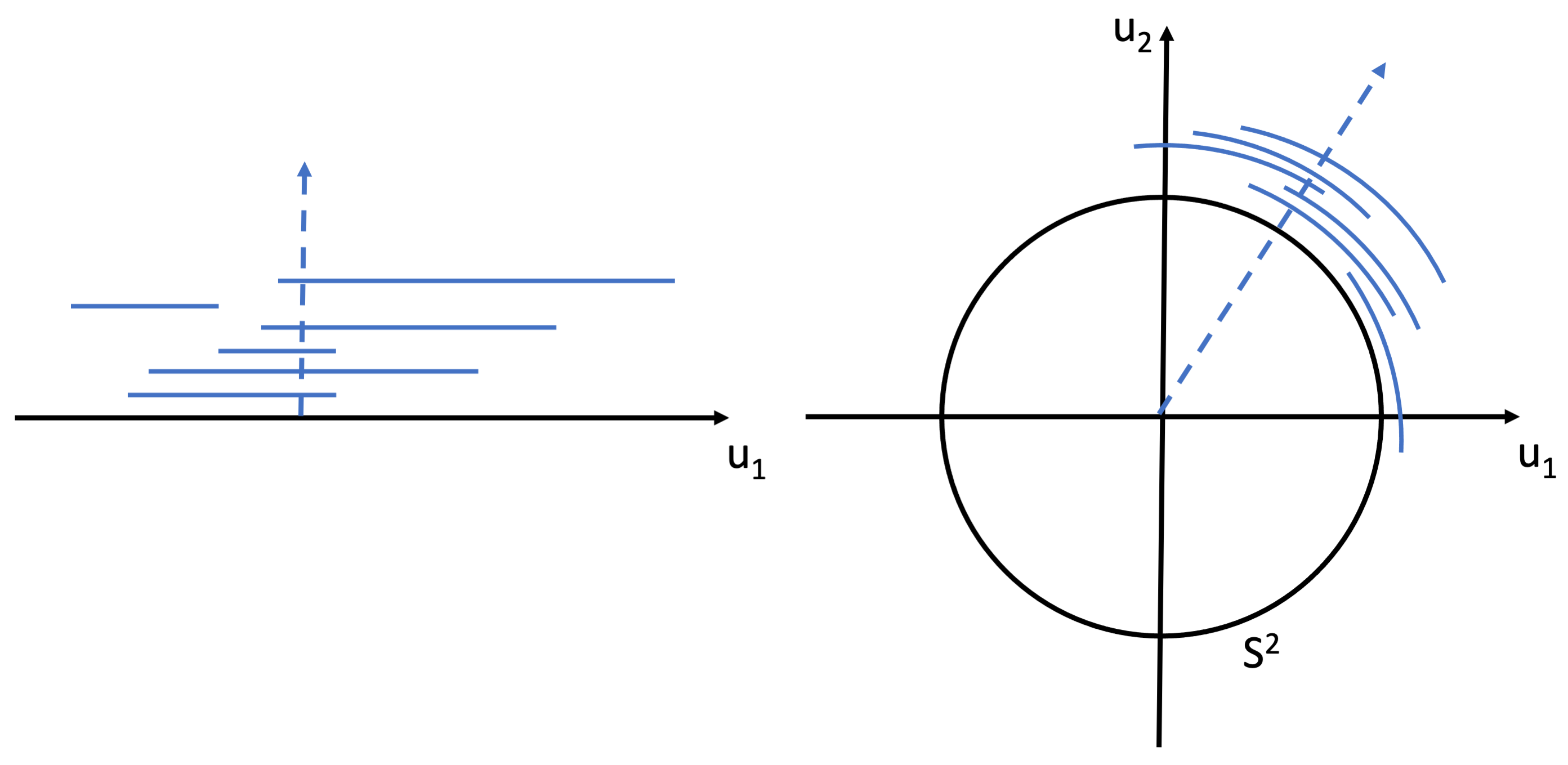
The challenge of the problem.
Each observation prescribes a region ,
The set captures all the possible values of that is consistent with the -th observation. The following lemma states that the set can be expressed by a group of linear constraints.
Lemma 1.
For each , there exists a matrix and a vector such that
In the deterministic setting of the revealed preference problem, all the ’s are identical and the learning problem is thus reduced to finding one feasible in the set of . But in a stochastic setting, it may happen that the set of is empty. Figure 1 provides a conceptual visualization of this challenge of “empty intersection”. Each blue solid segment denotes one such and the blue dashed line represents a value of that appears most frequently in these ’s. We remark that the figure is just for illustrative purpose as the problem may not be well-defined in the 1-dimensional case.
From an estimation viewpoint, the goal is to estimate the distribution of without the knowledge of the realized samples ’s, but merely with the knowledge of to which belongs. The sample efficiency of the estimation procedure is naturally contingent on the dispersion of which is essentially determined by the generation of For example, if all the ’s coincide with each other, then one can hardly learn much about the underlying In this paper, we aim to pinpoint conditions for such that the learning of is possible. Also, an alternative way to measure the estimation accuracy is to evaluate the predictive performance of the estimated model on new observations generated from and such performance bounds generally bear less dependency on the distribution of We also provide theoretical guarantees in this sense.
3 Gaussian Setting
In this section, we consider a setting where the distribution follows the von Mises-Fisher distribution parameterized by with the density function
Here the vector represents the mean direction and the parameter controls the concentration of the distribution. The deterministic setting of the revealed preference problem can be viewed as the case when and then the distribution degenerates to a point-mass distribution on the unit sphere. Denote the true parameters of the distribution by Then the likelihood of the dataset under a parameter is
We remark that the maximum likelihood approach cannot be applied here for two reasons. First, the integration of over the region is not closed-form. The first point is not only pertaining to the Gaussian parameterization of . The scale-invariant property of the utility vector restricts the distribution to a unit sphere or a simplex, and consequently, the likelihood function inevitably involves the non-closed-form integration. This issue can be partially resolved by using the Monte Carlo method to approximate the integration, and a good thing is that the same integrand is shared across all the observations. Second, the likelihood function is not analytical in . Thus this prevents the usage of gradient-based algorithms to solve the problem and also makes it difficult to derive theoretical guarantees for the maximum likelihood estimator.
We propose a Bayesian perspective for the problem: instead of identifying the parameter that maximizes the likelihood function, we directly draw samples from the posterior distribution. We will see shortly that the approach can be justified through a concentration property of the posterior distribution. Suppose we have a prior distribution and then we can define the posterior distribution by
With slight abuse of notation, we use (or ) to refer to both the density function and the probability measure of the posterior (or prior) distribution. We make the following assumption on the prior distribution.
Assumption 2.
We assume the concentration parameter where are two known positive constants. The prior distribution is a uniform distribution on .
Theorem 1.
Let
where is the Wasserstein distance between two distributions supported on equipped with Euclidean metric. Then, under Assumptions 1-2,
for any . Specifically, the following inequality holds
where the expectation is taken with respect to the random distribution (essentially, with respect to the dataset )
Theorem 1 justifies the approach of posterior sampling. We first remark that the Bayesian sampling approach is just proposed to estimate the parameters, but all the theoretical results are stated in frequentist language. The proof of Theorem 1 follows the standard analysis of the convergence of the posterior distribution (Ghosal et al. 2000; Chae et al. 2021). While similar results should also hold for other underlying distribution of , the von Mises-Fisher distribution provides much analytical convenience in deriving the bound. Each , together with the distribution of , defines a distribution over the space of . As we use observations ’s to identify the true , the set defines a set of indistinguishable ’s based on the Wasserstein distance between distributions of . The set shrinks as The posterior sampling approach samples from the distribution and Theorem 1 states that the samples will be concentrated in set with high probability. The posterior distribution is dependent on the dataset so it is a random distribution itself and the results in Theorem 1 are stated in either convergence in probability or expectation. As a side note, the Wasserstein distance in the theorem is not critical and it can be replaced with other distances such as the total variation distance and the Hellinger distance.
Intuitively, Theorem 1 says that for some such that the likelihood distribution differs from to a certain extent, the posterior is unlikely to generate such In other words, the posterior distribution identifies the true up to some “equivalence” in the likelihood distribution space. The following corollary formalizes this intuition that if there is an equivalence between the likelihood distribution space and the underlying parameter space, then the posterior distribution is capable of identifying the true parameter.
Corollary 1.
Suppose
for all . Then the posterior distribution will converge to the point-mass distribution on almost surely as . Moreover, suppose there exists a constant satisfying
| (1) |
for all .
The corollary states that when there is some equivalence between the likelihood distribution space and the parameter space as (1), the true parameter is identifiable. The first part of the corollary states a consistency result that as long as all the are distinguishable from through the likelihood function, then the posterior sampling will eventually identify the true The second part relates to the convergence rate with an equivalence parameter .
In Assumption 1, we assume the constraint input is generated from some distribution We note that Theorem 1 and Corollary 1 hold without any additional assumption on , but the space topology of the likelihood distribution is highly dependent on Specifically, a different distribution of determines the separateness of the parameter space through affecting the value of in (1) or even its existence. The value of a specific distribution of can be examined through simulation. So if the learner has some flexibility in choosing the distribution of , the optimal choice would be the one that corresponds to a larger value of If the constraint input is not randomly generated but can be actively chosen as the query-based preference learning problem, the results in Theorem 1 and Corollary 1 still hold by conditioning on all the ’s. Unlike the deterministic case where the utility vector is fixed for all the observations, the stochastic nature of the problem setup here makes it generally very complicated to fully extract the benefit of designing ’s by the learner. We leave it as a future open question.
Corollary 2.
Suppose is a discrete distribution with a finite support. Let be a new sample from , i.e., independent from the dataset , and let be a sample from the posterior distribution Denote and as the optimal solutions of LP and LP, respectively. Then, under Assumptions 1-2, the following inequality holds with probability no less than ,
where the expectation is taken with respect to both the posterior distribution and
Corollary 2 provides an upper bound on the predictive performance of the posterior distribution. Specifically, we want to predict the optimal solution of a linear program specified by (proportionally to ) and a new sample of the constraint , and the prediction is based on a posterior sample. We know from Theorem 1 that the posterior distribution concentrates on those ’s that are indistinguishable from the true in terms of the likelihood. Speaking of the predictive performance, we only concern the distribution of the optimal solution (equivalently, the likelihood), but do not require the identification of exact true so Corollary 2 does not require the condition (1) to hold. Intuitively, the prediction of the optimal solution on a new observation can be viewed as a condition distribution of the optimal solution given . While the definition of in Theorem 1 concerns the joint distribution of the optimal solution and , the finite-support condition on in Corollary 2 transforms the result on the joint distribution to the conditional distribution.
4 -Corruption Case
In this section, we consider a setting where the utility vector is specified by
| (2) |
where is a fixed vector, , and is an arbitrary distribution that corrupts the inference of . The deterministic setting of the revealed preference problem in literature can be viewed as the case of , and the Gaussian setting in the previous section can be viewed as the case of and being the von-Mises Fisher distribution. In this setting, we do not aim to learn the distribution of , but rather our goal is to identify the vector using the dataset
A natural idea to estimate is by solving the following optimization problem:
where the indicator function if and otherwise. The rationale for the optimization problem is that for the -th observation, a vector is consistent with the observation, i.e., is the optimal solution of LP, if and only if . Thus the optimization problem finds a vector that is consistent with the maximal number of observations. The objective function is discontinuous in , so we propose the simulated annealing algorithm – Algorithm 2 to solve for its optimal solution.
We first build some connection between the optimization problem OPTδ and that of the deterministic setting with . Let be the optimal solution of LP and define
Then the deterministic setting of the revealed preference problem solves
By the setup of the problem, is an optimizer of and the optimal objective value is The following proposition establishes that the optimization problem OPTδ is a contaminated version of and the effect that the contamination has on the objective function can be bounded using .
Proposition 1.
Under Assumption 1, the following inequality holds
When the constraints ’s are generated from some distribution it can happen that there exist some vectors that are indistinguishable from based on the observations as in the previous Gaussian case. So, we do not hope for an exact recovery of , but alternatively, we aim to derive a generalization bound for our estimator . Specifically, we define and analyze the accuracy
where is our estimator of , is a new sample from the distribution , is a new sample following the law of (2), and is the optimal solution of LP. In other words, the quantity captures the probability that is consistent with a new (unseen) observation, and we know that for the true parameter, , which serves as a performance benchmark.
The challenge for deriving a bound on arises from the discontinuity of the objective function OPTδ. The existing methods for deriving generalization bound largely rely on the continuity and the Lipschitzness of the loss function. To make it worse, from Lemma 1, we know that is specified by and the ’s are of different dimensions for different ’s. To overcome these challenges, we devise the following -margin objective function. Specifically, we first define a parameterized version of by
where is a positive constant and is an all-one vector. It is obvious that Accordingly, we define the -margin optimization problem by
Proposition 2.
Proposition 2 relates the generalization accuracy of any arbitrary with the corresponding objective value of the -margin optimization problem. As increases, the objective function will decrease, so the right-hand-side becomes tighter. Importantly, the accuracy is defined by the original indicator function (or equivalently, ), while the objective value is defined by the -margin indicator function (or equivalently, ). The implication is that when we optimize the -margin objective, we can still obtain a bound on the original accuracy Acc for sufficiently large .
Theorem 2.
Suppose is a continuous distribution and it has a density function upper bounded by . Then, under Assumption 1, the following inequality holds
where is one optimal solution of with .
Theorem 2 states a generalization bound on the accuracy of for continuous distributions of From Proposition 2, a larger leads to a smaller gap between the accuracy and the -margin objective function. Meanwhile, a smaller leads to a smaller gap between the optimal objective value OPT and . In the extreme case of , Theorem 2 optimizes the value of to trade off these two aspects. We note that the continuous distribution and the upper bound on the density function make it possible to bound the gap of the second aspect. Finally, we remark that the design of -margin loss function is inspired from the max-margin classifier, but the analysis is entirely different. For the max-margin classifier, the introduction of the margin aims to make the underlying loss function 1-Lipschitz so that a generalization bound using Rademacher complexity can be derived. But for here, our -margin objective function is still a discontinuous one.
5 Computational Aspects and Discussions
In the previous section, we developed theoretical results for both Gaussian and -corruption settings. Now we discuss computational aspects with respect to the sampling of the posterior and the optimization of OPT As mentioned earlier, the posterior sampling removes the complication of optimizing over in the maximum likelihood estimation, but still inevitably needs to deal with the sampling and numeric approximation of the likelihood function. Algorithm 1 describes a standard Metropolis–Hastings algorithm to sample from the posterior distribution In the numerical experiments, we choose the proposal distribution to be a Gaussian random perturbation, i.e., where follows a Gaussian distribution and the projection ensures that stays on the sphere For the acceptance ratio, as the posterior distribution is not in closed form, a Monte Carlo subroutine is needed to estimate the ratio.
| (3) |
Algorithm 2 presents a simulated annealing algorithm to solve the optimization problem OPT in Section 4. It takes a similar MCMC routine as Algorithm 1 and we use the same Gaussian random perturbation for the proposal distribution . As the temperature parameter decreases, the sampling distribution in Algorithm 2 will gradually be more concentrated on the optimal solution set of OPT. Algorithm 2 can be implemented more efficiently than Algorithm 1 in that the likelihood ratio calculation in (3) is analytical.
Table 1 reports some numerical results for the two algorithms. For both the Gaussian and -corruption settings, we consider three distributions of : (i) a uniform distribution where Unif and Unif; (ii) a discrete distribution where and Unif; (iii) a fixed- distribution where and Unif. For the Gaussian case, the true parameters are uniformly generated from , and the accuracy is calculated by where and are defined in Corollary 2. For the Gaussian case, is uniformly generated from and is set to be , and the accuracy is calculated by AccAcc where Acc is defined in Section 4. The numbers in Table 1 are reported based on an average of 20 simulation trials, and we run both Algorithm 1 and Algorithm 2 for iterations.
We make the following observations from the numerical experiments. First, we remark that the theoretical results in the previous sections provide strong guarantees on the convergence property of the posterior distribution. So the deterioration of the algorithm performance for the case when is solely caused by the inaccuracy of the approximate sampling in either Algorithm 1 or Algorithm 2. Such inaccuracy can definitely be mitigated to some extent by a more efficient algorithm implementation such as parallel computing. However, we argue that the performance deterioration as grows may point to a curse of dimensionality that is intrinsic to this estimation problem. Essentially, we aim to estimate a high-dimensional distribution only through partial information, i.e., the sets ’s. On the positive end, the algorithms work well for so if the learner has the power of choosing , s/he can break up the high-dimensional estimation problem into a number of low-dimensional estimation problems by focusing on a handful of dimensions each time. Moreover, we provide a visualization of the condition (1) in Figure 2 for calculated based on simulation. The visualization supports the existence of and thus the identifiability of the true parameters when the posterior sampling can be accurately fulfilled. 0
| (i) | 99.9% | 99.9% | 98.8% | 59.9% | |
| Gaussian | (ii) | 99.9% | 99.3% | 96.9% | 56.9% |
| (iii) | 99.9% | 94.8% | 92.6% | 68.5% | |
| (i) | 99.9% | 96.7% | 96.0% | 55.7% | |
| -corru. | (ii) | 99.6% | 97.9% | 97.6% | 63.1% |
| (iii) | 99.9% | 98.7% | 87.1% | 58.7% |

We conclude our discussion with the following remarks.
Query-based model with learner-chosen : In this paper, we have focused on the case where the constraints ’s are stochastically generated. When the concentration parameter is known for the Gaussian case, there is an efficient way of learning through choosing ’s (See the Appendix). In addition, the numerical experiments above also inspire a method that dismantles the high-dimensional estimation problem into a number of low-dimensional problems. Another interesting and important question is whether there exist designs of ’s such that the posterior sampling can be more efficiently carried out.
Multiple constraints and nonlinear utility: The results in this paper are presented under the setting of a linear objective and a single constraint. We emphasize that the results can be easily generalized to the case of multiple constraints and parameterized nonlinear utility. Thus our result can be viewed as a preliminary effort to address the problem of stochastic inverse optimization. Our conjecture is that when the set corresponds to a multiple-constraint problem, it may feature more structure and thus facilitate the learning of the utility distribution.
Choice modeling: The stochastic utility model in our paper also draws an interesting connection with the literature on choice modeling, which is a pillar for the pricing and assortment problems in revenue management (Talluri et al. 2004; Gallego et al. 2019). For most of the existing choice models, the learning problem can be viewed as a special case of our study by letting and . The results in our paper complement to this line of literature in developing a model where customers can make multiple purchases.
References
- Afriat (1967) Afriat, Sydney N. 1967. The construction of utility functions from expenditure data. International economic review 8(1) 67–77.
- Ahuja and Orlin (2001) Ahuja, Ravindra K, James B Orlin. 2001. Inverse optimization. Operations Research 49(5) 771–783.
- Amin et al. (2015) Amin, Kareem, Rachel Cummings, Lili Dworkin, Michael Kearns, Aaron Roth. 2015. Online learning and profit maximization from revealed preferences. Proceedings of the AAAI Conference on Artificial Intelligence, vol. 29.
- Aswani et al. (2018) Aswani, Anil, Zuo-Jun Shen, Auyon Siddiq. 2018. Inverse optimization with noisy data. Operations Research 66(3) 870–892.
- Balcan et al. (2014) Balcan, Maria-Florina, Amit Daniely, Ruta Mehta, Ruth Urner, Vijay V Vazirani. 2014. Learning economic parameters from revealed preferences. International Conference on Web and Internet Economics. Springer, 338–353.
- Baricz (2010) Baricz, Árpád. 2010. Bounds for modified bessel functions of the first and second kinds. Proceedings of the Edinburgh Mathematical Society 53(3) 575–599.
- Bärmann et al. (2018) Bärmann, Andreas, Alexander Martin, Sebastian Pokutta, Oskar Schneider. 2018. An online-learning approach to inverse optimization. arXiv preprint arXiv:1810.12997 .
- Beigman and Vohra (2006) Beigman, Eyal, Rakesh Vohra. 2006. Learning from revealed preference. Proceedings of the 7th ACM Conference on Electronic Commerce. 36–42.
- Bertsimas et al. (2012) Bertsimas, Dimitris, Vishal Gupta, Ioannis Ch Paschalidis. 2012. Inverse optimization: A new perspective on the black-litterman model. Operations research 60(6) 1389–1403.
- Besbes et al. (2021) Besbes, Omar, Yuri Fonseca, Ilan Lobel. 2021. Contextual inverse optimization: Offline and online learning. Available at SSRN 3863366 .
- Birge et al. (2017) Birge, John R, Ali Hortaçsu, J Michael Pavlin. 2017. Inverse optimization for the recovery of market structure from market outcomes: An application to the miso electricity market. Operations Research 65(4) 837–855.
- Boucheron et al. (2013) Boucheron, Stéphane, Gábor Lugosi, Pascal Massart. 2013. Concentration inequalities: A nonasymptotic theory of independence. Oxford university press.
- Burton and Toint (1992) Burton, Didier, Ph L Toint. 1992. On an instance of the inverse shortest paths problem. Mathematical programming 53(1) 45–61.
- Chae et al. (2021) Chae, Minwoo, Pierpaolo De Blasi, Stephen G Walker. 2021. Posterior asymptotics in wasserstein metrics on the real line. Electronic Journal of Statistics 15(2) 3635–3677.
- Chen and Kılınç-Karzan (2020) Chen, Violet Xinying, Fatma Kılınç-Karzan. 2020. Online convex optimization perspective for learning from dynamically revealed preferences. arXiv preprint arXiv:2008.10460 .
- Dong et al. (2018a) Dong, Chaosheng, Yiran Chen, Bo Zeng. 2018a. Generalized inverse optimization through online learning. Advances in Neural Information Processing Systems 31.
- Dong and Zeng (2020) Dong, Chaosheng, Bo Zeng. 2020. Expert learning through generalized inverse multiobjective optimization: Models, insights, and algorithms. International Conference on Machine Learning. PMLR, 2648–2657.
- Dong et al. (2018b) Dong, Jinshuo, Aaron Roth, Zachary Schutzman, Bo Waggoner, Zhiwei Steven Wu. 2018b. Strategic classification from revealed preferences. Proceedings of the 2018 ACM Conference on Economics and Computation. 55–70.
- Gallego et al. (2019) Gallego, Guillermo, Huseyin Topaloglu, et al. 2019. Revenue management and pricing analytics, vol. 209. Springer.
- Ghosal et al. (2000) Ghosal, Subhashis, Jayanta K Ghosh, Aad W Van Der Vaart. 2000. Convergence rates of posterior distributions. Annals of Statistics 500–531.
- Gibbs and Su (2002) Gibbs, Alison L, Francis Edward Su. 2002. On choosing and bounding probability metrics. International statistical review 70(3) 419–435.
- Gray (2011) Gray, Robert M. 2011. Entropy and information theory. Springer Science & Business Media.
- Keshavarz et al. (2011) Keshavarz, Arezou, Yang Wang, Stephen Boyd. 2011. Imputing a convex objective function. 2011 IEEE international symposium on intelligent control. IEEE, 613–619.
- Liese and Vajda (2006) Liese, Friedrich, Igor Vajda. 2006. On divergences and informations in statistics and information theory. IEEE Transactions on Information Theory 52(10) 4394–4412.
- McAllester (2003) McAllester, David A. 2003. Pac-bayesian stochastic model selection. Machine Learning 51(1) 5–21.
- Mohajerin Esfahani et al. (2018) Mohajerin Esfahani, Peyman, Soroosh Shafieezadeh-Abadeh, Grani A Hanasusanto, Daniel Kuhn. 2018. Data-driven inverse optimization with imperfect information. Mathematical Programming 167(1) 191–234.
- Romanazzi (2014) Romanazzi, Mario. 2014. Discriminant analysis with high dimensional von mises-fisher distributions. 8th Annual International Conference on Statistics. Athens Institute for Education and Research, 1–16.
- Samuelson (1948) Samuelson, Paul A. 1948. Consumption theory in terms of revealed preference. Economica 15(60) 243–253.
- Talluri et al. (2004) Talluri, Kalyan T, Garrett Van Ryzin, Garrett Van Ryzin. 2004. The theory and practice of revenue management, vol. 1. Springer.
- Van der Vaart (2000) Van der Vaart, Aad W. 2000. Asymptotic statistics, vol. 3. Cambridge university press.
- Varian (2006) Varian, Hal R. 2006. Revealed preference. Samuelsonian economics and the twenty-first century 99–115.
- Zadimoghaddam and Roth (2012) Zadimoghaddam, Morteza, Aaron Roth. 2012. Efficiently learning from revealed preference. International Workshop on Internet and Network Economics. Springer, 114–127.
- Zhang and Liu (1996) Zhang, Jianzhong, Zhenhong Liu. 1996. Calculating some inverse linear programming problems. Journal of Computational and Applied Mathematics 72(2) 261–273.
Appendix A Auxiliary Lemmas
We present some preliminary lemmas in this section. Most of them are basic inequalities in Information Theory, so they are only for auxiliary purposes in our proofs of the main theorems and the corollaries.
Lemma 2 (Pinsker’s inequality).
For any two distributions and ,
where denotes the total variation distance between two distributions, and denotes the KL-divergence between distributions.
Proof.
We refer to Lemma 6.2 of the book Gray 2011. ∎
Lemma 3 (Data processing inequality).
Let be a set of random variables indexed by parameter in some space . Consider two random variables taking values in . The following inequality holds
where denotes the KL-divergence between two distributions. Here is also called a Markov kernel, a transition probability distribution, or a statistical kernel.
Proof.
We refer to Theorem 14 of the article Liese and Vajda 2006. ∎
Lemma 4 (Packing number).
Let denote the ball in centered at original point with radius . Then, the -packing number of is bounded by
In other words, there exist at most disjoint balls in .
Proof.
Assume that there are disjoint -balls. Then, the total volume of those balls cannot be larger than the volume of a ball, i.e.,
which implies
∎
Lemma 5 (Hoeffding’s inequality).
Let be independent random variables such that takes its values in almost surely for all Then for every
Proof.
We refer to Chapter 2 of the book (Boucheron et al. 2013). ∎
Lemma 6 (Doob’s consistency theorem).
Suppose that whenever . Then, for every prior probability measure on the parameter space, the sequence of posterior measures converges to the point mass distribution of the true parameter in distribution for almost every .
Proof.
We refer to 10.10 of the book Van der Vaart 2000. ∎
Lemma 7.
Let be a set of functions whose domain is the support of the distribution of . For any probability distribution on , the following inequality holds for all and all distributions on simultaneously
with probability no less than . Here the inner expectation on the left-hand-side is taken with respect to
Proof.
We refer to Theorem 1 of the article McAllester 2003. ∎
The following lemma provides a useful bound for the modified Bessel function of the first kind. This function is closely related to the density of the von Mises–Fisher distribution. Typically, the modified Bessel function of the first kind is denoted by with the parameter . In this paper, to distinguish between the indicator function and this modified Bessel function, we denote the modified Bessel function by .
Lemma 8.
For all and ,
where denotes the modified Bessel function of the first kind.
Proof.
We refer to Chapter 2 of the article Baricz 2010. ∎
Appendix B Proof of Section 3
In this section, we provide the proofs of Section 3 and analyze the convergence of the posterior distribution. As we mentioned earlier, the Wasserstein distance in Theorems 1 is not essential, and all other equivalent metrics or weaker metrics are also valid, such as the total variation distance, the Hellinger distance and the Prokhorov metric (See Gibbs and Su 2002 for more about the relationships between different probability metrics). In this section, we show that Theorem 1 holds with respect to the total variation distance, and then explain how to obtain the result for the Wasserstein distance from there. The main idea is inspired by Ghosal et al. 2000. In this section, we first state and show several key lemmas and then prove the main theorem.
B.1 Key Lemmas for the Proof of Theorem 1
Recall is the data set, and is the likelihood distribution under the parameter . In the following, we denote the parameter space by , denote the total variation distance between and by , where are two parameters, and denote the -packing number of a parameter subset with a metric by For example, if the underlying metric is the total variation metric, the corresponding -packing number is denoted by
Lemma 9 (Lemma 7.1 in (Ghosal et al. 2000)).
Suppose the -packing number of the parameter space with the total variation distance is bounded by some positive constant , i.e.,
Then, for , there exist a function , which maps a dataset with samples to , such that
| (4) | ||||
| (5) |
where the expectation is taken with respect to the underlying dataset under a distribution specified by the corresponding parameter.
Proof.
We refer to Lemma 7.1 in Ghosal et al. 2000. ∎
Intuitively, the lemma states that if the packing number is bounded, we can find a function such that its expectation is close to when taken under a distribution with the true parameter, and it is close to 1 otherwise. In statistics, the function naturally serves as a test. In the proof of Theorem 1, we will see that this test function plays an important role in bounding the numerator of the posterior distribution.
To apply this lemma for the proof of Theorem 1, we first bound the packing number to meet the lemma’s condition. Here denotes the KL divergence between two distributions.
Lemma 10.
For any two parameters and in ,
| (6) |
Furthermore, we have
Proof.
The first inequality comes directly from Pinsker’s inequality (Lemma 2). From Lemma 3, we have
where
which is independent of the choice of , and denotes the modified Bessel functions of the first kind. Here, the first line comes from Lemma 3. The second line comes from the definition of the KL-divergence and the density function of the von Mises–Fisher distribution, and the third line comes from the definition of . The fourth line comes from Lemma 8 that
and the last line comes from Cauchy inequality that
Therefore, the -ball centered at some with the L2-norm is a subset of the -ball centered at with the total variation metric, i.e.,
Thus, the -packing number of with the total variance metric is bounded by the -packing number of with the L2-norm, that is,
Finally, by Lemma 4, for all , we have
∎
We will use the above two lemmas to bound the numerator of the posterior distribution. First, we derive a lower bound of the denominator of the posterior distribution. And then we will combine those two parts to establish the statement of the posterior distribution.
Lemma 11.
For any , the following inequality holds with probability no less than ,
| (7) |
Proof.
Let
By inequality (6) in Lemma 10, we have that contains the -ball centered at with the -norm and, therefore,
| (8) |
Next, we show that with probability no less than ,
| (9) |
Since the range of the density function of is between for all , we have that
for all . Then, by Hoeffding’s inequality (Lemma 5), we have, with probability no more than ,
| (10) |
where the first line comes directly from Hoeffding’s inequality, the second line comes from Fubini’s theorem, and the last line comes from the definition of . Then, by Jensen’s inequality,
| (11) | ||||
B.2 Proof of Theorem 1
In this part, we combine three lemmas in the previous section and show Theorem 1.
Proof.
Let
By Lemma 11, we have, with probability no less than , the inequality
| (12) |
holds for all satisfying . In (B.2), we will use this inequality to establish a lower bound for the denominator of the posterior distribution.
By Lemma 10, we have for all
which gives an upper bound of the packing number and thus verifies the condition of Lemma 9. Then, by Lemma 9, for all , there exists a function mapping the data set to , which satisfies
| (13) | ||||
| (14) |
Let
We then have
| (15) | ||||
where the first line is obtained by Fubini’s theorem, the second line is obtained directly by computing the inner integral, and the last line comes from the definition of and inequality (14). Denote the low probability event corresponding to inequality (12) as . By combining (12) and (B.2), we have
| (16) |
where the first equality comes from the definition of the posterior distribution, and the second line is obtained by plugging in (12) and (B.2).
Finally, we have
| (17) | ||||
where the first line comes from the fact that the posterior probability is bounded by 1, the second line comes from (13) and (B.2), and the last line comes from the definition of . The inequality above also indicates that converges to 1 in norm, which implies the convergence in probability. In fact, with a little modification for the bound in Lemma 11, we can get rid of the parameter in the definition of , and the expectation can be bounded by from below.
To obtained a similar result for the Wasserstein distance, we only need to establish the relationship between and . Notice that is independent of and the maximum distance between two points in is no larger than . We have
Thus, the result of (B.2) also holds for the Wasserstein distance metric if we have an additional factor in the definition of and , which is exactly in Theorem 1. ∎
B.3 Proof of Corollary 1
Proof.
The convergence of the posterior distribution to the point mass distribution can be directly obtained by Doob’s consistency theorem (Lemma 6). Here, we only show the second part, i.e., the upper bound of the posterior expectation . Without loss of generality, we assume that .
From the proof of Theorem 1, we have that, there exists a high probability event satisfying
such that
Then, by Markov’s inequality, we have for all
| (18) | ||||
where the first line comes from a decomposition of the event, the second line comes from Markov’s inequality, and the last line comes from the fact that and .
Next, from the condition (1),
Consequently, for any , we have
| (19) |
Combining (B.3) and (19), we have with probability no less than
Here, the first inequality is obtained by the fact the the maximum distance between two different parameters are bounded by , and the second inequality is obtained by (19). ∎
B.4 Proof of Corollary 2
Proof.
Recall the definition of
In a similar way as (B.3), we obtain
Then we utilize the total variation distance to bound the difference between optimal solutions. From the integral representation of the total variation distance, we have, for any ,
| (20) |
On the right hand side, the ratio is the probability that the optimal solutions (corresponding to and ) coincide for a fixed pair of . Thus, the integration calculates the probability that the the optimal solution corresponding to is different from the optimal solution corresponding to . Let be a random parameter drawn from the posterior distribution. Denote as the optimal solution corresponding to given , and as the optimal solution corresponding to given . We have
| (21) |
Thus, with probability no less than , we have
where the first line comes from the fact that the maximum distance between any two solutions is bounded by , the second line comes from (21), and the last line comes from the definition of .
We remark that the statement is also true for general distributions by replacing the probability ratio in (20) with the Radon–Nikodym derivative.
∎
Appendix C Proof of Section 4
In this section, we prove the results in Section 4.
C.1 Proof of Lemma 1
Proof.
For an observation of , let
From the LP’s optimality conditions, we know that if and only if the following three inequalities hold:
| (22) | ||||
| (23) | ||||
| (24) |
All the three inequalities can be expressed by linear constraints, so we finish the proof. ∎
C.2 Proof of Proposition 1
Proof.
The proof is a direct application of Hoeffding’s inequality. Denote as the indicator function of . By Hoeffding’s inequality, we have
Then, it is sufficient to show that
To see this, we have
where the first inequality is obtained by the fact that if , the second line comes from Jensen’s inequality for the absolute value function, and the last two lines come directly from the property of indicator functions. ∎
C.3 Proof of Proposition 2
Proof.
In this part, we will show a stronger statement that, for all ,
where the uniform bound holds for all in the unit ball (instead of unit sphere).
We will utilize Lemma 7 to prove the above inequality. For any in the unit ball, let and be two normal distributions over the estimated parameter space, where is the -dimensional identity matrix and is a constant to be determined. We remark that our choice of and will not affect the distribution of , which depends on , , , and . Thus, by Lemma 7, the following inequality holds with probability no less than ,
| (25) |
where denotes the complement of a set We note that on the left-hand-side, the inner expectation is taken with respect to the indicator function, and the outer expectation is taken with respect to
Then we have
| (26) | ||||
Here, the first line is obtained by calculating of the KL-divergence between two Gaussian distributions, and the second line is a further simplification of the second line.
Now we analyze the left-hand-side and show that
| (27) |
To see this, for a fixed , if , at least one inequalities from (22) to (24) is violated. If (22) does not hold for while , there exists at least one such that
The corresponding probability is no less than , which is bounded by . Following the same analysis for (23) and (24), we have with probability no more than ,
which gives the left part of (27). The right part follows the same analysis.
Thus, let . From (27) and (26), we have, with probability no less than , the following inequalities hold simultaneously for all in the unit ball,
| (28) | ||||
where the first inequality is obtained by plugging (27) into both sides of (26), the second line is obtained by plugging the value of into the inequality, and the last line is obtained by the convexity of the square root function. Finally, with probability no less than
where the first line comes from the fact that holds for any point and set , and the second line comes from (C.3) with replacing by . ∎
C.4 Proof of Theorem 2
In this part, we assume that the optimal solution satisfies
This assumption is natural in that if purchasing the -th item brings no positive utility, the customer will not purchase the item.
The proof is divided into two parts. In the first part, we show that, if is sufficiently small, with high probability, the margin indicator is almost same as . In the second part, we combine the first part and Proposition 2 to draw the conclusion. Intuitively, the smaller is, the smaller the difference between and we will have, and the worse the bound in Proposition 2 will be. Then the second part trades off between these two aspects and chooses the best . The formal proof is stated as below.
Proof.
Let
where is an optimal solution of . Now, let us show that holds with probability no less than . By definition of and the assumption that for all , we have and
for any , and . Moreover, for any such that , we have
which happens with probability no more than . Since there are at most index pairs, with probability no less than , we have
| (29) |
Then, similar to the proof of Lemma 1 with Hoeffding’s inequality, we have
where the randomness in the above inequalities comes only from . Here, the inequality comes from the analysis of (29) and Hoeffding’s inequality.
Next, we combine the above analysis and Proposition 2. Let be the optimal solution of the problem . Then, we have, for any , with probability no more than ,
| (30) | ||||
where the first inequality is obtained by Proposition 2, the second line is obtained by the optimality of , the third line is obtained by a similar statement as Proposition 1, the fourth line comes from (29), and the last line is obtained by the fact that for all . Finally, plug and into (C.4). If is sufficient large such that , we have, with probability no less than ,
We remark that we can further reduce the dependency of by setting . ∎
Appendix D Gaussian setting with Known Concentration Parameter
In this section, we revisit the Gaussian setting and discuss two methods to learn the mean vector when the concentration parameter is known. Specifically, we consider the following two cases : (i) We can design the constraint pair for all , (ii) We can only design for all while we know a lower bound such that for all . The basic idea is to estimate for every and to use the idea of “moment matching” to identify .
Constraint Design for the First Case
For the first case, we set and for all . Then, at each time , we have if and only if . We can then estimate by the sample average mean
Next, we estimate based on .
For any , let be an angle in satisfying . By Lemma 1 from Romanazzi 2014, we have
| (31) |
which depends only on . Thus, with slight abuse of notation, we denote as the probability in (31). Moreover, if , we can have that the above function is strictly increasing. Then, by Lemma 1 from Romanazzi 2014 with the induction method, we can show that the above function is strictly increasing with respect to for every fixed and . For any fixed and , we first numerically compute (31). Then, a natural estimate of is
Then, is our estimation of . We can further normalize in case that .
We remark that this method can be hardly generalized to the case that is unknown. The reason is that we do not have a similar strictly increasing structure, and that the bijection between the probability (31) and the parameter might not exist.
Constraint Design for the Second Case
Now we discuss how to design if we cannot control . One difficulty that prevents us applying the same method as in the previous section is that we might have while due to an insufficient budget. However, if we know a lower bound of , we can still estimate by dismantling the high-dimensional estimation problem into a number of low-dimensional problems.
Denote the lower bound as . We set the first entries in be and others be , where denotes the ceiling function. In this case, we have
In this way, we can estimate for following the previous case. To estimate the probability for other , we can divide the problem into parts and estimate the probabilities separately.