Modified Bivariate Weibull Distribution Allowing Instantaneous and Early Failures

In reliability analysis and life data analysis, Weibull distribution is used mostly because of its versatility. In literature, extension and generalization of the Weibull distribution are given in Pham and Lai, 2007, Murthy et al., 2004, El-Gohary and El-Morshedy, 2015. In life testing experiments, mainly in electronic parts and clinical trials, many items fail instantaneously or fail early due to faulty construction or inferior quality or due to no response of the treatments. We record the observed lifetime is close to zero. To model life data containing such nearly instantaneous failure, traditional parametric distributions, for example, Weibull distribution, Pareto distribution, exponential distribution, gamma distribution, log-normal distribution, etc., are not accurate in practice as such failures in experiment usually discard the assumption of a uni-modal distribution. These situations can be modeled by modifying the traditionally used parametric distributions. Muralidharan and Lathika, 2006, modified the two parameters Weibull distribution by mixing two-parameter Weibull distribution and a singular distribution at zero. Lai et al., 2007 modified the two parameters Weibull distribution by considering the mixture of the uniform distribution and two parameters Weibull distribution. Muralidharan and Khabia, 2011, model this instantaneous or early failures data by considering the mixture of the uniform distribution and the Pareto distribution. To estimate the model parameters, maximum likelihood estimation is used mainly. Muralidharan et al., 2011, estimated the model parameters using Bayesian approach. Cheng and Sheu, 2016 proposed M-estimation method and derived the closed form of the shape parameter estimation. Using simulation study they showed that, M-estimation performs better than the MLE for samples with early failure. To model data with inliers (instantaneous or early failure), non-standard mixture of distributions, with degeneracy occurring at zero and one, and a probability distribution for positive observation is used mainly. Muralidharan and Bavagosai, 2018 estimates the parameters of such model on the basis of type-II censored sample from a Weibull distribution with discrete mass at zero and one. To model instantaneous failure data from clinical trials and longitudinal, Withana Gamage et al., 2020 proposed two methods to estimate the parameters and used expectation-maximization(EM) algorithm. Muralidharan and Bavagosai, 2021 provided a method for testing hypothesis to find statistical significance of the single and multiple inliers in samples.

Many data in real life are bivariate in nature and correlated, which contains huge observation near a particular point $(x_{0},y_{0})$ and other responses follow some continuous distribution; we define this as early failure data. If that particular point is origin, i.e. $(x_{0},y_{0})=(0,0)$, we call it as nearly instantaneous failure data. Bivariate Weibull distribution using FGM copula and there some properties are proposed in literature Almetwally et al., 2020, Peres et al., 2018. However, we did not find any modeling technique to fit such correlated bivariate data with instantaneous or nearly instantaneous failure observations adequately in the literature. Here, we propose a modified bivariate Weibull distribution allowing early failure by considering the mixture of the bivariate uniform distribution and bivariate Weibull distribution. The bivariate Weibull distribution is obtained using a copula and two parameters Weibull distribution as marginal distribution. The forms of the survival function and hazard function are obtained by using a generalization of the Farlie-Gumbel-Morgenstern (GFGM) copula given by Lai and Xie, 2000. Furthermore, we consider the model to deal with the presence of nearly instantaneous failure $[(x_{0},y_{0})=(0,0)]$ in the responses and obtained the form of the hazard function and survival function using the GFGM copula. To illustrate the proposed model, in the simulation study, we consider the Gaussian copula [Nelsen, 2007] to construct the modified bivariate Weibull distribution. To estimate the parameters, we use the method of maximum likelihood estimation (MLE) and density-based spatial clustering of applications with noise (DBSCAN) clustering given by Ester et al., 1996.

The remainder of the article is organized as follows. We provide a brief review of copula functions and Sklar’s theorem for constructing multivariate distribution functions using the known marginals in Section 2. In Section 3, we construct a bivariate Weibull distribution function using a copula having two parameters Weibull distributions as marginals. We propose a modified Weibull distribution for early and instantaneous failure bivariate observations along with their hazard functions and the survival functions in Sections 4 and 5. Estimation of unknown parameters using the MLE combined with DBSCAN clustering process is described in Section 6. In Section 7, we provide an algorithm to simulate data from modified bivariate Weibull distribution. Numerical examples with simulated data are given in Section 8.1, and the proposed method is applied to real data in 8.2. The concluding remarks are given in Section 9.

In this section, copula function and how it can be used to form multivariate joint probability mass function from its marginals are discussed. For more information about copula we refer Nelsen, 2007, Joe, 2014 and Song and Song, 2007.

In copula theory, Sklar’s theorem [Sklar, 1959] is a fundamental result and we can use it to form a joint distribution from its marginal distributions.

A copula is a multivariate probability distribution with uniform marginal distributions on the interval $[0,1]$. Copulas are popular because of their ability to model dependence among $Y_{1},Y_{2}\cdots,Y_{d}$. Here is some examples of copula

The Gaussian copula density (Arbenz, 2013) is given by

where $\textbf{U}=\left[\Phi^{-1}(y_{1}),\Phi^{-1}(y_{2}),\ldots,\Phi^{-1}(y_{d})\right]^{T}$, $(y_{1},y_{2},\ldots,y_{d})\in[0,1]^{d}$, $\Phi$ is the univariate standard normal distribution and $R$ is the correlation matrix of the standard multivariate Gaussian distribution and $I_{d}$ be the $d\times d$ identity matrix.

Therefore, the density function of the GFGM copula is given by

where $(x,y)\in[0,1]^{2}$, $a\geq 1,\ b\geq 1$ and $-1\leq\rho\leq 1$.

Let us recall the definition of two parameters Wibull distribution. We denote $W\sim Wb(\alpha,\beta)$, if a random variable $W$ follows Weibull distribtuion with parameters $(\alpha,\beta)$ with the CDF given by

and the PDF given by

Let $X\sim Wb(\alpha_{1},\beta_{1})$ and $Y\sim Wb(\alpha_{2},\beta_{2})$ follow two parameter Weibull distribution with parameters $(\alpha_{1},\beta_{1})$ and $(\alpha_{2},\beta_{2})$ respectively with $\alpha_{1},\beta_{1},\alpha_{2},\beta_{2}>0$. Therefore the joint CDF of the bivariate Weibull distribution using a 2-dimensional copula $C$ and Sklar’s theorem is given by

where $x>0$, $y>0$ and $F_{X},F_{Y}$ are the CDF of the random variables X and Y respectively.

The joint probability density function (PDF) of the bivariate Weibull distribution is given by

where $x>0$, $y>0$ and $f_{X}(x),\ f_{Y}(y)$ are the PDF of the random variables X and Y respectively.

Now, we consider the GFGM copula (2.6) to find the form of the joint CDF and joint PDF of the bivariate Weibull distribution. For simplicity of the expressions, we define notation for some commonly used term as

Therefore, the joint CDF of the bivariate Weibull distribution using the GFGM copula (2.6) is given by

where $x>0$, $y>0$, $\alpha_{1}>0$, $\beta_{1}>0$, $\alpha_{2}>0$, $\beta_{2}>0$, $a\geq 1$, $b\geq 1$, $-1\leq\rho\leq 1$ and $F_{X}(x)$, $F_{Y}(y)$ are the CDF of $X$ and $Y$ respectively.
Therefore, the joint PDF $f_{XY}$ of the bivariate Weibull distribution is given by

where $x>0$, $y>0$, $\alpha_{1}>0$, $\beta_{1}>0$, $\alpha_{2}>0$, $\beta_{2}>0$, $a\geq 1$, $b\geq 1$, $-1\leq\rho\leq 1$.

By taking restrictions on $a$ and $b$, we can get a simplified form of the bivariate Weibull distribution functions.

• 1.

  If we choose $a=1,b=1$, the form of the joint CDF is

  $$\begin{split}F_{XY}(x,y)=&F_{X}(x)F_{Y}(y)[1+\rho(1-F_{X}(x))(1-F_{Y}(y))]\\ =&\left[1-\exp\left(-A\right)\right]\left[1-\exp\left(-B\right)\right]\left[1+\rho\exp\left[-\left(C\right)\right]\right]\end{split}$$

  (3.8)

  where $x>0$, $y>0$, $\alpha_{1}>0$, $\beta_{1}>0$, $\alpha_{2}>0$, $\beta_{2}>0$, $0\leq\rho\leq 1$.
  Therefore the corresponding joint PDF of the bivariate Weibull distribution is

  $$\begin{split}f_{XY}(x,y)=&\dfrac{\alpha_{1}\alpha_{2}}{\beta_{1}\beta_{2}}A^{1-1/\alpha_{1}}B^{1-1/\alpha_{2}}\exp(-C)\left[1+\rho\left(2\exp\left(-A\right)-1\right)\left(2\exp\left(-B\right)-1\right)\right]\end{split}$$

  (3.9)

  where $x>0$, $y>0$, $\alpha_{1}>0$, $\beta_{1}>0$, $\alpha_{2}>0$, $\beta_{2}>0$, $-1\leq\rho\leq 1$.

Here we find the distribution function of the modified Weibull distribution and the form of the survival function and hazard function.

Consider $(x_{0},y_{0})=(0,0)$ as a special case of the modified model (4.1), which is called as nearly instantaneous failure model. In this case the survival functions and hazard function for the bivariate uniform distribution are given by

and

The survival functions and hazard function for the modified bivariate Weibull model with nearly instantaneous failure occurring uniformly over the rectangle $[0,d]\times[0,d]$ is given by

and

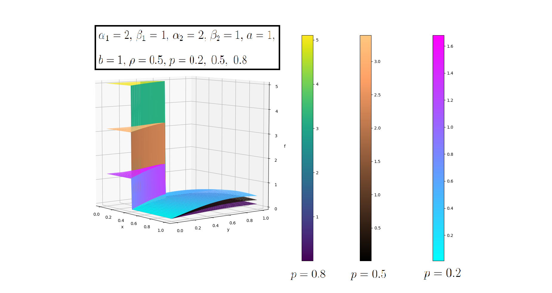
Graphical plots are important to identify whether the models useful for specific data sets for which empirical plots are available. For the instantaneous failure case, the graph of the MBW density function, survival function and hazard rate function are given for specific parameter values in the following way.

• 1.

  Density function: The plot of the density functions for the parameter values $\alpha_{1}=2$, $\beta_{1}=1$, $\alpha_{2}=2$, $\beta_{2}=1$, $a=1$, $b=1$, $\rho=0.5$, $d=0.4$ and $p=0.2,\ 0.5,\ 0.8$ are given in Figure 1.

• 2.

  Survival function: Corresponding to the density functions given in Figure 1, the plot of the survival functions are given in Figure 2.

• 3.

  Hazard function: The plot of the hazard function are given in the Figures 3, 4, 5 and 6 for different parameters. We can observe that the graph is similar to the Weibull hazard function outside the rectangle $[0,d]\times[0,d]$. Inside the rectangle, the behavior of the hazard function has more than one direction where it takes increasing, decreasing, and bathtub shape.

We estimate the unknown parameters of the proposed model using the MLE combined with the DBSCAN algorithm as follows. The joint PDF of the modified bivariate Weibull distribution allowing early and instantaneous failures is given by

where $f_{XY}$ is the joint PDF of bivariate Weibull distribution given in (3.4). The unknown parameters of the model are given by $\Theta=\{\alpha_{1},\beta_{1},\alpha_{2},\beta_{2},\bm{\rho},d,p\}$ with $\bm{\rho}$ representing copula parameters. To estimate the parameters $\Theta$, we combine the MLE technique and the DBSCAN clustering method in the following way.
Let $(x_{i},y_{i}),\ i=1,2,\cdots,n$ be the $n$ sample points from the population with PDF given by (6.1). Then, the likelihood function is

and the corresponding log-likelihood function is

We usually maximize the log-likelihood function to find the estimates of unknown parameters of the models by differentiating the likelihood or log-likelihood function with respect to the parameters and solving the equations simultaneously. However, we do not get a definite solution for d by the said approach due to the particular nature of the likelihood function concerning the corresponding variable. Now, we see that the log-likelihood function decreases as the value of d increases. So, the maximum log-likelihood function value occurred at the minimum possible value of d. Now, the contribution of d in the likelihood function is non-zero when d satisfies the following inequalities: $0<x_{i}<d$ and $0<y_{i}<d$ where $x_{i}$ and $y_{i}$ are independently generated from uniform distribution in [0,d]. So, we classify the data using the DBSCAN clustering method given by Ester et al., 1996. The DBSCAN parameters are estimated using the methodologies provided in Schubert et al., 2017 and Rahmah and Sitanggang, 2016. Then two clusters are formed; one is C1, generated from the bivariate uniform distribution, and another C2 from bivariate Weibull distribution. Now, we find the maximum likelihood estimate of d given by,

Then, we use the usual approach of finding the MLEs of other parameters by maximizing the log-likelihood function using the estimated value $\hat{d}$. In the numerical examples given in Section 8, we use R-packages “optim" and “dbscan" for estimating the model parameters using the proposed method.

In this section, we discuss an algorithm for simulating data (x,y) from the MBW distribution given in (4.1). The steps are as follows:

1. 1.

   Generates a value z from binomial distribution B(1,p).

2. 2.

   If $z=1$, then Generate x and y independently from the uniform distribution $U(0,d)$.

3. 3.

   If $z=0$, then generates (x,y) from the bivariate Weibull distribution given in (3.4), in the following way;

   1. (a)

      Generate $u$ and $t$ independently from uniform $(0,1)$.

   2. (b)

      Let $v=C^{-1}_{u}(t)$, where $C^{-1}_{u}$ is the quasi-inverse of $C_{u}$. Here, $C_{u}$ is defined as, $C_{u}:=P(V\leq v|U=u)=\dfrac{\partial C(u,v)}{\partial u}$, where C is a bivariate copula.
      In the case of the GFGM copula, we can find $v$ by solving the following equation using the Newton Raphson iteration method.

      $$v+\rho bu^{b-1}v^{b}(1-u)^{a}(1-v)^{a}-\rho au^{b}v^{b}(1-u)^{a-1}(1-v)^{a}-t=0$$

   3. (c)

      Set $x=F_{1}^{-1}(u)$ and $y=F_{2}^{-1}(v)$, where $F_{1}$ and $F_{2}$ are the CDF of univariate Weibull distribution with parameters $(\alpha_{1},\beta_{1})$ and $(\alpha_{2},\beta_{2})$ respectively.

To simulate n-data points using this algorithm we repeat these three steps n times.

Here, we provide numerical examples using simulated data to illustrate and test the proposed methodologies and apply them to real data.

References

- Almetwally et al., (2020) Almetwally, E. M., Muhammed, H. Z., and El-Sherpieny, E.-S. A. (2020). Bivariate weibull distribution: properties and different methods of estimation. Annals of Data Science, 7(1):163–193.
- Arbenz, (2013) Arbenz, P. (2013). Bayesian copulae distributions, with application to operational risk management—some comments. Methodology and computing in applied probability, 15(1):105–108.
- Cheng and Sheu, (2016) Cheng, Y.-F. and Sheu, S.-H. (2016). Robust estimation for weibull distribution in partially accelerated life tests with early failures. Quality and Reliability Engineering International, 32(7):2207–2216.
- El-Gohary and El-Morshedy, (2015) El-Gohary, A. and El-Morshedy, M. (2015). Bivariate exponentiated modified weibull extension. arXiv preprint arXiv:1501.03528.
- Ester et al., (1996) Ester, M., Kriegel, H.-P., Sander, J., Xu, X., et al. (1996). A density-based algorithm for discovering clusters in large spatial databases with noise. In kdd, volume 96, pages 226–231.
- Joe, (2014) Joe, H. (2014). Dependence modeling with copulas. CRC press, Florida.
- Lai et al., (2007) Lai, C., Khoo, M. B., Muralidharan, K., and Xie, M. (2007). Weibull model allowing nearly instantaneous failures. Journal of Applied Mathematics and Decision Sciences, 2007.
- Lai and Xie, (2000) Lai, C. and Xie, M. (2000). A new family of positive quadrant dependent bivariate distributions. Statistics & probability letters, 46(4):359–364.
- Muralidharan and Bavagosai, (2018) Muralidharan, K. and Bavagosai, P. (2018). A new weibull model with inliers at zero and one based on type-ii censored samples. Journal of the Indian Society for Probability and Statistics, 19(1):121–151.
- Muralidharan and Bavagosai, (2021) Muralidharan, K. and Bavagosai, P. (2021). Some inferences on tests for inliers. International Journal of Statistics and Reliability Engineering, 8(2):243–263.
- Muralidharan and Khabia, (2011) Muralidharan, K. and Khabia, A. (2011). A modified pareto distribution. J Indian Stat Assoc, 49:73–90.
- Muralidharan and Lathika, (2006) Muralidharan, K. and Lathika, P. (2006). Analysis of instantaneous and early failures in weibull distribution. Metrika, 64(3):305–316.
- Muralidharan et al., (2011) Muralidharan, K., Parikh, R., and Lai, C. (2011). A bayesian analysis on weibull model allowing nearly instantaneous failures. Reliability: Theory & Applications, 6(4 (23)):140–148.
- Murthy et al., (2004) Murthy, D. P., Xie, M., and Jiang, R. (2004). Weibull models, volume 505. John Wiley & Sons.
- Nelsen, (2007) Nelsen, R. B. (2007). An introduction to copulas. Springer Science & Business Media.
- Peres et al., (2018) Peres, M. V. d. O., Achcar, J. A., and Martinez, E. Z. (2018). Bivariate modified weibull distribution derived from farlie-gumbel-morgenstern copula: a simulation study. Electronic Journal of Applied Statistical Analysis, 11(2):463–488.
- Pham and Lai, (2007) Pham, H. and Lai, C.-D. (2007). On recent generalizations of the weibull distribution. IEEE transactions on reliability, 56(3):454–458.
- Rahmah and Sitanggang, (2016) Rahmah, N. and Sitanggang, I. S. (2016). Determination of optimal epsilon (eps) value on dbscan algorithm to clustering data on peatland hotspots in sumatra. In IOP conference series: earth and environmental science, volume 31, page 012012. IOP Publishing.
- Schubert et al., (2017) Schubert, E., Sander, J., Ester, M., Kriegel, H. P., and Xu, X. (2017). Dbscan revisited, revisited: why and how you should (still) use dbscan. ACM Transactions on Database Systems (TODS), 42(3):1–21.
- Sklar, (1959) Sklar, M. (1959). Fonctions de repartition an dimensions et leurs marges. Publ. inst. statist. univ. Paris, 8:229–231.
- Song and Song, (2007) Song, X.-K. and Song, P. X.-K. (2007). Correlated data analysis: modeling, analytics, and applications. Springer Science & Business Media, New York.
- Vannman, (1991) Vannman, K. (1991). Comparing samples from nonstandard mixtures of distributions with applications to quality comparison of wood. research report 1991:2. submitted to division of quality technology, Lulea University, Lulea, Sweden.
- Withana Gamage et al., (2020) Withana Gamage, P. W., Chaudari, M., McMahan, C. S., Kim, E. H., and Kosorok, M. R. (2020). An extended proportional hazards model for interval-censored data subject to instantaneous failures. Lifetime data analysis, 26(1):158–182.