Engineering chiral topological superconductivity in twisted Ising superconductors

Transition metal dichalcogenides (TMD) are van der Waals (vdW) materials and can be prepared as 2D atomic crystals. They have attracted considerable interest and have demonstrated rich electronic phenomena ranging from charge-density wave order, superconducitivity, exciton formation to the optical control of the valley degrees of freedom [1, 2, 3, 4, 5]. Strikingly, when prepared in few-layer forms, the so-called Ising superconductors gated-2H-MoS₂, 2H-NbSe₂, 2H-TaS₂, 2H-NbS₂ and 2H-TaSe₂ have anomalously large in-plane upper critical field, several times beyond the Pauli limit [6, 7, 8, 9, 10, 11]. The physical reason for this behavior can be attributed to strong Ising spin-orbit coupling in these materials, which pins the electrons’ spin along the $z$-direction and is much less susceptible to an in-plane magnetic field.

Due to their 2D nature, TMD allow the fabrication of various vdW heterostructures with flexible tunability and interplay between electronic structures, superconductivity and magnetism. For instance, the ferromagntic proximity effect in monolayer TMD has been well characterized in heterostructures such as WSe₂/CrI₃ [12, 13, 14] via optical probes. More recently, ferromagnetic Josephson junction NbSe₂/Cr₂Ge₂Te₆/NbSe₂ have been fabricated and investigated, and unconventional Josephson phase is reported [15, 16].

On the other hand, a new paradigm in the engineering of quantum phases of matter has been recently developed based on moiré patterns [17, 18, 19] introduced by stacking 2D crystals with twisting angles. Motivated by the discovery of correlated insulators and superconductivity in twisted bilayer graphene, the idea of moiré engineering has been extended into other materials including TMD [20, 21, 22, 23].

Interestingly, recent theories pointed out that twisted bilayer cuprate (Bi2212) may realize chiral topological superconductivity with nonzero Chern numbers [24, 25, 26] — a novel state of matter that yet to be experimentally confirmed, which has triggered further experimental and theoretical investigations [27, 28]. The crucial mechanism of realizing nontrivial topology here is based on the nodal superconductivity, due to sign changes of the pairing order parameter around the Fermi surface. Intuitively, nodal superconductors are naturally located on the boundary between trivial and nontrivial band topology, and engineering topological phases via perturbations becomes possible.

In order to fabricate moiré structures, vdW 2D crystals are highly desirable. Practically, however, Bi2212 may be the only known nodal superconductor among vdW 2D crystals. This puts forward a serious constraint on the moiré-engineering of topological superconductivity. For example, the TMD superconductors are known to be nodeless and s-wave superconductors, despite theoretical discussions on the role played by magnetic fluctuations in the pairing mechanism [29]. It would be unfortunate if they cannot be included in the moiré-engineering of topological superconductivity, especially considering their fabricational flexibililty and tunability.

Motivated by these experimental and theoretical efforts, we ask the following question: is it possible to moiré-engineer topological superconductivity in TMD superconductors? The answer is positive. We find that twisted Ising superconductors like 2H-NbSe₂ and 2H-TaS₂ in the presence of an proximity-induced in-plane Zeeman field (beyond the Pauli limit) and out-of-plane supercurrent can host chiral topological superconductivity with Chern number 12 or 6. The topological phases are found to be robust and occupies physically realizable parameter regimes. Under proper experimental conditions the topological pairing gap is $>0.1$meV.

Not surprisingly, the mechanism underlying our proposal still involves pairing-gap-closing nodes, required by a trivial-to-topological phase transition. Here the pairing nodes are induced by the in-plane Zeeman field (beyond the Pauli limit) for Ising superconductors with Fermi pockets around the $\Gamma$-point in the momentum space. These Zeeman-field induced nodes were firstly pointed out theoretically by He et.al. [30], and experimental evidences for such nodal states in the presence of an external magnetic field have been reported [31, 32, 9, 33].

Unlike the proposal based on cuprates [24, 25], here the topological superconductivity in TMD twisted bilayers is limited to low temperatures $\lesssim 1$K. Nevertheless, it is worth mentioning a few advantages of the present proposal. First, different from strongly-correlated cuprates, the TMD Ising superconductivity has been fairly well-understood as conventional s-wave pairing without strong correlations. Namely the low energy physics of TMD are well under control in terms of theoretical modelling. Second, detecting the chiral majorana edge modes is the smoking-gun experiment to identify chiral topological superconductivity. In the present proposal, these edge modes are sharply located at the edge of the ferromagnetic buffer layer, and can be detected using either thermal transport or scanning tunnelling microscope (STM) (see FIG.1 for an illustration). In the proposal based on cuprates, these edge modes will hybridize with the nodal superconductivity due to the irregular shape of the atomically thin flakes, and could be challenging to locate in real space.

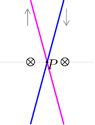
Unlike twisted bilayer graphene, twisted heterostructures of TMDs have two distinct configurations differ by a 180^∘ relative rotation, which were referred to as $\alpha$ and $\beta$ [34]. The $\alpha$-bilayer can be viewed as the building block for the bulk 2H-TMD structure, which restores the inversion symmetry. In this paper we instead focus on $\beta$-bilayer structure of Ising superconductors with Fermi pockets around the $\Gamma$-point (e.g. 2H-NbSe₂, 2H-TaS₂ but not gated 2H-MoS₂). In addition, a ferromagnetic insulating buffer layer with an in-plane magnetic moment is placed in the middle of the $\beta$-bilayer. At small twisting angles between the top and bottom TMD monolayers, we show that the system hosts chiral topological superconductivity when an out-of-plane supercurrent is present (see FIG.1 for an illustration).

Experimentally, most ferromagnetic vdW materials have an out-of-plane magnetic anisotropy. Only recently the monolayer CrCl₃ has been successfully isolated and confirmed to have an in-plane ferromagnetic order [12, 35]. On the other hand, theoretical first-principle calculations predicted that monolayer $\mathrm{Cr_{2}I_{3}Cl_{3}}$ [36], 2H-$\mathrm{VS_{2}}$ [37] and 2H-$\mathrm{VSe_{2}}$ [38, 39] should be insulators with in-plane ferromagnetic order. In addition, because of a weak magnetic anisotropy, the ferromagnetic moment in CrBr₃ can be re-oriented to an in-plane direction by a fairly small external magnetic field ($\sim 0.5$T)[40]. These vdW materials may serve as the ferromagnetic buffer layer in the present proposal.

Apart from the intrinsic electronic structures of the monolayer TMD, the proposed heterostructures are characterized by three parameters: the Zeeman exchange field $H_{\text{exch.}}$ induced by the magnetic proximity effect, the spin-independent interlayer hopping $t_{\perp}$, and the spin-dependent interlayer hopping $t_{s,\perp}$. These parameters depend on the choice of the buffer layer in the setup proposed in FIG.1(a). Moreover, one may consider more sophisticated multilayer setups as shown in FIG.1(b). By choosing different setups, in principle all the three parameters can be tuned individually.

In the simplest setup in FIG.1(a), $H_{\text{exch.}}$ and $t_{s,\perp}$ both are originated from the ferromagnetic buffer layer. In general there is no direct relation between them. However, in a mean-field treatment, the second-order perturbation theory gives $t_{s,\perp}=\mu_{B}H_{\text{exch.}}$ (see Appendix B). Although there is no available experimental data to quantify $H_{\text{exch.}}$ for the proposed heterostructures, similar heterostructures like WSe₂/CrI₃, MoSe₂/CrBr₃ with out-of-plane ferromagnetic layer have been well characterized experimentally and theoretically [41, 42, 43, 44, 45, 40], where a proximity-induced Zeeman splitting around $1\sim 2$meV is reported for electronic bands near the $K$ point. A similar value of splitting in the proposed heterostructures corresponds to $H_{\text{exch.}}=3\sim 6H_{p}$. Notice that monolayer NbSe₂ has been reported to sustain a in-plane upper critical field $6\sim 8H_{p}$ [31, 32, 9] (and about $9\sim 10H_{p}$ for TaS₂ [33, 46]).

We find that the topological phase is robust at least when a small twisting angle $\theta$ is comparable with $t_{\perp}/(\hbar v_{\text{Ising}}k_{F})$, where $k_{F}$ is the Fermi wavevector and the velocity $v_{\text{Ising}}$ is characterizing the Ising spin-orbit coupling near the $\Gamma$-$M$ direction (see Eq.(4)). It is convenient to introduce a dimensionless parameter to capture the ratio of the two quantities:

We consider proposed heterostructures involving either TaS₂ or NbSe₂. Their monolayer electronic structures are obtained using relaxed crystal structure based on first-principle calculations (see Appendix C for details). For each TMD material, two cases for the spin-dependent hopping $t_{s,\perp}$ are investigated, corresponding to:

We show the global phase diagram by tuning the spin-independent hopping $t_{\perp}$ and the Zeeman exchange field $H_{\text{exch.}}$ in FIG.2, based on numerical calculations. For presentation purpose, we have fixed $\xi^{\mathrm{TaS_{2}}}=0.9$ and $\xi^{\mathrm{NbSe_{2}}}=1.1$, and fixed the Josephson phase $\varphi=\pi/2$ corresponding the maximal supercurrent state. Topological superconducting phases are found to exist when $t_{\perp}\lesssim 9$meV for TaS₂ (and $t_{\perp}\lesssim 2.7$meV for NbSe₂). A Chern-number-12 phase is found to occupy a large portion of the parameter space, while a Chern-number-6 phase appears for case-(i) at small values of $t_{\perp}$. Under appropriate conditions, the gap in the topological phase can reach $0.1$meV.

These phase diagrams are also well-understood via analytical calculations. We have plotted the phase boundary (see Eq.(13)) between trivial and topological phases from our perturbative calculations in FIG.2, which is in good agreement with the numerical calculations.

Apart from the global phase diagrams, we also plot the phase diagrams with a few selected values of $t_{\perp}$. Fixing $H_{\text{exch.}}=4H_{p}$, we tune the twisting angle $\theta$ and the Josephson phase $\varphi$, and the results are shown in FIG.3. Consistent with the global phase diagram, the topological phase is realized when $t_{\perp}$ is not too large. Interestingly, for intermediate values of $t_{\perp}$, trivial to topological phase transitions are observed by tuning $\varphi$ alone while fixing the twisting angle $\theta$ in an appropriate regime. Such a Josephson-phase-driven topological transition in a single device can lead to unique features to unambiguously identify the topological phase in experiments. For instance, the gapless chiral majorana edge modes should appear only in the topological phase, after the phase transition occurs when $\varphi$ is tuned up.

In an in-plane Zeeman field regime $H_{\text{exch.}}>\sqrt{2}H_{p}$, it was pointed out that the pairing gap around the $\Gamma$-pockets will close and nodal superconductivity is formed [30], while the pairing gap around the $K$-pockets remain nodeless. These nodes on $\Gamma$-pockets turn out to be the origin of the topological superconductivity in the present proposal.

The minimal model for the bands forming the $\Gamma$-pockets (which has dominant $d_{z^{2}}$ orbital content of the transition metal) is as follows

Drastically different from the usual Rashba spin-orbit coupling, here the Ising spin-orbit coupling $\lambda^{\text{Ising}}_{\mathrm{SO}}(\bm{k})$ splits bands with fixed $S_{z}$-spin. In fact, due to the $z\rightarrow-z$ mirror symmetry of monolayer 2H-TMD, the Rashba spin-orbit coupling is forbidden. Time-reversal symmetry dictates that $\lambda^{\text{Ising}}_{\mathrm{SO}}(\bm{k})=-\lambda^{\text{Ising}}_{\mathrm{SO}}(-\bm{k})$, so $\lambda^{\text{Ising}}_{\mathrm{SO}}(\bm{k})$ necessarily has sign changes. Due to the mirror plane containing the $\Gamma$-$M$ axis, the six $\Gamma$-$M$ directions are exact where $\lambda^{\text{Ising}}_{\mathrm{SO}}(\bm{k})$ changes sign.

We therefore begin with a first-order $\bm{k\cdot p}$ model near the intersection point $P$ between the Fermi surface and one $\Gamma$-$M$ direction ($k_{x}$-direction, see Fig.4 for an illustration):

where $\lambda^{\text{Ising}}_{\mathrm{SO}}(\bm{k})$ vanishes along the $k_{x}$-direction, and $v_{\text{Ising}}\equiv\frac{\partial\lambda^{\text{Ising}}_{\mathrm{SO}}(\bm{k})}{\hbar\partial k_{y}}$. We list these parameters for NbSe₂ and TaS₂ in Table.1 based on first principle calculations (Fig. 5 plot the band structures, full list of quartic $\bm{k\cdot p}$ expansion parameters is given in Appendix C).

Monolayer: After introducing an spin-singlet pairing $\Delta$ ¹¹ 1 $\Gamma$-$M$ mirror symmetry protects that there is no singlet-triplet mixing at $P$-point., in the Nambu basis we obtain the BCS mean-field Hamiltonian:

where Pauli $\tau$-matrices label the particle-hole space, and an Zeeman field $H_{y}$ along the $y$-direction is introduced (the g-factor is assumed to be 2). Because the system has a spin-rotation symmetry around $S_{z}$-direction, the choice of the direction of the in-plane magnetic field is not important. Since there are three independent $\Gamma$-$M$-directions, related by $C_{3}$ rotations, the full electronic structure of NbSe₂ (TaS₂) has three copies of the effective theory in Eq.(5).

Eq.(5) can be solved straightforwardly. A pair of Dirac nodes are found to emerge when $\mu_{B}H_{y}>\Delta$, located at $\bm{k}^{\pm}=(\pm\frac{1}{\hbar v_{F}}\sqrt{(\mu_{B}H_{y})^{2}-\Delta^{2}},0)$ (see Fig.4) for a schematic illustration, consistent with earlier works [30, 29], whose low energy effective theories are:

where $\eta=\arcsin\frac{\Delta}{\mu_{B}H_{y}}$, $\delta\bm{k}$ is measured from the nodal points $\bm{k}^{\pm}$, and $\Sigma$ are Pauli matrices in the low energy space. These nodes are protected by a chiral symmetry $\sigma_{x}\tau_{y}$ in model Eq.(5) (corresponding to the combination of the physical time-reversal transformation $i\sigma_{y}K$, the particle-hole transformation $\tau_{x}K$ and a $S_{z}$-$\pi$ rotation $i\sigma_{z}\tau_{z}$) sending $h(\bm{k})\rightarrow-h(\bm{k})$.

Twisted bilayer: Next we consider a $\beta$-bilayer (separated by an insulator buffer layer) with a twisting angle $\theta$, which can be viewed as top/bottom monolayer twisted by angle $\pm\theta/2$ respectively. Introducing $k_{F}$ being the crystal momentum of point $P$, we obtain the following effective theory near $P$:

Here the Pauli matrices $\nu$ captures the top/bottom layer space. $\Delta>0$ and the pairing amplitude is $\Delta e^{\pm i\varphi/2}$ for the top/bottom layer respectively. The $t_{\perp}$ and $t_{s_{y},\perp}$ terms describes the spin-independent and spin-dependent interlayer hopping processes respectively. Based on the two-center approximation [19, 21], and the fact that point $P$ is far away from the Brillouin zone boundary, the interlayer hopping processes have a weak stacking-dependence, and are considered as constants in the present work [27, 28] (see Appendix E for a discussion on the two-center approximation).

The model Eq.(7) can be analytically solved in various perturbative regimes. To demonstrate the stability of the topological superconductivity, below we focus on one particular regime, in which $\sqrt{(\hbar v_{\text{Ising}}k_{F}\theta)^{2}+4t_{\perp}^{2}}\gg\Delta,\mu_{B}H_{y},t_{s_{y},\perp}$. The advantage of this regime is that it is always realizable in the proposed heterostructures by tuning the twisting angle $\theta$. In this regime, we find that the topological superconductivity with Chern number 4 (corresponding to Chern number 12 for the whole heterostructure) is always realized in model Eq.(7) by tuning $\varphi,\theta$ and $\mu_{B}H_{y}\gtrsim\Delta$.

To understand this behavior, we may firstly turn off the pairing $\Delta$ and $\mu_{B}H_{y},t_{s_{y},\perp}$ in model Eq.(7). There are four intersection points between the spin-up and spin-down Fermi surfaces, which we label as $C,D$ and $F,G$ and are located at the $k_{y}$ and $k_{x}$ axes respectively (see FIG. 6).

The low energy effective theory near each point resembles Eq.(4) with modified $v_{F}$ and $v_{\text{Ising}}$.

After $\Delta,\varphi$ are turned on but $\mu_{B}H_{y}=t_{s_{y},\perp}=0$, the pairing gap minima near $C,D,F,G$ are found to be the same $\Delta_{C,D,F,G}=\Delta\sqrt{\cos^{2}\frac{\varphi}{2}+\cos^{2}\xi\sin^{2}\frac{\varphi}{2}}$, where $\xi$ is defined in Eq.(1). Because the connection with the $\varphi=0$ limit, the superconducting phase so far must still be topologically trivial even though $\varphi\neq 0$ breaks the time-reversal symmetry.

When $\mu_{B}H_{y},t_{s_{y},\perp}\neq 0$ are tuned up, the behavior near the points $C,D$ versus $F,G$ are qualitatively different. The pairing gap minima near $F,G$ never go to zero as long as $\varphi\neq 0$. In particular, we find:

where

On the contrary, near points $C,D$ topological phase transition occurs with four Dirac nodes (two near each point) emerging when $H_{y}=H^{\text{topo.}}_{c}$, where the critical Zeeman field strength is

When $H_{y}>H^{\mathrm{topo.}}_{c}$ the four Dirac nodes acquire topological mass gap, transferring a Chern number of 4:

The details of the calculations are presented in Appendix D.

Note that different from $\Delta_{F,G}$, the topological gap $\Delta^{\text{topo.}}_{C,D}$ $\propto\Delta^{2}$. This is because $\Delta$-linear order gap remains zero in the present linear-order $\bm{k\cdot p}$ effective theory, and the second order perturbation plays the dominant role: the topological phase is always realized when $H_{y}>H^{\text{topo.}}_{c}$.

When a higher order $\bm{k\cdot p}$ expansion is considered, we do find that a non-topological $\Delta$-linear order gap near $C,D$ becomes nonzero (see Appendix D). When this gap is large the topological superconductivity will be destroyed. Based on perturbative calculations, the topological phase requires the following criterion to be satisfied (See Appendix D Eq.(59) for details):

Here $v_{2}$ is a velocity parameter (defined in Eq.(37)) in the quadratic-order $\bm{k\cdot p}$ expansion, $\hbar v^{\text{NbSe}_{2}}_{2}=0.94$ and $\hbar v^{\text{TaS}_{2}}_{2}=3.1$ eV$\cdot$Åbased on our electronic structure calculations (See Appendix C). Namely, $t_{\perp}$ cannot be too large. This criterion serves as the phase boundary between the trivial and topological phases, and is plotted in FIG.2 as the dashed black line.

The previous perturbative regime well captures the Chern-number-12 topological phase. Aiming at understanding the Chern-number-6 topological phase in the numerical phase diagrams, we have performed the analytical calculations in a different perturbative regime: $t_{\perp}\ll\Delta,\hbar v_{\text{Ising}}k_{F}\theta\ll\Delta$, and reproduced the Chern-number-6 topological phase (see Appendix D).

Before concluding, we would like to remark on a few experiment-related issues.

Chiral edge modes: When topological superconductivity is realized in the proposed heterostructure in Fig.1(a), the edge of the ferromagnetic buffer layer is the natural boundary between the topological superconductivity and trivial superconductivity. This is because outside the buffer layer region, due to the lack of Zeeman exchange field, gapped trivial superconductivity is realized in the TMD bilayer. Majorana chiral edge modes are then sharply located at this edge, leading to well-known quantized thermal Hall conductance $\frac{\kappa_{xy}}{T}=C\frac{\pi}{12}\frac{k_{B}^{2}}{\hbar}$, where $C$ is the Chern number. In addition, the edge modes can detected via scanning tunnelling microscopy as mid-gap states.

Mid-gap states located at the edge of a superconducting material has non-topological explanations, such as the Yu-Shiba-Rusinov bound states. However, in an appropriate regime, as shown in Fig.3, we note that a single device may realize trivial to topological phase transition while the Josephson phase $\varphi$ is tuned up. Such a $\varphi$-driven topological phase transition has unique experimental signatures since the majorana edge states are expected to exist only in the topological phase, which may be used to sharply identify the nature of the mid-gap states.

The effect of in-plane external magnetic field: When an in-plane magnetic field is applied to the proposed heterostructures, the Josephson phase $\varphi(x)=2\pi x/L$ becomes spatial dependent along the in-plane transverse direction, where $L=\frac{\Phi_{0}}{H_{\text{ext.}}d}$ and $d$ is the effective thickness of the junction. For instance, an external magnetic field $H_{ext.}\sim 0.5$T is needed to reorient the magnetic moment of CrBr₃ to an in-plane direction, corresponding to $L\sim 2\mu$m if $d\sim 20\text{\AA}$ is used. Due to the fact that the Chern number flips sign when $\varphi\rightarrow-\varphi$, the topological superconductivity is expect to form spatial stripes, or domains with width $L/2$, with alternating Chern numbers, e.g., $C=\pm 12$ in which case 24 chiral majorana states are expected to form at each domain-wall. In Appendix A we estimate the spatial spread $l_{\perp}$ of the domain-wall majorana states along the transverse direction of the domain-wall. Only when $l_{\perp}$ is much smaller than the stripe width $L/2$ are the domain-wall states well-defined. We find that for a generic magnetic field direction $l_{\perp}$ is comparable with $L/2$ for $H_{ext.}\sim 0.5$T. However, when $H_{ext.}$ is parallel to one $\Gamma-M$ direction, 8 among the 24 domain-wall majorana states have an $l_{\perp}$ that can be $5\sim 10$ times smaller than $L/2$. These domain wall chiral states may be observable in probes such as STM or thermal transport.

Charge-density-wave Order: It is known that Ising superconductivity in 2H-$\mathrm{NbSe_{2}}$ or 2H-$\mathrm{TaS_{2}}$ coexists with the charge-density-wave (CDW) order [48, 49, 50]. For the Fermi pockets around $\Gamma$, the Fermi surface folding due to CDW occurs near the $\Gamma$-$K$ direction, which would not qualitatively affect the low energy physics near the $\Gamma$-$M$ direction, which we have been focusing on in this paper.

Rashba Spin-orbit Coupling: As emphasized before, the $z\rightarrow-z$ mirror symmetry forbids the Rashba spin-orbit coupling in the monolayer TMD. A Rashba spin-orbit coupling breaks an important invariance of Eq.(7) related to the combination of particle-hole and time-reversal transformation $\mathsf{PH}\circ\mathsf{TR}=\sigma_{y}\tau_{x}$. $\mathsf{PH}\circ\mathsf{TR}$ always sends $h_{\text{BCS}}^{\text{bilayer}}(\bm{k},H_{y},\varphi)\mapsto-h_{\text{BCS}}^{\text{bilayer}}(\bm{k},-H_{y},-\varphi)$. In the absence of the Rashba spin-orbit coupling one may flip the sign of $H_{y}$ and $\varphi$ by a complex conjugation since all other terms in the Hamiltonian are real: $-h_{\text{BCS}}^{\text{bilayer}}(\bm{k},-H_{y},-\varphi)=-(h_{\text{BCS}}^{\text{bilayer}})^{*}(\bm{k},H_{y},\varphi)$. Namely there is an invariance protecting the Bogoliubov quasiparticle spectrum being $\pm E$ symmetric at any $\bm{k}$. Such an invariance is lost in the presence of a Rashba spin-orbit coupling, leading to Bogoliubov Fermi pockets [29].

In the proposed heterostructures, despite the lack of the $z\rightarrow-z$ mirror symmetry, the intrinsic Rashba coupling induced by the vdW interlayer interactions can be safely neglected since it is extremely weak (see in Appendix C). Although an extrinsic, substrate-induced Rashba coupling is possible, in this paper we do not consider this effect, since nevertheless this coupling could be tuned to zero via gating.

Interlayer Tunneling Strength: It is clear from the phase diagrams in FIG. 2 and criterion Eq.(13) that the interlayer tunneling $t_{\perp}$ cannot be too large in order to realize the topological superconductivity ($<10$meV). On the other hand, based on our DFT calculation (see Appendix C), due to the $d_{z^{2}}$ nature of Fermi pockets around $\Gamma$-point, a fairly large interlayer tunneling of the bilayer systems of $\mathrm{NbSe_{2}}$ or $\mathrm{TaS_{2}}$ without a buffer layer is found near the point-$P$ ($>50$meV) ²² 2 In literature https://www.nature.com/articles/s41467-018-03888-4, a smaller value of tunneling about 15meV for bilayer $\mathrm{NbSe_{2}}$ is reported. We ascribe such discrepancy to the choice of van der Waals pseudopotentials.. This actually motivates us to consider the insulating buffer layer in the proposed heterostructures. In Appendix C, as an estimate, we performed DFT calculations on a $\mathrm{TaS_{2}}/\mathrm{WS_{2}}/\mathrm{TaS_{2}}$ heterostructure, and $t_{\perp}\sim 5$meV is found – well within the regime where topological superconductivity is realized.

In summary, we theoretically propose twisted bilayer vdW Ising superconductors as a new flexible and tunable platform to realize chiral topological superconductivity with Chern numbers. In the simplest setup, an insulating buffer layer with an in-plane ferromagnetic moment is introduced between the TMD Ising superconductors such as $\mathrm{NbSe_{2}}$ or $\mathrm{TaS_{2}}$, providing Zeeman exchange field in the TMD layers via the magnetic proximity effect. We show that the out-of-plane supercurrent induces topological superconductivity over a large parameter regime, and the characteristic majorana chiral edge modes are localized on the edge of the ferromagnetic buffer layer. We hope that the present study may motivate further experimental and theoretical investigations on such vdW heterostructures.

Acknowledgement Y.R. and X.H. acknowledge the support from National Science Foundation under Grant No. DMR-1712128. We thank Di Xiao for helpful discussions. X.H. thanks the open discussion of distributive computation on JuliaDiscourse, and the HPC resources of Andromeda Cluster at Boston College.

References

- Lian et al. [2018] C.-S. Lian, C. Si, and W. Duan, Nano letters 18, 2924 (2018).
- He et al. [2020] M. He, P. Rivera, D. Van Tuan, N. P. Wilson, M. Yang, T. Taniguchi, K. Watanabe, J. Yan, D. G. Mandrus, H. Yu, et al., Nature communications 11, 1 (2020).
- Jones et al. [2013] A. M. Jones, H. Yu, N. J. Ghimire, S. Wu, G. Aivazian, J. S. Ross, B. Zhao, J. Yan, D. G. Mandrus, D. Xiao, et al., Nature nanotechnology 8, 634 (2013).
- Rivera et al. [2016] P. Rivera, K. L. Seyler, H. Yu, J. R. Schaibley, J. Yan, D. G. Mandrus, W. Yao, and X. Xu, Science 351, 688 (2016).
- Li et al. [2021a] W. Li, X. Lu, J. Wu, and A. Srivastava, Nature Nanotechnology 16, 148 (2021a).
- Costanzo et al. [2016] D. Costanzo, S. Jo, H. Berger, and A. F. Morpurgo, Nature nanotechnology 11, 339 (2016).
- Yan et al. [2019] R. Yan, G. Khalsa, B. T. Schaefer, A. Jarjour, S. Rouvimov, K. C. Nowack, H. G. Xing, and D. Jena, Applied Physics Express 12, 023008 (2019).
- Cho et al. [2021] C.-w. Cho, J. Lyu, C. Y. Ng, J. J. He, K. T. Lo, D. Chareev, T. A. Abdel-Baset, M. Abdel-Hafiez, and R. Lortz, Nature Communications 12, 3676 (2021), ISSN 2041-1723, URL https://doi.org/10.1038/s41467-021-23976-2.
- de la Barrera et al. [2018] S. C. de la Barrera, M. R. Sinko, D. P. Gopalan, N. Sivadas, K. L. Seyler, K. Watanabe, T. Taniguchi, A. W. Tsen, X. Xu, D. Xiao, et al., Nature Communications 9, 1427 (2018), ISSN 2041-1723, URL https://doi.org/10.1038/s41467-018-03888-4.
- Li et al. [2017] L. Li, X. Deng, Z. Wang, Y. Liu, M. Abeykoon, E. Dooryhee, A. Tomic, Y. Huang, J. B. Warren, E. S. Bozin, et al., npj Quantum Materials 2, 11 (2017), ISSN 2397-4648, URL https://doi.org/10.1038/s41535-017-0016-9.
- Lian et al. [2019] C.-S. Lian, C. Heil, X. Liu, C. Si, F. Giustino, and W. Duan, The Journal of Physical Chemistry Letters 10, 4076 (2019).
- Cai et al. [2019] X. Cai, T. Song, N. P. Wilson, G. Clark, M. He, X. Zhang, T. Taniguchi, K. Watanabe, W. Yao, D. Xiao, et al., Nano letters 19, 3993 (2019).
- Aivazian et al. [2015] G. Aivazian, Z. Gong, A. M. Jones, R.-L. Chu, J. Yan, D. G. Mandrus, C. Zhang, D. Cobden, W. Yao, and X. Xu, Nature Physics 11, 148 (2015).
- McGuire et al. [2017] M. A. McGuire, G. Clark, K. Santosh, W. M. Chance, G. E. Jellison Jr, V. R. Cooper, X. Xu, and B. C. Sales, Physical Review Materials 1, 014001 (2017).
- Ai et al. [2021] L. Ai, E. Zhang, J. Yang, X. Xie, Y. Yang, Z. Jia, Y. Zhang, S. Liu, Z. Li, P. Leng, et al., Nature communications 12, 1 (2021).
- Idzuchi et al. [2020] H. Idzuchi, F. Pientka, K.-F. Huang, K. Harada, Ö. Gül, Y. Shin, L. Nguyen, N. Jo, D. Shindo, R. Cava, et al., arXiv preprint arXiv:2012.14969 (2020).
- Cao et al. [2018a] Y. Cao, V. Fatemi, A. Demir, S. Fang, S. L. Tomarken, J. Y. Luo, J. D. Sanchez-Yamagishi, K. Watanabe, T. Taniguchi, E. Kaxiras, et al., Nature 556, 80 (2018a).
- Cao et al. [2018b] Y. Cao, V. Fatemi, S. Fang, K. Watanabe, T. Taniguchi, E. Kaxiras, and P. Jarillo-Herrero, Nature 556, 43 (2018b).
- Bistritzer and MacDonald [2011] R. Bistritzer and A. H. MacDonald, Proceedings of the National Academy of Sciences 108, 12233 (2011).
- Li et al. [2021b] H. Li, S. Li, M. H. Naik, J. Xie, X. Li, J. Wang, E. Regan, D. Wang, W. Zhao, S. Zhao, et al., Nature materials 20, 945 (2021b).
- Devakul et al. [2021] T. Devakul, V. Crépel, Y. Zhang, and L. Fu, Nature communications 12, 1 (2021).
- Angeli and MacDonald [2021] M. Angeli and A. H. MacDonald, Proceedings of the National Academy of Sciences 118 (2021).
- Wu et al. [2019] F. Wu, T. Lovorn, E. Tutuc, I. Martin, and A. MacDonald, Physical review letters 122, 086402 (2019).
- Can et al. [2021] O. Can, T. Tummuru, R. P. Day, I. Elfimov, A. Damascelli, and M. Franz, Nature Physics 17, 519 (2021).
- Song et al. [2021] X.-Y. Song, Y.-H. Zhang, and A. Vishwanath, arXiv preprint arXiv:2109.08142 (2021).
- Zhao et al. [2021] S. Zhao, N. Poccia, X. Cui, P. A. Volkov, H. Yoo, R. Engelke, Y. Ronen, R. Zhong, G. Gu, S. Plugge, et al., arXiv preprint arXiv:2108.13455 (2021).
- Volkov et al. [2020] P. A. Volkov, J. H. Wilson, and J. Pixley, arXiv preprint arXiv:2012.07860 (2020).
- Volkov et al. [2021] P. A. Volkov, S. Y. F. Zhao, N. Poccia, X. Cui, P. Kim, and J. Pixley, arXiv preprint arXiv:2108.13456 (2021).
- Shaffer et al. [2020] D. Shaffer, J. Kang, F. Burnell, and R. M. Fernandes, Physical Review B 101, 224503 (2020).
- He et al. [2018] W.-Y. He, B. T. Zhou, J. J. He, N. F. Yuan, T. Zhang, and K. T. Law, Communications Physics 1, 1 (2018).
- Xi et al. [2016] X. Xi, Z. Wang, W. Zhao, J.-H. Park, K. T. Law, H. Berger, L. Forró, J. Shan, and K. F. Mak, Nature Physics 12, 139 (2016).
- Xing et al. [2017] Y. Xing, K. Zhao, P. Shan, F. Zheng, Y. Zhang, H. Fu, Y. Liu, M. Tian, C. Xi, H. Liu, et al., Nano letters 17, 6802 (2017).
- Navarro-Moratalla et al. [2016] E. Navarro-Moratalla, J. O. Island, S. Manas-Valero, E. Pinilla-Cienfuegos, A. Castellanos-Gomez, J. Quereda, G. Rubio-Bollinger, L. Chirolli, J. A. Silva-Guillén, N. Agraït, et al., Nature communications 7, 1 (2016).
- Xian et al. [2019] L. Xian, D. M. Kennes, N. Tancogne-Dejean, M. Altarelli, and A. Rubio, Nano letters 19, 4934 (2019).
- Lu et al. [2020] X. Lu, R. Fei, L. Zhu, and L. Yang, Nature communications 11, 1 (2020).
- Zhang et al. [2020] F. Zhang, H. Zhang, W. Mi, and X. Wang, Physical Chemistry Chemical Physics 22, 8647 (2020).
- Fuh et al. [2016] H.-R. Fuh, C.-R. Chang, Y.-K. Wang, R. F. Evans, R. W. Chantrell, and H.-T. Jeng, Scientific reports 6, 1 (2016).
- Zhang et al. [2019] W. Zhang, L. Zhang, P. K. J. Wong, J. Yuan, G. Vinai, P. Torelli, G. van der Laan, Y. P. Feng, and A. T. Wee, ACS nano 13, 8997 (2019).
- Kezilebieke et al. [2020] S. Kezilebieke, M. N. Huda, P. Dreher, I. Manninen, Y. Zhou, J. Sainio, R. Mansell, M. M. Ugeda, S. van Dijken, H.-P. Komsa, et al., Communications Physics 3, 1 (2020).
- Aikebaier et al. [2022] F. Aikebaier, T. T. Heikkilä, and J. Lado, Physical Review B 105, 054506 (2022).
- Zhong et al. [2017] D. Zhong, K. L. Seyler, X. Linpeng, R. Cheng, N. Sivadas, B. Huang, E. Schmidgall, T. Taniguchi, K. Watanabe, M. A. McGuire, et al., Science advances 3, e1603113 (2017).
- Zhong et al. [2020] D. Zhong, K. L. Seyler, X. Linpeng, N. P. Wilson, T. Taniguchi, K. Watanabe, M. A. McGuire, K.-M. C. Fu, D. Xiao, W. Yao, et al., Nature Nanotechnology 15, 187 (2020).
- Seyler et al. [2018] K. L. Seyler, D. Zhong, B. Huang, X. Linpeng, N. P. Wilson, T. Taniguchi, K. Watanabe, W. Yao, D. Xiao, M. A. McGuire, et al., Nano letters 18, 3823 (2018).
- Zollner et al. [2019] K. Zollner, P. E. F. Junior, and J. Fabian, Physical Review B 100, 085128 (2019).
- Ciorciaro et al. [2020] L. Ciorciaro, M. Kroner, K. Watanabe, T. Taniguchi, and A. Imamoglu, Physical Review Letters 124, 197401 (2020).
- Pan et al. [2017] J. Pan, C. Guo, C. Song, X. Lai, H. Li, W. Zhao, H. Zhang, G. Mu, K. Bu, T. Lin, et al., Journal of the American Chemical Society 139, 4623 (2017).
- [47] Note1, - mirror symmetry protects that there is no singlet-triplet mixing at -point.
- Ugeda et al. [2016] M. M. Ugeda, A. J. Bradley, Y. Zhang, S. Onishi, Y. Chen, W. Ruan, C. Ojeda-Aristizabal, H. Ryu, M. T. Edmonds, H.-Z. Tsai, et al., Nature Physics 12, 92 (2016).
- Xi et al. [2015] X. Xi, L. Zhao, Z. Wang, H. Berger, L. Forró, J. Shan, and K. F. Mak, Nature nanotechnology 10, 765 (2015).
- Nakata et al. [2018] Y. Nakata, K. Sugawara, S. Ichinokura, Y. Okada, T. Hitosugi, T. Koretsune, K. Ueno, S. Hasegawa, T. Takahashi, and T. Sato, npj 2D Materials and Applications 2, 1 (2018).
- [51] Note2, in literature https://www.nature.com/articles/s41467-018-03888-4, a smaller value of tunneling about 15meV for bilayer is reported. We ascribe such discrepancy to the choice of van der Waals pseudopotentials.
- Yang et al. [2018] Y. Yang, S. Fang, V. Fatemi, J. Ruhman, E. Navarro-Moratalla, K. Watanabe, T. Taniguchi, E. Kaxiras, and P. Jarillo-Herrero, Physical Review B 98, 035203 (2018).
- [53] Note3, for few-layer , the relation is also reported to be in https://www.nature.com/articles/s41563-018-0061-1. Since such coefficient is material- and stacking-dependent, we will still take the value of BCS approximation as a demonstration.
- Giannozzi et al. [2009] P. Giannozzi, S. Baroni, N. Bonini, M. Calandra, R. Car, C. Cavazzoni, D. Ceresoli, G. L. Chiarotti, M. Cococcioni, I. Dabo, et al., Journal of physics: Condensed matter 21, 395502 (2009).
- Giannozzi et al. [2017] P. Giannozzi, O. Andreussi, T. Brumme, O. Bunau, M. B. Nardelli, M. Calandra, R. Car, C. Cavazzoni, D. Ceresoli, M. Cococcioni, et al., Journal of physics: Condensed matter 29, 465901 (2017).
- Pizzi et al. [2020] G. Pizzi, V. Vitale, R. Arita, S. Blügel, F. Freimuth, G. Géranton, M. Gibertini, D. Gresch, C. Johnson, T. Koretsune, et al., Journal of Physics: Condensed Matter 32, 165902 (2020).
- Tkatchenko and Scheffler [2009] A. Tkatchenko and M. Scheffler, Physical review letters 102, 073005 (2009).
- Berland et al. [2019] K. Berland, D. Chakraborty, and T. Thonhauser, Physical Review B 99, 195418 (2019).
- Lee et al. [2010] K. Lee, É. D. Murray, L. Kong, B. I. Lundqvist, and D. C. Langreth, Physical Review B 82, 081101 (2010).
- Cooper [2010] V. R. Cooper, Physical Review B 81, 161104 (2010).
- [61] Note4, we use the crystalline data from Spinger Materials, see https://materials.springer.com/isp/crystallographic/docs/sd_0457067 and https://materials.springer.com/isp/crystallographic/docs/sd_0551013.
- Bernevig [2013] B. A. Bernevig, Topological insulators and topological superconductors (Princeton university press, 2013).
- Catarina et al. [2019] G. Catarina, B. Amorim, E. V. Castro, J. M. Lopes, and N. M. Peres, Handbook of Graphene 3, 177 (2019).
- Ledwith et al. [2021] P. Ledwith, E. Khalaf, and A. Vishwanath (2021).