The first step in the development of continuum theories of active matter involves selecting the relevant field variables. Following the classic work of Toner and Tu [3, 4] and inspired by observations of herds of land animals like wildebeest, we consider a two-dimensional density field $\rho({\bf r},t)$ and a corresponding two-dimensional velocity field ${\bf v}({\bf r},t)$, which captures both the orientation and speed of a polar agent. Throughout this study, wildebeest herds will serve as inspiration and example, although in a sense the term “wildebeest" is our shorthand for a “self-propelled polar agent" at any length scale. We also note that the Toner-Tu model used here describes dry systems, in which momentum is not conserved and hydrodynamic coupling between the agents is negligible relative to frictional drag. With variables $\rho$ and ${\bf v}$ in hand, our next step is to write the partial differential equations that describe the spatiotemporal evolution of those field variables. The first governing equation is the continuity equation given by

$${\partial\rho\over\partial t}+{\partial(\rho v_{i})\over\partial x_{i}}=0,$$

(1)

which allows modulations in the density field but enforces mass conservation, forbidding wildebeest birth or death in the midst of herding phenomena. Note that we are using the Einstein summation convention, which tells us to sum over all repeated indices. For example, ${\bf a}\cdot{\bf b}=\sum_{i=1}^{3}a_{i}b_{i}=a_{i}b_{i}$. The second governing equation is a minimal representation of the dynamics of the ${\bf v}$ field offered by Toner and Tu [3] and is given by

$${\partial v_{i}\over\partial t}=[\alpha(\rho-\rho_{c})-\beta v_{j}v_{j}]v_{i}-\sigma{\partial\rho\over\partial x_{i}}+D\nabla^{2}v_{i}-\lambda v_{j}{\partial v_{i}\over\partial x_{j}},$$

(2)

where $\rho_{c}$ is the critical density above which the herd moves coherently, the ratio of $\alpha(\rho-\rho_{c})$ and $\beta$ sets the wildebeest mean-field speed $v_{\mbox{pref}}=\sqrt{\alpha\left(\rho-\rho_{c}\right)/\beta}$, the term $\sigma~\partial\rho/\partial x_{i}$ provides an effective pressure, $D$ tunes wildebeest alignment and speed matching with neighbors, and $\lambda$ tunes velocity self-advection. We can conceptualize each term as an “update rule" that computes incremental changes in the velocity vector at each point in space and at every step in time. In Figure 1 and in the remainder of this subsection, we seek to provide an intuitive interpretation of each term and its contribution to updating the velocity field.

The first term on the right hand side of eqn. 2 , the preferred speed term, pushes the velocity magnitude toward the characteristic speed of a wildebeest, $v_{\mbox{\footnotesize{pref}}}$ [37]. The second is based on an equation of state originally used by Toner and Tu to relate density and pressure [4]. This pressure term punishes gradients in density, adjusting velocity to flatten the density field. The third, the neighbor coupling term, provides a smoothing or diffusion of velocity (orientation and speed) that reflects coordination between nearby wildebeest. Interestingly, if wildebeest adopt the rule that a given wildebeest averages the difference between its own velocity and that of its neighbors, mathematically, the result is a Laplacian term like that seen in the minimal model [37]. The final term has analogy to the gradient component of the material time derivative in the Navier-Stokes equations. In essence, the velocity field advects itself; wildebeest move along in a direction dictated by their orientation and velocity, and they bring that orientation and velocity with them. In the case of pure velocity self-advection, $\lambda$ = 1, but this is not necessarily the case for active flocks [37, 38]. In the case of wildebeest herds, we can conceptualize this effect by considering that $\lambda$ = 1 + $\xi$, where $\xi$ reflects a behavioral response to gradients in velocity; for example, wildebeest may resist running quickly into a steep gradient of decreasing velocity, and may slow down.

For a full pedagogical derivation of the Toner-Tu model, we recommend a series of lectures by John Toner [37] in which he uses symmetry arguments to infer what terms should be kept in a complete continuum description of herding and also provides intuitive arguments about what these terms mean.

Inspired by a desire to make contact with phenomena of the natural world, like wildebeest navigating an undulating landscape, sheep flocks crossing hilly pastures, and the surfaces flows of flocking actin we study in reference [27], we sought to solve the minimal Toner-Tu theory presented above on complex and asymmetric surface geometries. We consider here flocking on non-deformable surfaces, but we refer the interested reader to earlier work on surface hydrodynamics in the completely general case in which the surface itself can evolve over time [32, 33, 34, 36]. Predicting flocking or herding behavior on arbitrary surfaces requires us to reformulate the theory in a more general way that accounts for curvature. Instead of basing our formulation on a parameterized surface and the intrinsic differential geometry tools that this approach licenses, as done in beautiful earlier work [39], from the outset we have in mind arbitrary surfaces that can be represented using finite element meshes and described by a field of local normal vectors, ${\bf n}$.

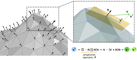
Our choice and use of this extrinsic differential geometry and finite element method approach was aided by the work of many, including refs. [33, 34, 35, 40, 41, 42, 43, 44, 45] and chapter 3 of the supplemental material for [46]. The finite element setting permits us the convenience of carrying out the mathematics in the full three-dimensional setting of $\mathbb{R}^{3}$, while using our knowledge of the normal vectors everywhere on the surface of interest to project our governing equations onto the surface. While velocity is described by the 3-dimensional vector v, both v and the scalar $\rho$ are defined only on the surface. At every point on the surface, derivatives evaluated in the usual $\mathbb{R}^{3}$ way are projected onto the tangent plane using the local normal. For an insightful description of this extrinsic differential geometry approach to handling curved surfaces and its mathematical equivalence to the intrinsic differential geometry strategy, we recommend chapters 22 and 23 of Needham [47]. Central to the extrinsic geometry approach is the projection operator, defined as

$$\mbox{projection onto tangent plane}={\bf P}={\bf I}-{\bf n}\otimes{\bf n},$$

(3)

where ${\bf I}$ is the identity matrix and ${\bf n}\otimes{\bf n}$ is the outer product of the surface normal vector as shown in Figure 2. To make sense of this expression mathematically, we recall that the outer product ${\bf n}\otimes{\bf n}$ is defined through its action on a vector ${\bf v}$ as

$$({\bf n}\otimes{\bf n}){\bf v}={\bf n}({\bf n}\cdot{\bf v}).$$

(4)

We can write ${\bf v}={\bf v}^{\parallel}+{\bf v}^{\perp}$, where ${\bf v}^{\parallel}$ is the component of ${\bf v}$ in the tangent plane of the surface and ${\bf v}^{\perp}$ is normal to the surface. The action of ${\bf I}-{\bf n}\otimes{\bf n}$ on a vector ${\bf v}$ is given by

$$({\bf I}-{\bf n}\otimes{\bf n}){\bf v}={\bf v}-{\bf n}({\bf n}\cdot{\bf v})={\bf v}-{\bf v}^{\perp}={\bf v}^{\parallel},$$

(5)

as illustrated in Figure 2. We can write the projection operator in component form as

$$P_{ij}=\delta_{ij}-n_{i}n_{j},$$

(6)

recalling that the normal vector to the surface is given by ${\bf n}=(n_{1},n_{2},n_{3})$, or in full component form as

$${\bf P}=\left[\begin{array}[]{ccc}1-n_{1}^{2}&-n_{1}n_{2}&-n_{1}n_{3}\\ -n_{1}n_{2}&1-n_{2}^{2}&-n_{2}n_{3}\\ -n_{1}n_{3}&-n_{2}n_{3}&1-n_{3}^{2}\end{array}\right].$$

(7)

Using the projection operator allows us to perform calculations in the ordinary three-dimensional space within which the surface of interest is embedded, but then to pick off only the pieces of the resulting vectors that live within the surface.

In the remainder of this section, we examine each term in the minimal Toner-Tu equations and translate it into its projected form. In Appendix Section 8.1, we define the projected surface form of calculus operators as an additional reference for the reader. First, to modify the preferred speed term to its curved-surface implementation, we note that it is now ${\bf v}^{\parallel}$, the in-plane velocity, that has a privileged magnitude. This magnitude is imposed through the condition

$$\mbox{preferred speed term}=[\alpha(\rho-\rho_{c})-\beta v_{j}^{\parallel}v_{j}^{\parallel}]v_{i}^{\parallel}.$$

(8)

If $|{\bf v}^{\parallel}|$ is either larger or smaller than the privileged value $v_{\mbox{\footnotesize{pref}}}=\sqrt{\alpha(\rho-\rho_{c})/\beta}$, this term will adjust the velocity towards that steady-state magnitude.

Next, we consider the pressure term, whose physical origin comes from a model of pressure in powers of density of the form introduced by Toner and Tu [3],

$$P(\rho)=\sum_{n=1}^{\infty}\sigma_{n}(\rho-\rho_{0})^{n}$$

(9)

where $\rho_{0}$ is the mean density. In the minimal Toner-Tu theory we adopt here, only the first order term in that expansion is kept, with the notational simplification that $\sigma_{1}=\sigma$, resulting in

$$\mbox{pressure term}=-{\partial P\over\partial x_{i}}=-\sigma{\partial\rho\over\partial x_{i}}.$$

(10)

We note that while $\rho_{0}$ is not explicitly present in the gradient of the first order pressure term, for the case considered here of a finite surface on which total density is conserved, this pressure term effectively maintains a density range centered around the mean density $\rho_{0}$ established by our choice of initial condition. The curved-space version of the pressure term requires projecting the full 3D gradient of the density onto the tangent plane, using the projection operator defined in eqn. 3. We follow Jankuhn et al. [34] in introducing the notation $\nabla_{\Gamma}$ for the projected surface gradient operator, where the subscript $\Gamma$ indicates that the gradient is evaluated on the surface of interest. Mathematically, this amounts to computing

$$\nabla_{\Gamma}\rho=({\bf I}-{\bf n}\otimes{\bf n})\nabla\rho,$$

(11)

where $\nabla$ is the ordinary, three-dimensional gradient in Cartesian coordinates. This can be rewritten in component form as

$\displaystyle(\nabla_{\Gamma}\rho)_{i}=\left[({\bf I}-{\bf n}\otimes{\bf n})\nabla\rho\right]_{i}=\left(\delta_{ij}-n_{i}n_{j}\right)\frac{\partial\rho}{\partial x_{j}}=\frac{\partial\rho}{\partial x_{i}}-n_{i}n_{j}\frac{\partial\rho}{\partial x_{j}}.$

(12)

The next term in the Toner-Tu equations that we consider in its curved-space format is the advection term in eqn. 2, namely,

$$\mbox{advection term}=-\lambda v_{j}{\partial v_{i}\over\partial x_{j}}.$$

(13)

In direct notation, the curved-space version of this term has the form

$$\mbox{advection term}=-\lambda({\bf v}^{\parallel}\cdot\nabla_{\Gamma}){\bf v}^{\parallel},$$

(14)

which involves the curved-space version of the velocity gradient tensor. In Appendix Section 8.1, we describe how to compute this tensor, which stated simply is

$$\nabla_{\Gamma}{\bf v}^{\parallel}={\bf P}(\nabla{\bf v}^{\parallel}){\bf P},$$

(15)

where P is the projection operator defined in eqn. 3. In indicial notation, this leads to the result

$$(\nabla_{\Gamma}{\bf v}^{\parallel})_{ij}=[{\bf P}(\nabla{\bf v}^{\parallel}){\bf P}]_{ij}=P_{ik}{\partial v_{k}^{\parallel}\over\partial x_{l}}P_{lj}.$$

(16)

Invoking the definition of the projection operator from eqn. 6, this expression simplifies to the result

$$(\nabla_{\Gamma}{\bf v}^{\parallel})_{ij}=[{\bf P}(\nabla{\bf v}^{\parallel}){\bf P}]_{ij}=\left(\frac{\partial v_{i}^{\parallel}}{\partial x_{j}}-n_{l}n_{j}\frac{\partial v_{i}^{\parallel}}{\partial x_{l}}\right)-n_{i}n_{k}\left(\frac{\partial v_{k}^{\parallel}}{\partial x_{j}}-n_{l}n_{j}\frac{\partial v_{k}^{\parallel}}{\partial x_{l}}\right).$$

(17)

Thus, the curved-space advection term can be written as

$$-\lambda[{\bf P}(\nabla{\bf v}^{\parallel}){\bf P}]_{ij}v_{j}^{\parallel}=-\lambda\left[\left(\frac{\partial v_{i}^{\parallel}}{\partial x_{j}}-n_{l}n_{j}\frac{\partial v_{i}^{\parallel}}{\partial x_{l}}\right)-n_{i}n_{k}\left(\frac{\partial v_{k}^{\parallel}}{\partial x_{j}}-n_{l}n_{j}\frac{\partial v_{k}^{\parallel}}{\partial x_{l}}\right)\right]v_{j}^{\parallel}.$$

(18)

With these examples of tangent-plane calculus established, we now turn to the most tricky of the terms in the Toner-Tu equations, the surface-projected version of the neighbor coupling term, $D\nabla^{2}{\bf v}$. First, we recall that the Laplacian of a vector field in normal 3D Cartesian space is defined as $\nabla^{2}{\bf v}=\nabla\cdot(\nabla{\bf v})$. Further, we note that $\nabla{\bf v}$ is itself a tensor. As shown by Jankuhn et al. [34], the surface-projected version of the Laplacian term (see their eqn. 3.16 for the surface Navier-Stokes equations for the tangential velocity on a stationary surface), is therefore given by

$$\underbrace{\nabla^{2}{\bf v}}_{\mbox{flat Toner-Tu}}=\underbrace{\mbox{div}(\nabla{\bf v})}_{\mbox{in the plane}}~\longrightarrow~~~\underbrace{{\bf P}\mbox{div}_{\Gamma}({\bf G}({\bf v}^{\parallel}))}_{\mbox{curved surface}}.$$

(19)

To begin to unpack this expression, we note that ${\bf P}$ is the projection operator defined in eqn. 3 and that the tensor ${\bf G}$ is the surface velocity gradient,

$${\bf G}({\bf v}^{\parallel})=\nabla_{\Gamma}{\bf v}^{\parallel},$$

(20)

already presented in eqn. 17 and repeated here in component form as

$$G_{ij}=\left(\frac{\partial v_{i}^{\parallel}}{\partial x_{j}}-n_{l}n_{j}\frac{\partial v_{i}^{\parallel}}{\partial x_{l}}\right)-n_{i}n_{k}\left(\frac{\partial v_{k}^{\parallel}}{\partial x_{j}}-n_{l}n_{j}\frac{\partial v_{k}^{\parallel}}{\partial x_{l}}\right).$$

(21)

We note that Jankuhn et al. [34] use a symmetrized version of the velocity gradient since they are deriving the surface versions of the Navier-Stokes equations and are thus taking the divergence of a stress. For the Toner-Tu case of interest here, the “psychological viscosity” that comes from neighboring wildebeest in the herd comparing their velocities is equivalent to the divergence of the velocity gradient itself. We then invoke the definition of the surface-projected divergence of a tensor ${\bf G}$ presented in Appendix Section 8.1, giving rise to a vector of the form

$$\operatorname{div}_{\Gamma}\left({\bf G}\right)_{l}=\frac{\partial G_{lj}}{\partial x_{j}}-n_{j}n_{k}\frac{\partial G_{lj}}{\partial x_{k}}.$$

(22)

We also introduce the shorthand notation for this divergence as

$$\left({\partial G_{lj}\over\partial x_{j}}\right)_{\Gamma}=\frac{\partial G_{lj}}{\partial x_{j}}-n_{j}n_{k}\frac{\partial G_{lj}}{\partial x_{k}}$$

(23)

to simplify some of the complex expressions to follow. Finally, we can write the $i^{th}$ component of the surface version of the Toner-Tu term $D\nabla^{2}{\bf v}$ in indicial notation as

$$D[{\bf P}\mbox{div}_{\Gamma}({\bf G}({\bf v}^{\parallel}))]_{i}=DP_{il}\Big(\frac{\partial G_{lj}}{\partial x_{j}}-n_{j}n_{k}\frac{\partial G_{lj}}{\partial x_{k}}\Big).$$

(24)

We now assemble the results of eqns. 8,  12,  18 and  24 to construct a complete curved-surface formulation of the minimal Toner-Tu equations. Specifically, we have

$${\partial v_{i}^{\parallel}\over\partial t}=[\alpha(\rho-\rho_{c})-\beta v_{j}^{\parallel}v_{j}^{\parallel}]v_{i}^{\parallel}-\sigma\left(\frac{\partial\rho}{\partial x_{i}}-n_{i}n_{j}\frac{\partial\rho}{\partial x_{j}}\right)+DP_{il}\left(\frac{\partial G_{lj}}{\partial x_{j}}-n_{j}n_{k}\frac{\partial G_{lj}}{\partial x_{k}}\right)-\lambda[{\bf P}(\nabla{\bf v}^{\parallel}){\bf P}]_{ij}v_{j}^{\parallel},$$

(25)

which can be streamlined to the alternative form

$${\partial v_{i}^{\parallel}\over\partial t}=[\alpha(\rho-\rho_{c})-\beta v_{j}^{\parallel}v_{j}^{\parallel}]v_{i}^{\parallel}-\sigma\left(\frac{\partial\rho}{\partial x_{i}}\right)_{\Gamma}+DP_{il}\left(\frac{\partial G_{lj}}{\partial x_{j}}\right)_{\Gamma}-\lambda v_{j}^{\parallel}\left[\left({\partial v_{i}^{\parallel}\over\partial x_{j}}\right)_{\Gamma}-n_{i}n_{k}\left({\partial v_{k}^{\parallel}\over\partial x_{j}}\right)_{\Gamma}\right].$$

(26)

Similarly, the curved-space formulation of the governing equation for density can be written as

$$\frac{\partial\rho}{\partial t}=-\frac{\partial(\rho v_{i}^{\parallel})}{\partial x_{i}}+n_{i}n_{j}\frac{\partial(\rho v_{i}^{\parallel})}{\partial x_{j}}=-\left({\partial\rho v_{i}^{\parallel}\over\partial x_{i}}\right)_{\Gamma}.$$

(27)

We now have a complete formulation of our minimal Toner-Tu equations for the general surface context, requiring only a description of the surface in the language of normal vectors. We next turn to the implementation of this general surface formulation in a fashion consistent with finite element treatments on arbitrary surfaces.

To put our finite element formulation into numerical action, we must of course adopt specific values for the parameters $\rho_{0}$, $\rho_{c}$, $\alpha$, $\beta$, $\sigma$, $D$, and $\lambda$ that appear in our governing partial differential equations. In this study, we focus on the macroscopic length scale of animal herds, although we consider the microscopic activity of cytoskeletal proteins elsewhere [27]. While our goal here is to explore the phenomenology of Toner-Tu flocks on curved surfaces in a general way, not to claim an understanding of specific animal behavior, our parameter choices are loosely inspired by migrating wildebeest herds as seen in Figure 3. By inspecting aerial photographs of wildebeest herds, we estimated an average wildebeest density of

$$\rho_{0}=0.25~\mbox{m}^{-2}.$$

(47)

For the critical density above which coordinated herding behavior occurs, we make the estimate

$$\rho_{c}=0.05~\mbox{m}^{-2},$$

(48)

based roughly on the observation that for densities much higher than this, the photographed wildebeest have an organized herd structure. We note that it would be very interesting to carefully measure these parameters in the context of herds of wildebeest with a Toner-Tu framework in mind.

The remainder of the parameters are determined in the spirit of exploring how the different terms compete to alter the density and velocity fields. Thus, parameters are chosen in order to make all the terms comparable in magnitude. We provide here the actual values used in our finite element calculations, fully cognizant that our parameter choices are at best approximate. We begin by estimating the magnitude of $\partial v/\partial t$. We picture wildebeests circling a small hill in the landscape, moving with a characteristic speed of 1 m/s and taking 20 s to change direction completely. This scenario implies

$${\partial v\over\partial t}\approx{1~\mbox{m/s}-(-1~\mbox{m/s})\over 20~\mbox{s}}\approx 0.1~\mbox{m/s}^{2}.$$

(49)

Using the strategy of balancing the magnitudes of the different terms, we estimate the coefficient for the preferred speed terms by considering that

$$0.1~\mbox{m/s}^{2}=\alpha(\rho_{0}-\rho_{c})v\approx\alpha\times(0.25~\mbox{m}^{-2}-0.05~\mbox{m}^{-2})\times 1~\mbox{m/s},$$

(50)

which leads us to adopt

$$\alpha=0.5~\mbox{m${}^{2}$/s}.$$

(51)

For the parameter $\beta$, we choose a value that sets the correct mean field speed, $v_{\mbox{\footnotesize{pref}}}$, for wildebeests. Thus, we adopt

$$\beta=\frac{\alpha\left(\rho_{0}-\rho_{c}\right)}{v_{\mbox{\footnotesize{pref}}}^{2}}\approx\frac{\left(0.5~\mbox{m}^{2}/\mbox{s}\right)\left(0.2~\mbox{m}^{-2}\right)}{(1\mathrm{~m}/\mathrm{s})^{2}}=0.1\mathrm{~s}/\mathrm{m}^{2}.$$

(52)

We can also check independently that the magnitude of the $\beta$ term is of order 0.1 $\mbox{m}/\mbox{s}^{2}$. Indeed,

$$\beta v^{3}\approx 0.1~{\mbox{s}/\mbox{m}^{2}}\times(1~\mbox{m/s})^{3}=0.1~\mbox{m/s}^{2}.$$

(53)

To find the parameter $\sigma$, the coefficient of the pressure term, we consider the gradients in density seen at the edge of a wildebeest herd and estimate that $\rho$ drops from $\rho_{0}=0.25~\mbox{m}^{-2}$ to 0 $\mbox{m}^{-2}$ over 25 m. Using these numbers implies

$$0.1~\mbox{m/s}^{2}=\sigma{\partial\rho\over\partial x}\approx\sigma{0.25~\mbox{m}^{-2}\over 25~\mbox{m}}$$

(54)

which leads us to adopt

$$\sigma=10~\mbox{m}^{4}/\mbox{s}^{2}.$$

(55)

We can now apply this thinking to make an estimate of the neighbor coupling coefficient $D$ by using the equality

$$0.1~\mbox{m/s}^{2}=D{\partial^{2}v\over\partial x^{2}}\approx D{1~\mbox{m/s}\over(10~\mbox{m})^{2}}$$

(56)

which leads to the coefficient choice

$$D=10~\mbox{m}^{2}/\mbox{s}.$$

(57)

To estimate the magnitude of $\lambda$, we imagine that the wildebeest will come to a full stop from a speed of 1 m/s over a distance of roughly 10 m, permitting us to make the correspondence

$$0.1~\mbox{m/s}^{2}=\lambda v{\partial v\over\partial x}\approx\lambda\times 1~\mbox{m/s}\times{1~\mbox{m/s}\over 10~\mbox{m}}$$

(58)

which implies that

$$\lambda=1.$$

(59)

This estimated set of parameters provides us with a complete description of the Toner-Tu herd in the minimal model we seek to explore. Throughout the remainder of the paper, we consistently use these parameter values. In later sections, in some cases we will go beyond this idealized parameter set to perform parameter sweeps that permit different regimes of behavior to emerge. Unless noted otherwise, time-dependent finite element method simulations were initialized with a uniform density field $\rho=\rho_{0}$ and a disordered velocity field, with velocity orientations drawn randomly from a uniform distribution of angles between 0 and 2$\pi$ and with velocity magnitude $v(0)$ = 1 m/s, our estimated characteristic wildebeest speed. We note again that these parameters were chosen to highlight competition between the different terms in the dynamics; they are far from the final word for describing real wildebeest herds.

We next recast the Toner-Tu equations in dimensionless form, rendering the meaning and magnitude of the terms more transparent. For the positional coordinate, we take $x^{*}=x/L$, where $L$ is a characteristic length scale in the problem. In this case, we conceptualize $L$ as the length scale of the wildebeest herd. We note that in the problems considered here, the scale of the herd is the same as the scale of the surface landscape on which the herd moves. Similarly, we use a characteristic velocity scale $U$ to define the dimensionless velocity as $v^{*}=v/U$. We note that $U$ is conceptually related to $v_{\mbox{\footnotesize{pref}}}$, but $v_{\mbox{\footnotesize{pref}}}=\sqrt{\alpha(\rho-\rho_{c})/\beta}$ features a hidden dependence on the density that would complicate our rescaling. Similarly, we can define a dimensionless density $\rho^{*}=\rho/\rho_{c}$, using the critical density $\rho_{c}$ as our scaling variable. Lastly, in light of the definitions above, we can determine a time scale $L/U$, the time it takes for a given wildebeest to cross the entire surface landscape. Thus, we define $t^{*}=t/(L/U)$.

Using the various definitions given above, we can now rewrite the Toner-Tu equations using the dimensionless versions of $t$, $x$, $\rho$ and ${\bf v}$ as

$${U^{2}\over L}{\partial v_{i}^{*}\over\partial t^{*}}=\alpha\rho_{c}U(\rho^{*}-1)v_{i}^{*}-\beta U^{3}|{\bf v}^{*}|^{2}v_{i}^{*}-{\sigma\rho_{c}\over L}{\partial\rho^{*}\over\partial x_{i}^{*}}+{DU\over L^{2}}\nabla_{*}^{2}v_{i}^{*}-{\lambda U^{2}\over L}v_{j}^{*}{\partial v_{i}^{*}\over\partial x_{j}^{*}}.$$

(60)

Dividing everything by $U^{2}/L$ results in five dimensionless parameters whose magnitudes provide a sense of the relative contributions of the different terms, within the full dynamical equations of the form

$${\partial v_{i}^{*}\over\partial t^{*}}={\alpha\rho_{c}L\over U}(\rho^{*}-1)v_{i}^{*}-\beta LU|{\bf v}^{*}|^{2}v_{i}^{*}-{\sigma\rho_{c}\over U^{2}}{\partial\rho^{*}\over\partial x_{i}^{*}}+{D\over UL}\nabla_{*}^{2}v_{i}^{*}-\lambda v_{j}^{*}{\partial v_{i}^{*}\over\partial x_{j}^{*}}.$$

(61)

Using definitions of dimensionless variables given above, we find that the generalized continuity equation takes the form

$${\partial\rho^{*}\over\partial t^{*}}=-{\partial(\rho^{*}v_{i}^{*})\over\partial x_{i}^{*}}.$$

(62)

Next, we briefly turn to interpreting the dimensionless ratios that appear when casting the minimal Toner-Tu theory in dimensionless form as exhibited in eqn. 61. The two components of the preferred speed term have dimensionless parameters given by

$$\mbox{increase to preferred speed parameter}={\alpha\rho_{c}L\over U}={L/U\over 1/(\alpha\rho_{c})}={\mbox{time for wildebeest to cross herd}\over\mbox{time for speed to increase to $v_{\mbox{\footnotesize{pref}}}$ }}$$

(63)

and

$$\mbox{decrease to preferred speed parameter}=\beta LU={L/U\over 1/(\beta U^{2})}={\mbox{time for wildebeest to cross herd}\over\mbox{time for speed to decrease to $v_{\mbox{\footnotesize{pref}}}$}}.$$

(64)

Each of these terms provides intuition about how quickly the wildebeest will return to their steady-state speed given some perturbation that disturbs them from that value. Recall that $L/U$ (the “time for wildebeest to cross herd") is roughly the time it takes for a wildebeest to move a distance equal to the size of the herd, or equivalently, to move across the surface landscape. Put in other words, $L/U$ is the time for density advection across the herd. The pressure term can be rewritten as

$$\mbox{pressure parameter}={\rho_{c}\over U^{2}/\sigma}={\mbox{critical density}\over\mbox{typical density excursion away from $\rho_{0}$ }}.$$

(65)

Increasing $\sigma$ decreases density variance; in other words, densities that emerge are within a more narrow range around the mean density $\rho_{0}$. The neighbor coupling term that carries out democratic velocity smoothing has the dimensionless prefactor

$$\mbox{neighbor coupling parameter}={D\over UL}={L/U\over L^{2}/D}={\mbox{time for wildebeest to cross herd}\over\mbox{time for velocity to diffuse across herd}},$$

(66)

analogous to the Péclet number. The last term can be written as

$$\mbox{advection parameter}={\lambda L/U\over L/U}={\mbox{time for velocity advection across herd}\over\mbox{time for wildebeest to cross herd (density advection)}}.$$

(67)

References

- Pliny [1940] Pliny, Natural History, Volume III, Book 10. Translated by H. Rackham., Harvard University Press, Cambridge, MA, 1940.
- Vicsek et al. [1995] T. Vicsek, A. Czirók, E. Ben-Jacob, I. Cohen, O. Shochet, Novel Type of Phase Transition in a System of Self-Driven Particles, Physical Review Letters 75 (1995) 1226–1229.
- Toner and Tu [1995] J. Toner, Y. Tu, Long-range order in a two-dimensional dynamical XY model: How birds fly together, Physical Review Letters 75 (1995) 4326–4329.
- Toner and Tu [1998] J. Toner, Y. Tu, Flocks, herds, and schools: A quantitative theory of flocking, Physical Review E 58 (1998) 4828–4858.
- Marchetti et al. [2013] M. C. Marchetti, J. F. Joanny, S. Ramaswamy, T. B. Liverpool, J. Prost, M. Rao, R. A. Simha, Hydrodynamics of soft active matter, Reviews of Modern Physics 85 (2013) 1143–1189.
- Ballerini et al. [2008] M. Ballerini, N. Cabibbo, R. Candelier, A. Cavagna, E. Cisbani, I. Giardina, V. Lecomte, A. Orlandi, G. Parisi, A. Procaccini, M. Viale, V. Zdravkovic, Interaction ruling animal collective behavior depends on topological rather than metric distance: Evidence from a field study, Proceedings of the National Academy of Sciences 105 (2008) 1232–1237.
- Woodhouse and Goldstein [2013] F. G. Woodhouse, R. E. Goldstein, Cytoplasmic streaming in plant cells emerges naturally by microfilament self-organization, Proceedings of the National Academy of Sciences 110 (2013) 14132–14137.
- Mayer et al. [2010] M. Mayer, M. Depken, J. S. Bois, F. Jülicher, S. W. Grill, Anisotropies in cortical tension reveal the physical basis of polarizing cortical flows, Nature 467 (2010) 617–621.
- Cavagna and Giardina [2014] A. Cavagna, I. Giardina, Bird flocks as condensed matter, Annual Review of Condensed Matter Physics 5 (2014) 183–207.
- Münster et al. [2019] S. Münster, A. Jain, A. Mietke, A. Pavlopoulos, S. W. Grill, P. Tomancak, Attachment of the blastoderm to the vitelline envelope affects gastrulation of insects, Nature 568 (2019) 395–399.
- Pimpale et al. [2020] L. G. Pimpale, T. C. Middelkoop, A. Mietke, S. W. Grill, Cell lineage-dependent chiral actomyosin flows drive cellular rearrangements in early Caenorhabditis elegans development, eLife 9:e54930 (2020) 1–35.
- Wioland et al. [2016] H. Wioland, F. G. Woodhouse, J. Dunkel, R. E. Goldstein, Ferromagnetic and antiferromagnetic order in bacterial vortex lattices, Nature Physics 12 (2016) 341–345.
- Bricard et al. [2013] A. Bricard, J. B. Caussin, N. Desreumaux, O. Dauchot, D. Bartolo, Emergence of macroscopic directed motion in populations of motile colloids, Nature 503 (2013) 95–98.
- Kumar et al. [2014] N. Kumar, H. Soni, S. Ramaswamy, A. K. Sood, Flocking at a distance in active granular matter, Nature Communications 5 (2014).
- Sanchez et al. [2012] T. Sanchez, D. T. N. Chen, S. J. DeCamp, M. Heymann, Z. Dogic, Spontaneous motion in hierarchically assembled active matter., Nature 491 (2012) 431–434.
- Morin et al. [2017] A. Morin, N. Desreumaux, J. B. Caussin, D. Bartolo, Distortion and destruction of colloidal flocks in disordered environments, Nature Physics 13 (2017) 63–67.
- Souslov et al. [2017] A. Souslov, B. C. Van Zuiden, D. Bartolo, V. Vitelli, Topological sound in active-liquid metamaterials, Nature Physics 13 (2017) 1091–1094.
- Wu et al. [2017] K. T. Wu, J. B. Hishamunda, D. T. Chen, S. J. DeCamp, Y. W. Chang, A. Fernández-Nieves, S. Fraden, Z. Dogic, Transition from turbulent to coherent flows in confined three-dimensional active fluids, Science 355 (2017).
- Shankar et al. [2020] S. Shankar, A. Souslov, M. J. Bowick, M. Cristina Marchetti, V. Vitelli, Topological active matter, arXiv 2010.00364 (2020) 1–20.
- Zhang et al. [2020] B. Zhang, B. Hilton, C. Short, A. Souslov, A. Snezhko, Oscillatory chiral flows in confined active fluids with obstacles, Physical Review Research 2 (2020) 43225.
- Behrndt et al. [2012] M. Behrndt, G. Salbreux, P. Campinho, R. Hauschild, F. Oswald, J. Roensch, S. W. Grill, C.-p. Heisenberg, Forces Driving Epithelial Spreading in Zebrafish Gastrulation, Science 338 (2012) 257–260.
- Streichan et al. [2018] S. J. Streichan, M. F. Lefebvre, N. Noll, E. F. Wieschaus, B. I. Shraiman, Global morphogenetic flow is accurately predicted by the spatial distribution of myosin motors, eLife 7:e27454 (2018).
- Maroudas-Sacks et al. [2021] Y. Maroudas-Sacks, L. Garion, L. Shani-Zerbib, A. Livshits, E. Braun, K. Keren, Topological defects in the nematic order of actin fibres as organization centres of Hydra morphogenesis, Nature Physics 17 (2021) 251–259.
- Cicconofri et al. [2020] G. Cicconofri, M. Arroyo, G. Noselli, A. DeSimone, Morphable structures from unicellular organisms with active, shape-shifting envelopes: Variations on a theme by Gauss, International Journal of Non-Linear Mechanics 118 (2020).
- Pearce et al. [2020] D. J. G. Pearce, S. Gat, G. Livne, A. Bernheim-Groswasser, K. Kruse, Programming active metamaterials using topological defects, arXiv 2010.13141 (2020) 1–8.
- Hoffmann et al. [2023] L. A. Hoffmann, L. N. Carenza, L. Giomi, Tuneable defect-curvature coupling and topological transitions in active shells, Soft Matter 19 (2023).
- Hueschen et al. [2022] C. L. Hueschen, L. Segev Zarko, J.-H. Chen, M. A. Le Gros, C. A. Larabell, J. C. Boothroyd, R. Phillips, A. R. Dunn, Emergent actin flows explain diverse parasite gliding modes, bioRxiv (2022).
- Toner et al. [2005] J. Toner, Y. Tu, S. Ramaswamy, Hydrodynamics and phases of flocks, Annals of Physics 318 (2005) 170–244.
- Bowick et al. [2022] M. J. Bowick, N. Fakhri, M. C. Marchetti, S. Ramaswamy, Symmetry, Thermodynamics, and Topology in Active Matter, Physical Review X 12 (2022) 10501.
- Scriven [1960] L. E. Scriven, Dynamics of a fluid interface: Equation of motion for Newtonian surface fluids, Chemical Engineering Science 12 (1960) 98–108.
- Fily et al. [2016] Y. Fily, A. Baskaran, M. F. Hagan, Active Particles on Curved Surfaces, arXiv 1601.00324 (2016) 1–9.
- Nitschke et al. [2017] I. Nitschke, S. Reuter, A. Voigt, Discrete exterior calculus (DEC) for the surface Navier-Stokes equation, Advances in Mathematical Fluid Mechanics: Transport Processes at Fluidic Interfaces (2017).
- Sahu et al. [2017] A. Sahu, R. A. Sauer, K. K. Mandadapu, Irreversible thermodynamics of curved lipid membranes, Physical Review E 96 (2017) 45–47.
- Jankuhn et al. [2018] T. Jankuhn, M. A. Olshanskii, A. Reusken, Incompressible fluid problems on embedded surfaces: Modeling and variational formulations, Interfaces and Free Boundaries 20 (2018) 353–378.
- Mietke et al. [2019] A. Mietke, F. Jülicher, I. F. Sbalzarini, Self-organized shape dynamics of active surfaces, Proceedings of the National Academy of Sciences 116 (2019) 29–34.
- Torres-Sanchez et al. [2019] A. Torres-Sanchez, D. Millan, M. Arroyo, Modelling fluid deformable surfaces with an emphasis on biological interfaces, Journal of Fluid Mechanics 872 (2019) 218–271.
- Toner [2018] J. Toner, Why walking is easier than pointing: Hydrodynamics of dry active matter, Active Matter and Nonequilibrium Statistical Physics: Lecture Notes of the Les Houches Summer School: Volume 112 (2022) 1–54.
- Dadhichi et al. [2020] L. P. Dadhichi, J. Kethapelli, R. Chajwa, S. Ramaswamy, A. Maitra, Nonmutual torques and the unimportance of motility for long-range order in two-dimensional flocks, Physical Review E 101 (2020) 1–13.
- Shankar et al. [2017] S. Shankar, M. J. Bowick, M. C. Marchetti, Topological sound and flocking on curved surfaces, Physical Review X 7 (2017).
- Mietke [2018] A. Mietke, Dynamics of active surfaces, Ph.D. Dissertation, TU Dresden (2018).
- Nestler et al. [2018] M. Nestler, I. Nitschke, S. Praetorius, A. Voigt, Orientational Order on Surfaces: The Coupling of Topology, Geometry, and Dynamics, Journal of Nonlinear Science 28 (2018) 147–191.
- Fries [2018] T. P. Fries, Higher-order surface FEM for incompressible Navier-Stokes flows on manifolds, International Journal for Numerical Methods in Fluids 88 (2018) 55–78.
- Nestler et al. [2019] M. Nestler, I. Nitschke, A. Voigt, A finite element approach for vector- and tensor-valued surface PDEs, Journal of Computational Physics 389 (2019) 48–61.
- Nitschke et al. [2019] I. Nitschke, S. Reuther, A. Voigt, Hydrodynamic interactions in polar liquid crystals on evolving surfaces, Physical Review Fluids 4 (2019).
- Rangamani et al. [2013] P. Rangamani, A. Agrawal, K. K. Mandadapu, G. Oster, D. J. Steigmann, Interaction between surface shape and intra-surface viscous flow on lipid membranes, Biomechanics and Modeling in Mechanobiology 12 (2013) 833–845.
- Takatori and Mandadapu [2020] S. C. Takatori, K. K. Mandadapu, Motility-induced buckling and glassy dynamics regulate three-dimensional transitions of bacterial monolayers, arXiv 2003.05618 (2020).
- Needham [2020] T. Needham, Visual Differential Geometry and Forms, Princeton University Press, Princeton, NJ, 2020.
- Curtin et al. [2018] N. A. Curtin, H. L. Bartlam-Brooks, T. Y. Hubel, J. C. Lowe, A. R. Gardner-Medwin, E. Bennitt, S. J. Amos, M. Lorenc, T. G. West, A. M. Wilson, Remarkable muscles, remarkable locomotion in desert-dwelling wildebeest, Nature 563 (2018) 393–396.
- Wu [2021] Z. Wu, Counting Wildebeest From Space Using Deep Learning, Ph.D. Dissertation, University of Twente (2021).
- Morin and Bartolo [2018] A. Morin, D. Bartolo, Flowing Active Liquids in a Pipe: Hysteretic Response of Polar Flocks to External Fields, Physical Review X 8 (2018) 21037.
- Sknepnek and Henkes [2015] R. Sknepnek, S. Henkes, Active swarms on a sphere, Physical Review E 91 (2015) 1–13.
- Kamien et al. [2009] R. D. Kamien, D. R. Nelson, C. D. Santangelo, V. Vitelli, Extrinsic curvature, geometric optics, and lamellar order on curved substrates, Physical Review E 80 (2009).
- Green et al. [2017] R. Green, J. Toner, V. Vitelli, Geometry of thresholdless active flow in nematic microfluidics, Physical Review Fluids 2 (2017) 20–24.
- COMSOL Multiphysics [2017] COMSOL Multiphysics, The Finite Element Method (FEM), Multiphysics Cyclopedia, https://www.comsol.com/multiphysics/finite-element-method, 2017.