Invertible Neural Networks for Graph Prediction
Abstract
Graph prediction problems prevail in data analysis and machine learning. The inverse prediction problem, namely to infer input data from given output labels, is of emerging interest in various applications. In this work, we develop invertible graph neural network (iGNN), a deep generative model to tackle the inverse prediction problem on graphs by casting it as a conditional generative task. The proposed model consists of an invertible sub-network that maps one-to-one from data to an intermediate encoded feature, which allows forward prediction by a linear classification sub-network as well as efficient generation from output labels via a parametric mixture model. The invertibility of the encoding sub-network is ensured by a Wasserstein-2 regularization which allows free-form layers in the residual blocks. The model is scalable to large graphs by a factorized parametric mixture model of the encoded feature and is computationally scalable by using GNN layers. The existence of invertible flow mapping is backed by theories of optimal transport and diffusion process, and we prove the expressiveness of graph convolution layers to approximate the theoretical flows of graph data. The proposed iGNN model is experimentally examined on synthetic data, including the example on large graphs, and the empirical advantage is also demonstrated on real-application datasets of solar ramping event data and traffic flow anomaly detection.
1 Introduction
Graph prediction is an important topic in statistics, machine learning, and signal processing, and is motivated by various applications, e.g., protein-protein interaction networks [45], wind power prediction [46], and user behavior modeling in social networks [7]. There can be various versions of graph prediction problems. We are interested in the scenario where one observes nodal (multi-dimensional) features , nodal responses , and graph topology information. The prediction algorithm typically will then leverage graph topology information to facilitate the learning of predicting given . In practice, Graph Neural Network (GNN) models [44] have become a popular choice due to their expressiveness power and scalable computation. In the so-called inverse of a graph prediction problem, one would like to infer the input graph nodal features given an outcome response . Such a problem is of interest in various real-world applications, for instance, in molecular design [36], scientists want to infer features of the molecule that lead to certain outcomes; in power outage analysis [48, 1], we are interested in finding features (e.g., weather or past power output by sensors) that leads to outages for future prevention. The inverse graph prediction problem is the focus of the current work, for which we develop an invertible deep model that can be efficiently applied to graph data.
The prediction and inverse prediction problems are illustrated in Fig. 1. The left plot shows the case of general non-graph data, and the right plot shows the case with graph data and graph label . As an illustrative example, suppose the graph is a power grid, where each node denotes a power generator, denotes historical power outputs from generator , and denotes the status of the generator (e.g., for functioning normally, and 1 for anomaly). For system monitoring, it is useful to predict the status of generators given historical observations (the forward prediction, indicated by solid black arrows), as well as to generate unobserved possible circumstances given generator status (the inverse, indicated by dashed black arrows) for cause analyses.
To formalize the notion of inverse prediction, we adopt some probability terminologies. The forward prediction problem is to predict from input , which can be formulated as learning the conditional probability of . The inverse prediction problem is to learn the conditional probability of and to generate samples from it. Note that a discriminative task seeks to estimate the posterior at a given (test) point , which can be done by a conventional classification model. The generative task is different in that one asks to sample according to , that is, given a label , to produce samples which do not exist in the training data nor any provided test set. The problem is challenging when data is in high dimensional space, where a grid of can not be efficiently constructed. In particular, when is graph nodal feature data, the dimensionality of scales linearly with the graph size (the number of nodes in the graph). In the case of categorical response, the graph label assigns one of the -class labels to each node, which makes the total possible outcomes many. Thus the inverse prediction problem on graph data poses both modeling and computational challenges when scalability to large graphs is needed.

In this work, we develop a deep generative model for the conditional generation task of the inverse prediction problem on graphs. While deep generative models like generative adversarial networks (GAN) [15, 19], variational auto-encoders (VAE) [25, 26] and normalizing flow networks [27] have been intensively developed in recent years, the conditional generation task given categorial prediction labels is less studied. We further review the literature and comment on related works in Section 2.1. Unlike previous conditional generative models [32, 21, 3, 4, 2], which typically concatenate the prediction label with the random code as input or rely on curated forms of neural network (NN) layers to ensure invertibility, we propose to encode the input data one-to-one by an invertible network to an intermediate feature , from which the label can be predicted using a linear classifier, and in the other direction can also be generated from by a parametric mixture model. The framework of our model is shown in Fig. 2. Because the general (non-graph) data case can be seen as a special case of graph data where the graph only has one node, we call the proposed model invertible Graph Neural Network (iGNN), as a unified name.
To efficiently handle the up to exponentially many outcomes of graph nodal labels, we introduce a factorized mixture distribution over graphs. We theoretically show that the capacity to learn the conditional distribution over a graph can be achieved when the per-node Gaussian mixture model has well-separated components, and the need separation increases with graph size only mildly (an additive factor), cf. Proposition 3.2. Under this formulation, the -to- sub-network is light in model and computation. The major part of the model capacity of the iGNN model is in the -to- sub-network, which is an invertible flow model based on Residual Network (ResNet) framework [5]. The computational scalability to large graphs is tackled by adopting GNN layers, which are not compatible with normalizing flow models having constrained formats in architecture [14, 43], and would also complicate the spectral normalization technique in [5] to ensure network invertibility.
To overcome these issues, we propose Wasserstein-2 regularization of the ResNet, which in the limit of a large number of residual blocks recovers the transport cost in the dynamic formulation of optimal transport (OT) [41, 6, 42]. Based on known results of OT theory, the Wasserstein-2 regularization leads to smooth trajectories of the transported densities. The invertibility of the induced flow map can then be guaranteed with a sufficient number of residual blocks. We empirically verify the invertibility of the flow model in experiments. This allows our model to use free-form neural network layers inside the ResNet blocks, including any GNN layer types. Theoretically, we study the existence and invertibility of flow mapping based on theories of OT and diffusion process. We also prove the expressiveness of GNN layers to approximate the velocity field in the theoretical flows when data is a Gaussian field on the graph.
We examine the performance of the proposed iGNN model on simulated graph data as well as data from real-world graph prediction applications. In summary, the contributions of the work are
We propose a two-step procedure, -to- and -to-, to tackle the generative task of inverse prediction problem viewed as a conditional generation problem and develop an invertible flow model consisting of two subnetworks accordingly. The model is made scalable to graph data by a factorized formulation of the parametric mixture model and the GNN layers in the invertible flow network between and .
We introduce Wasserstein-2 regularization of the invertible flow network, which is computationally efficient and compatible with general free-form layer types, particularly the GNN layers in the flow model. The effect on preserving invertibility is backed by OT theory and verified in practice.
The existence of invertible flow maps is analyzed theoretically. Based on the theoretical flows, we analyze the expressiveness of spectral and spatial graph convolution layers applied to graph data.
The proposed iGNN model is applied to both simulated and real-data examples, showing improved generative performance over alternative conditional generation models.
Notation. We denote by the integer set. denotes the expectation over , that is, . When a probability distribution has density, we use the same notation, e.g., , to denote the distribution and the density. For real-diagonalizable matrix , and function , we denote by the function of the matrix . For and a distribution on , we denote by the push-forward of distribution by , i.e., .
2 Background
2.1 Related works
Generative deep models and normalizing flow. At present, generative adversarial networks (GAN) [15, 19] and variational auto-encoders (VAE) [25, 26] are two of the most popular frameworks that have achieved various successes [31, 47, 28]. However, they also suffer from clear limitations such as notable difficulties in training, such as mode collapse [35] and posterior collapse [30]. On the other hand, normalizing flows (see [27] for a comprehensive review) estimate arbitrarily complex densities via the maximum likelihood estimation (MLE), and they transport original random features into distribution that are easier to sample from (e.g., standard multivariate Gaussian) through invertible neural networks. Flow-based models can be classified into two broad classes: the discrete-time models (some of which include coupling layers [14], autoregressive layers [43] and residual networks [5, 10]), and the continuous-time models as exemplified by neural ODE [17, 33]. Most normalizing flow methods focus on unconditional generation with little development in a conditional generation. In addition, to achieve numerically reliable training, regularization of the density transport trajectories in flow networks are necessary but remain a challenge. In this work, we propose Wasserstein-2 regularization motivated by the transport cost in the dynamic formula of optimal transport (OT) theory. In Remark 2, we compare with the original spectral normalization in iResNet [5] in more detail.
Conditional generation networks. The conditional generation versions of GAN (cGAN) have been studied in several places [32, 21], where the prediction outcome (one-hot encoded as ) are typically concatenated with random noise and taken as input to the generator network, as illustrated in the left of Fig. 2. The one-hot encoding of categorical concatenated with Gaussian poses challenges in training cGAN models, in addition to known issues of their unconditional counterparts, such as mode collapse, posterior collapse, and failures to provide exact data likelihood. When the prediction label is lying on a graph having nodes, the one-hot coding will increase up to more coordinates to the input , which significantly increases the model complexity and computational load with large graphs. Conditional invertible neural network (cINN) model was developed in [3] for analyzing inverse problems. The model inherits the approach of cGAN models to concatenate one-hot encoded prediction label with normal code while using Real-NVP layers [14] to ensure neural network invertibility. In terms of training objective, [3] proposed to use maximum mean discrepancy (MMD) losses to encourage both the matching of the input data distribution and the independence between label and normal code . We call the method in [3] cINN-MMD. Replacing the MMD losses with a flow-based objective, [4, 2] extended the invertible network approach in [3] and applied to image generation problems. In the models in [4] and [2], which we call cINN-Flow and cINN-Flow+ respectively, the inputs to the Real-NVP layers contain encoded information of the prediction label so as to learn label-conditioned generation, see more in Fig. A.1. In experiments, we compare with cGAN and cINN models on both non-graph and graph data.
2.2 Transport cost regularization
We review needed background on the transport cost and the dynamic formula of Wasserstein-2 optimal transport (OT). The transport cost has been proposed to regularize the normalizing flow neural network models, e.g., in [33]. Consider the trajectory satisfying , that is, is the velocity field, where and . The transport cost is defined as
| (1) |
where is the marginal distribution of after pushing forward the initial distribution by for time . The cost (1) can be viewed as taking the kinetic energy in computing the Lagrangian action along the trajectory. A more general form of cost under the framework of Mean-field Games has been proposed in the current and independent work [20] to regularize trajectories of normalizing flows. It is also known that minimizing the cost under the constraint of transporting from fixed to leads to the dynamic formulation of OT, i.e., the Benamou-Brenier formula [41, 6]. Specifically, the solution of the minimization
| (2) |
recovers the Wasserstein-2 OT from to , that is, at the minimizer , and . The minimizer of (2) can be interpreted as the optimal control of the transport problem from to .
In terms of neural network implementation, OT-Flow [33] used the potential model based on OT theory and parametrized the potential by a neural network, where gives the velocity . Our method adopts a ResNet base model, where the invertibility is fulfilled by a Wasserstein-2 regularization, which can be viewed as a finite-step discrete-time counterpart of the transport cost . The proposed Wasserstein-2 regularization recovers with a large number of steps, yet does not require integrating the continuous-time flow with accuracy for all time, cf. Remark 3.
3 Methods
Given data-label pairs , we first describe our approach when is a sample in , and is the categorical label in classes, i.e., . The case where both and lie on a graph is addressed in Section 3.3 where we make the approach scalable to large graphs. In Section 3.4, we introduce Wasserstein-2 regularization to preserve the invertibility of the trained flow network with free-form residual block layer types. All proofs are in Appendix A.
3.1 Inverse of prediction as conditional generation
The overall framework is to (end-to-end) train a network consisting of two sub-networks: the first sub-network maps invertibly from to an intermediate representation , and the second sub-network maps from to label , which is a classifier and loses information. Specifically,
- classification sub-network. We model by a Gaussian mixture model with “well-separated” means (detailed in Section 3.2). The parametric form of contains trainable parameter , and the generation of is by sampling the corresponding mixture component accordingly. The prediction of label from can be conducted by a linear classifier parametrized by . The trainable parameters in the classification sub-network are denoted as .
- invertible sub-network. The invertible mapping from to is by a flow ResNet in (detailed in Section 3.4). The sub-network parameters are denoted as , where is the number of residual blocks, and the network mapping is denoted as . The prediction of label from input is by first computing and then applying the -to- classifier sub-network parametrized by . The generation of is by inversely mapping once is sampled according to parametrized by .
Remark 1 (Encoding-decoding perspective).
The design of the network can be regarded as an encoding scheme that maps to , and in the encoded domain are “noisy codes” represented by separable isotropic Gaussian that can be linearly classified and generated (through the - sub-network). In this sense, the invertible neural network can be viewed as an invertible encoder that preserves information content of in the encoding domain .
The end-to-end training objective of the proposed network can be written as
| (3) |
where , and are the generative loss, the classification loss and the Wasserstein-2 regularization, respectively. The scalars are penalty factors. We will explain the choice of later in this subsection, and the choice of is explained after the derivation in Section 3.4.
Given many data-label pairs , the generative loss is defined as where
| (4) |
Because is a mixture model parametrized by , the per-sample loss is determined by both and . We specify the construction and training of in Section 3.2. The mapping is by an invertible ResNet. The construction of , including the computation of and the regularization loss , will be explained in Section 3.4.
Finally, the classification loss is defined as , where is the per-sample -class classification cross-entropy loss computed by softmax. We use a linear classifier to predict given , parametrized by . When is close in distribution to the Gaussian mixture model specified by , one may also use to construct the linear classifier from to , that is, to tie the parameters and . Here we separately parametrize the forward and inverse prediction parameters in - sub-network so as to facilitate optimization since, in both directions, the model is light. For the penalty factor , we find the experimental results insensitive to the choice. We use in all experiments.


3.2 Mixture model of and the shared flow
We parametrize by a Gaussian mixture model as
| (5) |
where is a prefixed parameter. The mean vectors will be trainable, and we use isotropic Gaussian with the same covariance matrix for simplicity, which may be generalized. Note that we only parametrize the locations of means of the Gaussian components, and there is no need to specify the weights (fraction of samples in each component) because the fractions will be determined by the data. Fig. 3 provides an example where the fractions in the three classes differ.
We will initialize and train the mean vectors to be sufficiently separated to ensure the Gaussian components have almost non-overlapping supports. Formally, we say that a collection of objects in are -separated if for any two distinct elements , . When is a collection of points in , , then . When is a collection of sets in , and , we define . A set is called an -support of a probability distribution if . When the means of Gaussian components are sufficiently separated, one would expect that there are -supports of the components that are mutually separated. Technically, we have that -separation of the means guarantees -mutual separation of -supports, where . The formal statement is proved in the following lemma.
Lemma 3.1 (Separation of components).
Let for . If the mean vectors of the Gaussian mixture distribution of are -separated in , then each component in (5) has an -support such that for , .
The separation condition of the mixture model, especially the high dimensional counterpart in Proposition 3.2, may potentially be connected to the coding theory of Gaussian channel [40]. We further comment on this in the discussion section. The purpose of having separated -supports of the components in is for the construction of an invertible flow map from to that transports each class of samples correspondingly. Intuitively, the separated -supports of the components of allow to partition into domains with smooth boundary where each domain contains . If the -class distributions also have separated -supports , then one can try to construct an invertible flow mapping in which transports to by transporting from to respectively. While the transport from each to can be constructed individually, the simultaneous transports of the components by a shared flow would need the transported components to stay separated from each other along the flow, and this may not always be possible, e.g., due to topological constraints. For the shared invertible flow to exist, we introduce the following assumption:
Assumption 1 (Shared flow).
There exist and constant such that for any , if the components of the Gaussian mixture of have -supports which are mutually -separated in , then there exists a smooth invertible flow mapping induced by velocity field for (i.e. from , and solves the ODE of ) such that the transported conditional distributions satisfy that for .
While theoretical justification of Assumption 1 goes beyond the scope of the paper and is postponed here, we demonstrate the validity of the assumption empirically. An example of the shared invertible flow on a 3-class data in is illustrated in Fig. 3. In all our experiments, we find that the trained invertible ResNet successfully transports from to for all classes. In the special case of having class, the conditional generation problem reduces to an unconditional one and the shared flow is no longer an issue. In this case, one can set the distribution of to be a standard normal, and the desired transport map is a normalizing flow. In Section 4 we further study the existence and theoretical properties of the flow mapping when , for general data and graph data.
Assumption 1 guarantees the existence of a shared flow mapping which transports the -class conditional densities up to error as long as the components of the Gaussian mixture distribution have -separated -supports. Meanwhile, by Lemma 3.1, will have -separated -supports if the means are separated as therein. Since , it will exceed the constant required by Assumption 1 when is small. This suggests keeping the mean vectors to be separated at the order of . In practice, we initialize to be separated at such a scale and preserve the separation during training via a barrier penalty on the distances .
3.3 Scalable conditional generation on graph data
The mixture modeling of described in the previous section is scalable to large graphs, as we explain in this subsection. Consider the graph data where both the data vector and the label are defined on each node in a graph. In this subsection, the subscript v indicates graph node . Suppose the graph has nodes in , and the edge set is specified by an adjacency matrix . We denote a graph data sample and a graph label as , , , , , where is the dimension of node feature. One may view as a vector in , , and label vector taking many possibilities, and then apply the approach for non-graph data to the -class prediction problem in . However, this may lead to exponentially many classes when the graph size is large, leading to difficulty in modeling by a mixture distribution as well as large model complexity.
To make our approach scalable to large graphs, we adopt two techniques: (i) we introduce a factorized form of which is independent and homogeneous over graph; (ii) we propose to use GNN layers in the invertible flow ResNet, which makes the neural network computation scalable. The scalability of our iGNN approach is demonstrated on a larger graph with nodes, cf. Fig. 5.
(i) Factorized over graph. Recall that is of same dimension as and also defined on ,
Suppose we have a -component Gaussian mixture distribution of means in , we specify the graph as
| (6) |
that is, the joint distribution of consists of independent and identical -component Gaussian mixture distribution of in across the graph. As a result, on the graph sample-label pair , the term in the generative loss (4) can be computed as
| (7) |
where is specified by a Gaussian mixture model in .
The factorized form of reduces the complexity of modeling in to that of modeling a -class mixture model in . At the same time, one would prefer that such a reduction does not prevent the mixture distribution from presenting any sufficiently separated conditional distribution via an invertible mapping in . Under Assumption 1, the desired shared flow in exists as long as the -separation between some -supports of the components of can be achieved. Due to that is ( is concatenated from , ), and the length of is of order , this raises the question of how the separation of the Gaussian means of in needs to scale with large . The following proposition shows that, theoretically, compared to Lemma 3.1 only an additional separation is needed.
Proposition 3.2 (Separation of components).
Let for . If the mean vectors of the Gaussian mixture distribution of are -separated in , then the components of the Gaussian mixture distribution of in satisfy that each component has an -support and for any , .
The proposition suggests that the needed separation of Gaussian mixture means in increases mildly when the graph size increases. In experiments, we find that using the same algorithmic setting to preserve mean vectors’ separation in suffices for graph data experiments where is up to a few hundreds.
(ii) Scalable computation on the graph. As will be introduced in Section 3.4, the residual block in the proposed iGNN model can take a general form (the invertibility will be enforced by a Wasserstein transport regularization). This allows using any GNN layer type in the residual block, which can be made computationally scalable to large graphs [44].
Consider input graph data in , where is the number of nodes, and is the dimension of node features. We denote by the output graph data in after the graph convolution, and we adopt spectral and spatial graph convolution layers in this work. Because and can be hidden-layer features inside the residual block, the dimension and may be larger than the data node feature dimension . Let be the graph Laplacian matrix, possibly normalized so that the spectrum lines on a unit interval. Omitting the bias term and the non-linear node-wise activation function, the GNN layers used in this work are
ChebNet [13], where , parametrized by , and is the Chebyshev polynomial of degree .
L3Net [11], where , parametrized by which are local filters on graph and .
The benefit of using GNN layer lies in the reduced model and computational complexities: the number of trainable parameters in a ChebNet layer is , and that in an L3Net layer is where denotes average local patch size [11]. In contrast, a fully-connected layer mapping from to would have many parameters, which is not scalable to large graphs. We include the fully-connected layer baseline in experiments when the graph size is small and compare performance with the GNN layers.
3.4 Invertible flow network with Wasserstein-2 regularization
We use an invertible flow network to construct the encoding which maps one-to-one between and . The base model follows the framework of [5]. The ResNet has residual blocks, and the -th block residual mapping is parametrized by . The overall ResNet mapping from to can be expressed as where
| (8) |
In each of the residual blocks, we use a shallow network with one or two hidden layers for . The parameter consists of the weights and bias vectors of the shallow network. The ResNet architecture is illustrated on the right of Fig. 2. The architecture of the residual block is free-form: one can use any layer type inside the residual blocks and even different layer types in different blocks. In this work, we use a fully-connected layer for Euclidean data and GNN layers for graph data. To compute the log determinant in (4), we express the quantity as a power series and adopt the technique in [10] to obtain an unbiased estimator. Further details can be found in Appendix B.1.
The invertibility of the ResNet is to be fulfilled by using sufficiently large together with the Wasserstein-2 regularization in (3), which we introduce here. The regularization takes the form as
where and is defined as in (8). Replacing the empirical measure of training samples by the data density gives the population counterpart of as . We denote by the transport map from to , that is,
| (9) |
and then . Define the composite of ’s as , which is the transport mapping from to , namely, , , for , and . We also define which is the marginal distribution of , and . Then can be equivalently written as
| (10) |
We will show in Section 4.1 that regularizing by is equivalent to adding
to the minimizing objective. We thus call the proposed regularization the “Wasserstein-2 regularization,” because sums over the step-wise (squared) Wasserstein-2 distance over the steps.
In the limit of large , the proposed regularization by serves to penalize the transport cost. When , the optimal flow induced by the minimizer gives the Wasserstein geodesic from to the normal density, cf. Section 4.2. In our problem of conditional generation, when there are classes, the limiting continuous time flow differs from the Wasserstein geodesic from to for fixed , but is expected to give a shared flow in from to , cf. Assumption 1 and Fig. 3. Under regularity conditions, one would expect the transport-cost regularized continuous-time flow to also be regular (the case is proved in Proposition 4.2). As a result, the velocity field would have a finite -Lipschitz constant on any bounded domain. Then, the transport from to induced by on the interval is invertible when , which holds when . In this case, also assuming that the solved discrete-time transport map is close to that induced by , one can expect the invertibility of to hold for each , and then the composed transport is also invertible.
We numerically verify the invertibility of the trained in ResNet in experiments, cf. Table 1 and Appendix B. Our analysis in Section 4.1 also suggests that the regularization factor should scale with , the number of residual blocks. In experiments, we find that the invertibility of the ResNet can be guaranteed over a range of choices of , and the quality of generation is insensitive to the choice, see more in Appendix B.3. The number of blocks to use depends on the complication of the data distribution, and in all our experiments, we find a few tens to be enough, including the large graph experiment.
Remark 2 (Comparison to spectral normalization).
iResNet [5] proposed spectral normalization to ensure the invertibility of each residual block. Given a weight matrix in a fully-connected layer, the method first computes an estimator of the spectral norm by power iteration [16], and then modify the weight matrix to be if , where is a pre-set scaling parameter. It was proposed to apply the procedure to all weight matrices in all ResNet blocks in every stochastic gradient descent (SGD) step with mini-batches. When the number of blocks is large, this involves expensive computation, especially if the hidden layers are wide, i.e., and being large. In addition, while spectral normalization of fully-connected layers together with contractive nonlinearities (e.g., ReLU, ELU, Tanh) ensures invertibility, it may not be directly applicable to other layer types, e.g., GNN layers. In contrast, the proposed Wasserstein-2 regularization are obtained from the forward passes of the residual blocks on mini-batches of training samples without additional computation. It is also generally compatible with free-form neural network layer types.
4 Theory: Invertible flow
In this section, we first interpret the proposed Wasserstein-2 regularization in view of transport cost in Section 4.1. In Section 4.2, utilizing theories of diffusion process and the dynamic formulation of OT, we theoretically study the existence of invertible flow in the simplified case where . All proofs are in Appendix A.
Throughout the section, we consider flow mapping induced by a velocity field , that is, the continuous-time flow is represented by an initial value problem (IVP) of ODE
| (11) |
The transport in is the solution mapping from to at some time .
4.1 Interpretation of Wasserstein-2 regularization
The proposed regularization by in Section 3.4 can be interpreted using the dynamic formula of the Wasserstein-2 transport, where we recall the notations in Section 2.2. Suppose the time interval is divided into time steps, . With the optimal velocity field and the corresponding that minimize the transport cost in (2), on every time subinterval , . By the definition of the transport cost (1), we have
| (12) |
Note that the right hand side (r.h.s.) only depends on at the time stamps . We define , and denote by the transport map from to induced by the ODE of on the time interval , i.e., starting from . About the notation, and here are determined by the continuous-time flow, and the notations coincide with those in (9) and (10) which are determined by the finite-step ResNet. We use the same notations here since will be the variables to minimize the training objective, and thus ready to be parametrized by a residual block .
Specifically, when the other part in the loss, denoted as , only depends on the terminal time density , one can use the r.h.s. of (12) as the regularization term added to , making the overall objective as
| (13) |
where , . Note that for a given , the densities are determined by the transport maps ’s, this means that can be used as the variables to minimize (13).
The following proposition shows that this minimization is equivalent to using the proposed Wasserstein-2 regularization in Section 3.4 (specifically, using times the r.h.s. of (10)) in solving for ’s, and there is no need to solve for the OT distance with additional computation.
Proposition 4.1 (Equivalent form of ).
Minimizing (13) over is equivalent to
| (14) |
Remark 3.
The regularization (10) can also be viewed as a first-order approximation of the transport cost (1) using the Forward Euler scheme, that is, by (replacing the integral with finite summation at and) the approximation that . Note that our derivation is based on (13), which coincides with the continuous-time transport cost in the limit of large , but is well-defined for finite . The objective (13) only involves the discrete-time transported densities ’s, which are determined by the transport maps ’s, and does not require modeling the continuous-time trajectory for with numerical accuracy. In principle, this allows to use a smaller number of residual blocks and model size to achieve an approximation of ’s only (and guarantees transport invertibility) than to approximate and solve for and for all .
4.2 Existence and invertibility of flow
The transport mapping by the IVP (11) is invertible as long as (11) is well-posed. For the -class case, Assumption 1 assumes the existence of the smooth velocity field as well as the shared flow mapping. Here we consider the special case of (the unconditional generation problem), that is, the source density is the data distribution in and the target density is standard normal . Though the -class conditional generation problem is of the main interest of the paper and has called for additional requirement of the share flow, our analysis of the case provides theoretical insights, especially for the expressiveness of GNN layers in the flow model for graph data in Section 5.
The normalizing flow induced by from to normal is typically not unique. We introduce two constructions here that are related to the proposed Wasserstein-2 regularization of the flow model.
(i) Flow by Benamou-Brenier formula. Consider (11) on , the flow maps from to . Let be the density of , and . We consider the flow induced by the optimal in the Benamou-Brenier formula (2), where the regularity of and follows from classical OT theory:
We now show that our optimization objective (3) is equivalent to the action minimization in the Benamou-Brenier formula when is large so that the discrete-time transports approximate the continuous-time limit. When , the generalization loss (in population form) in (3) reduces to
By the relation [34]
| (15) |
and that , we have that , where is a constant independent of the model. The analysis in Section 3.4 gives that (in population form) is equivalent to with large . Thus our minimizing objective is equivalent to
| (16) |
with some positive scalar . Compared to the Benamou-Brenier formula (2), the objective (16) relaxes the terminal condition that to be the KL divergence, which does not change the solution of the optimal .
(ii) Flow by Fokker-Planck equation. Because the transport cost equals squared Wasserstein-2 distance between and at optimal , the objective (16) is closely related to the problem of . When is small, the problem is the first step of the Jordan-Kinderleherer-Otto (JKO) scheme [22] to solve the Fokker-Planck equation of a stochastic diffusion process toward the equilibrium . Because is standard normal, the stochastic process is an Ornstein-Uhlenbeck (OU) process. Without going to further connections to the JKO scheme, here we use the Fokker-Planck equation to provide another theoretical construction of the invertible normalizing flow. For the OU process in , the Fokker-Planck equation can be written as
| (17) |
where represents the probability density of the OU process at time . The Liouville equation of (11) is , where represents the density of . Comparing to (17), we see that the density evolution can be made the same if the velocity field is set to satisfy
| (18) |
The smoothness of follows from that of , which has an explicit expression as the solution of (17).
Proposition 4.3.
5 Theory: Expressing flow of graph data
We analyze the expressiveness of graph convolution layers to approximate the theoretical flow maps identified in Section 4. All proofs are in Appendix A.
5.1 Theoretical flows of graph Gaussian field data
Taking the continuous-time formulation, the goal is to represent the velocity field by a GNN layer where is graph data. Assuming that the discrete-time flow can approximate the continuous-time counterpart when the number of residual blocks is large, the successful approximation of by GNN layers indicates that the flow can be constructed by the invertible GNN flow network.
For simplicity, we consider , which is a Gaussian field on the graph having nodes (The node feature dimension , and data dimension ). The -by- covariance matrix is positive semi-definite, and we further assume it is invertible. Suppose PSD matrix is the eigen-decomposition, where is an orthogonal matrix, define . In this special case of Gaussian data, we have explicit expressions of the velocity field of the flow induced by Benamou-Brenier formula and by Fokker-Planck equation, as characterized by the following two lemmas.
Lemma 5.1 ( of Fokker-Planck flow).
In particular, at , . As , exponentially fast.
Lemma 5.2 ( of Benamou-Brenier flow).
In particular, , and .
The velocity field in both cases is a linear mapping of depending on , and thus it can always be exactly expressed by a fully-connected layer. For GNN layers, the problem is to represent the matrix in both cases by a graph convolution. Because the desired operator itself is linear, we only consider the graph convolution in space (there is no channel mixing parameter because the node feature dimension here), omitting the bias vector and the non-linear activation.
5.2 Spectrum of and an approximation lemma
The approximation error will depend on the condition number of , which reveals the fundamental difficulty of approximation when is near singular (the operators and involves at at respectively). Define as the precision matrix of the distribution of . Denote the condition number of as . , where and are the largest and smallest eigenvalues of . Suppose the data is properly normalized and without loss of generality, we divide by the constant , which makes the smallest and largest eigenvalue equal and respectively. Denote the spectrum of a real symmetric matrix (i.e., the set of eigenvalues) as . Because the eigenvalues of are the reciprocal of those of , we have made
| (21) |
Meanwhile, we also have
| (22) |
We introduce a function approximation lemma which will be used in the analysis of both and . Define
| (23) |
Lemma 5.3.
For any , let , which satisfies .
(i) Short time. For all , and , there is a polynomial of degree at most , where coefficients depending on , s.t. ,
| (24) |
(ii) Long time. For all and , there is a polynomial of degree , where coefficients depending on , s.t. ,
| (25) |
In below, we first introduce the approximation of by spectral and spatial graph convolutions. The approximation of uses similar techniques and will be included afterward.
5.3 Approximating by spectral graph convolution
By Lemma 5.1, with , we have , and it is equivalent to approximate by a graph convolution. By definition,
| (26) |
Denote by the (possibly normalized) graph Laplacian matrix, which is a real symmetric PSD matrix.
Assumption 2 (-approximation by spectral convolution).
Assuming (21), there exist polynomial and of degree at most , s.t. and satisfy that
(C1) .
(C2) .
The assumption means that both and can be approximated by some low degree polynomial of up to relative error . This can be the case, for example, when shares the eigenvectors with , and the polynomial and can be constructed to fit the eigenvalues. The condition (C1) may be relaxed by enlarging the interval to be where is a multiple of , and then construct the polynomial approximation of and on as in Lemma 5.3, which results in an constant factor in the bound. In this case, (C1) may also be induced by (C2) with constant . We keep the current form of (C1)(C2) for simplicity.
The following theorem constructs the throughout-time approximation of by using the composed polynomials and on short and long times respectively.
Theorem 5.4 (Spectral-convolution approximation).
Under Assumption 2, and as therein, and .
(i) For all and , there is a polynomial of degree at most , where coefficients depending on , s.t.
| (27) |
(ii) For all and , there is a polynomial of degree at most , where coefficients depending on , s.t.
| (28) |
The theorem suggests that when the covariance matrix is is well-conditioned, then small approximation error can be achieved using a low-degree .
5.4 Approximating by spatial graph convolution
We consider approximating operator by spatially local graph filters, such as L3Net layer [11] as introduced in Section 3.3. We start by introducing the notion of locality on graph.
Definition 5.5 (-locality).
A matrix is -local on the graph for integer if when , where denotes the set of -th neighbors of node (assuming is in the first neighborhood of itself). We say that a diagonal matrix is 0-local as a convention.
The neighborhood denotes all nodes accessible from node within steps along adjacent nodes. By definition, if a matrix is -local, then is ()-local.
Assumption 3 (-approximation by local filter).
The spatial graph convolution operator can be written as , where are local filters on the graph, and are coefficients. The following theorem proves the approximation of , achieving the same bound as in Theorem 5.4. The construction is by using powers of the local filters and as .
Theorem 5.6 (Spatial-convolution approximation).
Under Assumption 3, and as therein, and .
(i) For all and , there is a spatial graph convolution filter of rank at most with basis filter having -locality and coefficients , , s.t. satisfies the same bound as in (27).
(ii) For all and , there is a spatial graph convolution filter of rank at most with basis filter having -locality and coefficients , , s.t. satisfies the same bound as in (28).
Note that the construction has time-independent , which means that in the L3Net GNN layers, we can potentially share the basis filter across residual blocks throughout the blocks, which will further reduce model complexity.
5.5 Approximating by graph convolutions
We take the time on . By Lemma 5.2, has the following short and long time representation,
where , and , are defined same as before (23). Let and are the approximators by some low-degree polynomials of in spectral convolution, and by -local graph filters in spatial convolution, respectively. Following (22), we replace to be in the analysis, and the conditions (C1)(C2) in Assumptions 2-3 become
(C1’) .
(C2’) .
Noting that in the short and long time expression of , the constant factor and are bounded by 2 respectively, thus we aim to approximate and . In applying Lemma 5.3(ii), the bound becomes , which raises the polynomial degree to be , and has another factor of in the bound. The analysis proceeds using the same technique, and the details are omitted. The final approximation bounds in both the short-time () and long-time () cases are
which improves the dependence on condition number from to .
5.6 Comparison of spectral and spatial graph convolutions
The analysis above shows that, for Gaussian field data on graph, the ability of a GNN flow network to learn the normalizing flow is determined by the ability of the graph convolution filters to approximate the covariance matrix and precision matrix (or their square roots) of . In terms of the expressiveness of spectral and spatial filters, first note that when the spectral graph convolution filters are local (e.g., ChebNet filters of low polynomial degree), they become a special case of the spatial filters. In this case, spatial filters are always more expressive. Meanwhile, there can be local spatial filters that cannot be expressed by spectral filters [11]. Here we provide an example of covariance matrix on a three-node graph that cannot be represented by spectral graph filter due to constructed symmetry.
Example 1.
Consider a graph with three nodes and two edges between nodes. Self-loops at each node are also inserted. Let the covariance matrix and permutation matrix take the form
One can see that if . On the other hand, at this chosen permutation , so that any spectral graph filter as a matrix function of satisfies that . As a result, for any will make an error in approximating . Because (possibly normalized) graph Laplacian is either a polynomial of or preserves the same symmetry pattern as , the issue happens with any spectral convolutional filter.
This example will be empirically examined in Section 6.4 where we train iGNN models on simulated graph data, see Fig. A.5. We find that for this example, using ChebNet layer fails to learn the generation flow, and switching to the L3Net layer resolves the issue. In other situations where spectral graph filters have sufficient expressiveness for graph data, the spectral GNN has the advantage of a lighter model size.
6 Experiment
We first examine the proposed iGNN model on simulated data, including large-graph data, in Section 6.2. We then apply the iGNN model to real graph data (solar ramping event data and traffic flow anomaly detection) in Section 6.3. In Section 6.4, we study the effect of using different GNN layers in the iGNN model. The experimental setup is introduced in Section 6.1, and further details and additional results are provided in Appendix B.2. The code is available at https://github.com/hamrel-cxu/Invertible-Graph-Neural-Network-iGNN.
6.1 Experiment setup
Baselines and evaluation metrics. We consider three competing conditional generative models: (a) Conditional generative adversarial network (cGAN) [21]. (b) Conditional invertible neural network with maximum mean discrepancy (cINN-MMD) [3]. (c) Conditional invertible neural network using normalizing flow (cINN-Flow) [4]. To quantify performance, we measure the difference between two distributions ( versus at different ) by kernel maximum mean discrepancy (MMD) [18] and energy statistics [38]. Details of the MMD and energy statistics metrics are contained in Appendix B.1. We also provide qualitative comparison by visualizing the distribution of generated data.
Data and ResNet architecture. In the examples of graph data, the number of graph nodes ranges from 3 to 500. All graphs are undirected and unweighted, with inserted self-loops. Regarding the ResNet block layer type: for non-graph data, we use 2 fully-connected hidden layers of 64 neurons in all ResNet blocks. For graph data, in each residual block, we replace the first hidden layer to be a GNN layer (either ChebNet or L3Net layer); the second layer is a shared fully-connected layer that applies channel mixing across all the graph nodes (which can be viewed as a GNN layer with identity spatial convolution). The activation function is chosen as ELU [12] or LipSwish [10], which have continuous derivatives. The network is trained end-to-end with the Adam optimizer [24]. Hyperparameter selection and additional results with different choices are described in Appendix B.3.
6.2 Simulated examples
We consider three simulated examples in this section. The first considers non-graph Euclidean data, and the second and the third consider graph data on small and large graphs. Detailed data-generating procedures can be found in Appendix B.1.
| 0 | 0.5 | 1 | 2 | 5 | 10 | |
|---|---|---|---|---|---|---|
| Inversion error | 4.09e+04 | 2.74e-06 | 1.03e-06 | 3.14e-06 | 2.61e-06 | 1.60e-06 |
1. Non-graph data in . The dataset contains a Gaussian mixture of eight components with four classes, where each is further divided into two separated Gaussian distributions in . Fig. 4 compares the generative results of the proposed iGNN model with cINN-MMD, where both methods can generate data that are reasonably close to at each .


2. Data on a small graph. We consider the three-node graph introduced in Example 1. At each node , and features , thus the graph node label vector . In this example, iGNN yields comparable generative performance with cINN-MMD, where both models use L3net GNN layers. See Fig. A.4 and more results in appendix B.2.
3. Data on a large graph. To demonstrate the scalability of our approach, we consider a 503-node chordal cycle graph [29], which is an expander graph. We design binary node labels and let node features , where and the mean and covariance matrix contain graph information. Because enumerating all values of is infeasible, we randomly choose 50 values of outcome , each of which has 50% randomly selected node labels to be 1. To visualize the generative performance of iGNN, we compare the covariance of true and generated data restricted to subgraphs. Specifically, we plot the covariance matrix of model-generated data and true data on sub-graphs produced by 1 or 2-hop neighborhoods of a graph node. Fig. 5 shows the resemblance between learned and true covariance matrices on different neighborhoods on the graph.


6.3 Real-data examples
We apply the iGNN model to two graph prediction data in real applications, the solar ramping event data, and the traffic flow anomaly detection data. The inverse prediction problem is formulated as a conditional generation task.


1. Solar ramping events data. Consider the anomaly detection task on California solar data in 2017 and 2018, which were collected in ten downtown locations representing network nodes. Each node records non-negative bi-hourly radiation recordings measured in Global Horizontal Irradiance (GHI). After pre-processing, graph nodal features denote the average of raw radiation recordings every 12 hours in the past 24 hours, and response vectors contain the anomaly status of each city. Fig. 6 shows that the learned conditional distribution by iGNN model closely resembles that of the true data , and outperforms the generation of cINN-MMD. The quantitative evaluation is given in Table 2, which shows that iGNN has comparable or better performance than the alternative approaches (smaller test statistics indicate better generation). The table also shows that cINN-Flow performs significantly worse than cINN-MMD and iGNN on this example, which is consistent with the visual comparison of (not shown). Lastly, Fig. 7 shows the predictive capability of iGNN: given a test node feature matrix , we can compute for node using the trained linear classifier on . The predicted probabilities learned by the model are consistent with the true nodal labels, and provide more information than the binary prediction output.


2. Traffic flow anomalies. We study the anomaly detection task on Los Angeles traffic flow data from April to September 2019. The whole network has 15 sensors with hourly recordings. Graph nodal features denote the raw hourly recording in the past two hours, and response vectors contain the anomaly status of each traffic sensor. The graph topology is shown in Fig. 8, along with the raw input features in (over all graph nodes). The generated data distribution by iGNN resembles the ground truth, as shown in Fig. 8(b), and the performance is better than that of cINN-MMD in (c). The quantitative evaluation metrics also reveal the better performance of iGNN over alternative baselines, cf. Table 2.
6.4 Comparison of GNN layers in iGNN models
| Solar data | MMD | Energy | Traffic data | MMD | Energy |
|---|---|---|---|---|---|
| iGNN | 0.062 | 0.341 | iGNN | 0.128 | 0.537 |
| cINN-MMD | 0.061 | 0.344 | cINN-MMD | 0.152 | 1.484 |
| cINN-Flow | 0.402 | 3.488 | cINN-Flow | 0.281 | 6.183 |
| cGAN | 0.572 | 3.422 | cGAN | 0.916 | 4.132 |
We examine the empirical performance of different GNN layers in learning the normalizing flow of graph data, for which the theoretical analyses appeared in Section 5.
1. Simulated data on three-node graph. To validate our theory, we study two simulated datasets to show the possible insufficiency of spectral GNN layers, as has been explained in Section 5.6. The graph data are on a three-node graph: the first one is as in Example 1, where nodal feature dimension , and ; the second one has nodal feature dimension , and , see more details in Appendix B.1. We compare the generative performance of iGNN by using ChebNet and L3Net layers for both examples. The result on the example is shown in Fig. 9, where iGNN with ChebNet layers fails to learn the conditional distribution , cf. plot (b). Meanwhile, iGNN with L3Net layers yields satisfactory performance by having sufficient model expressiveness for this example. The second experiment studies Example 1 considered in Section 5.6. The results are shown in Fig. A.5, where, similarly, iGNN with ChebNet layers fails to generate the graph data and switching to L3Net layers resolves the insufficiency of expressiveness.


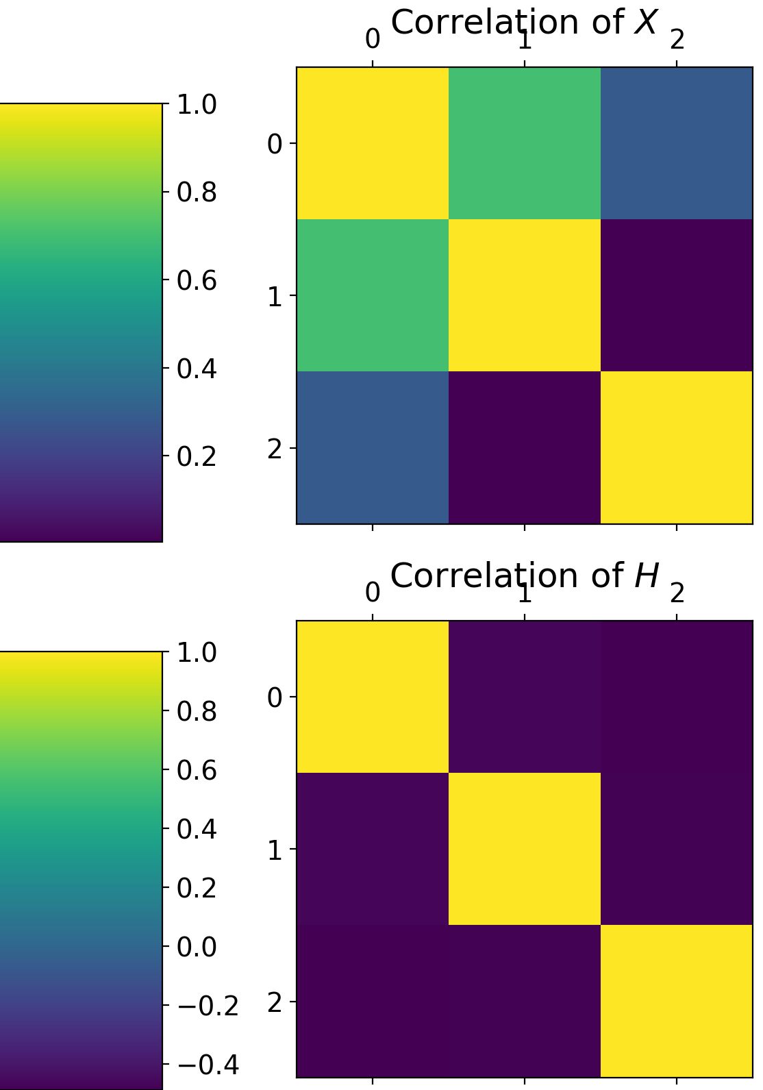
2. Simulated large-graph data. We also compare the GNN layers on a larger graph using the same 503-node chordal cycle graph as in Fig. 5, and simulate , where , is the -th Chebyshev polynomial, , being the adjacency matrix and the degree matrix, and . Fig. A.6 (ChebNet) and A.7 (L3Net) in appendix B.2 show that the iGNN model learns to generate samples close in distribution to the ground truth, as reflected in the resemblance of the correlation matrices. For this dataset, both spectral and spatial GNN layers have sufficient expressiveness to learn the data distribution.
7 Discussion
In this work, we developed the iGNN model, a conditional generative deep model based on invertible normalizing flow ResNet for inverse graph prediction problems. The model encodes the conditional distribution into a parametric distribution by a one-to-one mapping from to , which allows forward prediction and generation of input data given an outcome (including the construction of uncertainty sets for ). The scalability of the iGNN model to large graphs is achieved by taking a factorized formula of with a provable component separation guarantee, and the computational scalability is achieved via adopting GNN layers. In addition, the invertibility of the flow network is ensured by a Wasserstein-2 regularization, which can be computed efficiently in the forward pass of the flow network and is compatible with free-form neural network layer types in the residual blocks. Theoretically, we analyzed the existence of invertible flows and examined the expressiveness of GNN layers on graph data to express these normalizing flows. In experiments, we showed the improved performance of iGNN over alternatives on real data and the scalability of the iGNN model on large graphs.
There are several future directions to extend the work. On the theoretical side, first, under the framework of our problem, more analysis of the case will be useful to go beyond the current Assumption 1. Second, it would be interesting to develop a full approximation result on how the theoretical continuous-time flow identified in Section 4 can be approximated by a deep residual network. Specifically, one can construct a discrete-time flow on with time stamps to approximate the continuous-time one. for the Benamou-Brenier flow, and for the Fokker-Planck flow (so as to achieve -closeness to the normal density at time ). The smoothness of the velocity field in both cases, cf. Propositions 4.2 and 4.3, implies that at each time stamp , may be approximated by a shallow residual block with finite many trainable parameters based on universal approximation theory. Compositing the time steps constructs a neural network approximation of the flow with a provable approximate generation of the data density . The precise analysis is left to future work. At last, one may be curious about the connection between the encoding scheme of iGNN model and the Gaussian channel. If we view as the input of the channel and the output as given by , for noise , then the separation of components can be viewed as a requirement to ensure the error probability of the linear decoder to be sufficiently small. A natural question arises in how many components can be encoded in this way and subsequently decoded (classified) successfully, for instance, by considering a compact encoding domain. To further develop the methodology, one interesting question is to consider the regression problem, where the outcome takes continuous (rather than categorical) values. Another related question is the inverse of the graph classification problem, that is, given an output label of a whole graph, generate the input graph data including changing graph topology and node/edge features. The current work tackles the node classification setting, and some of our techniques may extend to the graph classification setting.
Acknowledgement
The work is supported by NSF DMS-2134037. C.X. and Y.X. are supported by an NSF CAREER Award CCF-1650913, NSF DMS-2134037, CMMI-2015787, DMS-1938106, and DMS-1830210. X.C. is partially supported by NSF, NIH and the Alfred P. Sloan Foundation.
References
- [1] Abdullah M. Al-Shaalan. Reliability evaluation of power systems. Reliability and Maintenance - An Overview of Cases, 2020.
- [2] Lynton Ardizzone, Jakob Kruse, Carsten Lüth, Niels Bracher, Carsten Rother, and Ullrich Köthe. Conditional invertible neural networks for diverse image-to-image translation. In DAGM German Conference on Pattern Recognition, pages 373–387. Springer, 2020.
- [3] Lynton Ardizzone, Jakob Kruse, Carsten Rother, and Ullrich Köthe. Analyzing inverse problems with invertible neural networks. In International Conference on Learning Representations, 2019.
- [4] Lynton Ardizzone, Carsten Lüth, Jakob Kruse, Carsten Rother, and Ullrich Köthe. Guided image generation with conditional invertible neural networks. arXiv preprint arXiv:1907.02392, 2019.
- [5] Jens Behrmann, Will Grathwohl, Ricky TQ Chen, David Duvenaud, and Jörn-Henrik Jacobsen. Invertible residual networks. In International Conference on Machine Learning, pages 573–582. PMLR, 2019.
- [6] Jean-David Benamou and Yann Brenier. A computational fluid mechanics solution to the monge-kantorovich mass transfer problem. Numerische Mathematik, 84(3):375–393, 2000.
- [7] Alex Beutel, Leman Akoglu, and Christos Faloutsos. Graph-based user behavior modeling: from prediction to fraud detection. In Proceedings of the 21th ACM SIGKDD international conference on knowledge discovery and data mining, pages 2309–2310, 2015.
- [8] François Bolley, Ivan Gentil, and Arnaud Guillin. Convergence to equilibrium in wasserstein distance for fokker–planck equations. Journal of Functional Analysis, 263(8):2430–2457, 2012.
- [9] Luis A Caffarelli. Boundary regularity of maps with convex potentials–ii. Annals of mathematics, 144(3):453–496, 1996.
- [10] Ricky TQ Chen, Jens Behrmann, David K Duvenaud, and Jörn-Henrik Jacobsen. Residual flows for invertible generative modeling. Advances in Neural Information Processing Systems, 32, 2019.
- [11] Xiuyuan Cheng, Zichen Miao, and Qiang Qiu. Graph convolution with low-rank learnable local filters. In International Conference on Learning Representations, 2021.
- [12] Djork-Arné Clevert, Thomas Unterthiner, and Sepp Hochreiter. Fast and accurate deep network learning by exponential linear units (elus). In International Conference on Learning Representations, 2016.
- [13] Michaël Defferrard, Xavier Bresson, and Pierre Vandergheynst. Convolutional neural networks on graphs with fast localized spectral filtering. Advances in neural information processing systems, 29, 2016.
- [14] Laurent Dinh, Jascha Sohl-Dickstein, and Samy Bengio. Density estimation using real NVP. In International Conference on Learning Representations, 2017.
- [15] Ian J. Goodfellow, Jean Pouget-Abadie, Mehdi Mirza, Bing Xu, David Warde-Farley, Sherjil Ozair, Aaron C. Courville, and Yoshua Bengio. Generative adversarial nets. In NIPS, 2014.
- [16] Henry Gouk, Eibe Frank, Bernhard Pfahringer, and Michael J Cree. Regularisation of neural networks by enforcing lipschitz continuity. Machine Learning, 110(2):393–416, 2021.
- [17] Will Grathwohl, Ricky T. Q. Chen, Jesse Bettencourt, and David Duvenaud. Scalable reversible generative models with free-form continuous dynamics. In International Conference on Learning Representations, 2019.
- [18] Arthur Gretton, Karsten M. Borgwardt, Malte J. Rasch, Bernhard Schölkopf, and Alex Smola. A kernel two-sample test. J. Mach. Learn. Res., 13:723–773, 2012.
- [19] Ishaan Gulrajani, Faruk Ahmed, Martín Arjovsky, Vincent Dumoulin, and Aaron C. Courville. Improved training of wasserstein gans. In NIPS, 2017.
- [20] Han Huang, Jiajia Yu, Jie Chen, and Rongjie Lai. Bridging mean-field games and normalizing flows with trajectory regularization. arXiv preprint arXiv:2206.14990, 2022.
- [21] Phillip Isola, Jun-Yan Zhu, Tinghui Zhou, and Alexei A. Efros. Image-to-image translation with conditional adversarial networks. 2017 IEEE Conference on Computer Vision and Pattern Recognition (CVPR), pages 5967–5976, 2017.
- [22] Richard Jordan, David Kinderlehrer, and Felix Otto. The variational formulation of the fokker–planck equation. SIAM journal on mathematical analysis, 29(1):1–17, 1998.
- [23] Herman Kahn. Use of different monte carlo sampling techniques. 1955.
- [24] Diederik P. Kingma and Jimmy Ba. Adam: A method for stochastic optimization. CoRR, abs/1412.6980, 2015.
- [25] Diederik P. Kingma and Max Welling. Auto-encoding variational bayes. CoRR, abs/1312.6114, 2014.
- [26] Diederik P. Kingma and Max Welling. An introduction to variational autoencoders. Foundations and Trends® in Machine Learning, 12(4):307–392, 2019.
- [27] Ivan Kobyzev, Simon JD Prince, and Marcus A Brubaker. Normalizing flows: An introduction and review of current methods. IEEE transactions on pattern analysis and machine intelligence, 43(11):3964–3979, 2020.
- [28] Christian Ledig, Lucas Theis, Ferenc Huszár, Jose Caballero, Andrew P. Aitken, Alykhan Tejani, Johannes Totz, Zehan Wang, and Wenzhe Shi. Photo-realistic single image super-resolution using a generative adversarial network. 2017 IEEE Conference on Computer Vision and Pattern Recognition (CVPR), pages 105–114, 2017.
- [29] Alexander Lubotzky. Discrete groups, expanding graphs and invariant measures. In Progress in mathematics, 1994.
- [30] James Lucas, G. Tucker, Roger B. Grosse, and Mohammad Norouzi. Understanding posterior collapse in generative latent variable models. In DGS@ICLR, 2019.
- [31] Alireza Makhzani, Jonathon Shlens, Navdeep Jaitly, and Ian J. Goodfellow. Adversarial autoencoders. ArXiv, abs/1511.05644, 2015.
- [32] Mehdi Mirza and Simon Osindero. Conditional generative adversarial nets. ArXiv, abs/1411.1784, 2014.
- [33] Derek Onken, S Wu Fung, Xingjian Li, and Lars Ruthotto. Ot-flow: Fast and accurate continuous normalizing flows via optimal transport. In Proceedings of the AAAI Conference on Artificial Intelligence, volume 35, 2021.
- [34] George Papamakarios, Eric T Nalisnick, Danilo Jimenez Rezende, Shakir Mohamed, and Balaji Lakshminarayanan. Normalizing flows for probabilistic modeling and inference. J. Mach. Learn. Res., 22(57):1–64, 2021.
- [35] Tim Salimans, Ian Goodfellow, Wojciech Zaremba, Vicki Cheung, Alec Radford, Xi Chen, and Xi Chen. Improved techniques for training gans. In D. Lee, M. Sugiyama, U. Luxburg, I. Guyon, and R. Garnett, editors, Advances in Neural Information Processing Systems, volume 29. Curran Associates, Inc., 2016.
- [36] Benjamín Sánchez-Lengeling and Alán Aspuru-Guzik. Inverse molecular design using machine learning: Generative models for matter engineering. Science, 361:360 – 365, 2018.
- [37] Thomas C Sideris. Ordinary differential equations and dynamical systems, volume 2. Springer, 2013.
- [38] Gábor J. Székely and Maria L. Rizzo. Energy statistics: A class of statistics based on distances. Journal of Statistical Planning and Inference, 143:1249–1272, 2013.
- [39] Asuka Takatsu. Wasserstein geometry of gaussian measures. Osaka Journal of Mathematics, 48(4):1005–1026, 2011.
- [40] MTCAJ Thomas and A Thomas Joy. Elements of information theory. Wiley-Interscience, 2006.
- [41] Cédric Villani. Optimal transport: old and new, volume 338. Springer, 2009.
- [42] Cédric Villani. Topics in optimal transportation, volume 58. American Mathematical Soc., 2021.
- [43] Antoine Wehenkel and Gilles Louppe. Unconstrained monotonic neural networks. Advances in neural information processing systems, 32, 2019.
- [44] Zonghan Wu, Shirui Pan, Fengwen Chen, Guodong Long, Chengqi Zhang, and S Yu Philip. A comprehensive survey on graph neural networks. IEEE transactions on neural networks and learning systems, 32(1):4–24, 2020.
- [45] Fang Yang, Kunjie Fan, Dandan Song, and Huakang Lin. Graph-based prediction of protein-protein interactions with attributed signed graph embedding. BMC bioinformatics, 21(1):1–16, 2020.
- [46] Mei Yu, Zhuo Zhang, Xuewei Li, Jian Yu, Jie Gao, Zhiqiang Liu, Bo You, Xiaoshan Zheng, and Ruiguo Yu. Superposition graph neural network for offshore wind power prediction. Future Generation Computer Systems, 113:145–157, 2020.
- [47] Jun-Yan Zhu, Taesung Park, Phillip Isola, and Alexei A. Efros. Unpaired image-to-image translation using cycle-consistent adversarial networks. 2017 IEEE International Conference on Computer Vision (ICCV), pages 2242–2251, 2017.
- [48] Bo Zong, Qi Song, Martin Renqiang Min, Wei Cheng, Cristian Lumezanu, Dae ki Cho, and Haifeng Chen. Deep autoencoding gaussian mixture model for unsupervised anomaly detection. In International Conference on Learning Representations, 2018.
Appendix A Proofs
A.1 Proofs in Section 3
Proof of Lemma 3.1.
For any , and , define , . Define
| (A.1) |
and we claim that
| (A.2) |
If true, then let
we have that
thus is an -support of for all . Meanwhile, for any , and , we know that and . By construction (A.1), we know that if we center the origin at and rotate the coordinates in such that is along the first coordinate, then , and . This gives that
Thus .
It remains to show (A.2) to finish the proof of the lemma. By construction, this is equivalent to show that for ,
where we have that due to that . Note that , thus
where the last equality is by the definition of . ∎
Proof of Proposition 3.2.
Let , then here equals in Lemma 3.1, where the dimension in Lemma 3.1 is here. Applying Lemma 3.1 to the -component Gaussian mixture distribution in , there exist sets such that , and
| (A.3) |
For each from the possible graph labels, define
| (A.4) |
which is an -way rectangle in . Due to the factorized form of as in (6), we know that
By the elementary relation that for , we have that
This shows that and thus is an -support of in .
A.2 Proofs in Section 4
Proof of Proposition 4.1.
By definition, for each ,
The minimization of (13) can be written as
| (A.5) |
and the minimization in (14) is with the extra constraint that . It suffices to show that the minimization over ’s only (by requiring and eliminating the variables ’s) achieves the same minimum of minimizing over both ’s and ’s in (A.5). Suppose (A.5) is minimized at ’s and ’s, and the minimum equals
| (A.6) |
where , and we also have for . This guarantees that
that is, if we replace with in (A.6) the value of the equation remains the same. This shows that the minimum of (A.5) can be achieved by the objective of (14) at a set of transport maps ’s. ∎
Proof of Proposition 4.2.
The Wasserstein-2 optimal transport , and because both and standard normal are smooth and have all finite moments in , is also smooth [9]. The optimal has the expression that
| (A.7) |
where is the displacement interpolation for [42]. Because both and are smooth, is smooth on . For any bounded domain , has finite -Lipschitz constant on , which suffices for the well-posedness of the IVP [37]. ∎
A.3 Proofs in Section 5
Proof of Lemma 5.1.
Proof of Lemma 5.2.
Proof of Lemma 5.3.
To prove (i), note that
| (A.11) |
Because is the midpoint of the interval where lies on, we have that for all ,
| (A.12) |
where in the last inequality we have use that . We now truncate to the expansion (A.11) up to , and define
the polynomial is a polynomial of degree for and reduces to when . By (A.12) and that the number because , we have that for all ,
which holds uniformly for all .
To prove (ii), use the expansion of as
| (A.13) |
and define as the truncated summation up to , which is a polynomial of degree . Similarly, we can bound the residual as
| (A.14) |
where we use that and ,
| (A.15) |
The bound (A.14) holds uniformly for all and . ∎
Proof of Theorem 5.4.
Under the assumption of the theorem, Lemma 5.3 applies with .
Proof of (i): We set , which is a polynomial of degree at most since the degree of is at most . Recall that satisfies (C1)(C2), and by (26),
We bound and respectively.
By definition of as in (23), for any invertible real symmetric matrix , denote , ,
By that , one can verify that
and thus
By (C2), ; By (21), , and then
Meanwhile, by (C1), and then similarly, . Putting together,
| (A.16) |
where the last inequality is by that .
To bound , we introduce the following lemma which can be verified directly by definition (in below).
Lemma A.1.
Let be a real symmetric matrix and . For real-valued functions and on ,
By definition of and that by (C1),
| (A.17) |
where and . Because , by the elementary inequality , we have
| (A.18) |
by that . Back to (A.17), we have
| (A.19) |
Putting together (A.16) and (A.19) proves (27) by triangle inequality for all .
Proof of (ii): We set , which is a polynomial of degree at most . Recall that satisfies (C1)(C2), and then
To bound , by definition of as in (23), the constants and as before, we have
and then
By that , and also with that for ,
and same with . Together with By (C2), we have
| (A.20) |
where we have used that when .
Proof of Lemma A.1.
Suppose is -by-. Let be the eigen-decomposition, where is an orthogonal matrix consisting of columns , , and are the diagonal entries of (the associated eigenvalues). Then
and thus
due to that all lie inside . ∎
Appendix B Additional experimental details
B.1 Experimental set-up
B.1.1 Computation of
To compute the log determinant in (4), we adopt the following unbiased log determinant approximation technique as proposed in [10]. Let denote the output from a generic ResNet block with parameter . First, observe that for any input , because the matrix is non-singular. We thus have . As a result, the trace of the matrix logarithm can be expressed as
| (A.22) |
Based on (A.22), which takes infinite time to compute, we can obtain an unbiased estimator in finite time based on the “Russian roulette“ estimator approach [23, 10]. For a ResNet as a concatenation of ResNet blocks, the approximation is applied to each block and summed over all blocks. Lastly, to speed up gradient computation of the approximation, we further adopt memory efficient backpropagation through the early computation of gradients [10].
B.1.2 Model evaluation metrics

MMD statistics metric. Given two sets of samples of same sample size , the MMD two-sample statistic between and is defined as
| (A.23) |
where we use the radial basis kernel with .
For the -class conditional distribution , where we denote by the set of samples , the overall MMD statistic is defined using (A.23) as
| (A.24) |
Note that on graph data where concatenates all nodal labels, the summation is over all types of (up to many).


Energy statistic metric. Given two sets of samples , The energy statistic under norm is defined as
| (A.25) |
For -class conditional distribution , the weighted energy statistics is defined using (A.25) as
| (A.26) |
Computation of the weighted statistics on graph data is identical to that of the weighted MMD statistics on graph.
Model invertibility error. We see from Fig. A.2 that iGNN under the Wasserstein-2 regularization ensures model invertibility up to very high accuracy.


B.1.3 Construction of simulated graph data
We first describe the construction of simulated graph data on small graphs (corresponding to Figures A.4 and 9). Each node has a binary label so that is a binary vector. Conditioning on a specific binary vector out of the eight choices, the distribution of is defined as
where is the graph averaging matrix. The distribution of is specified as:
- •
In Figure 9, we let
(A.27) - •
On large graphs (corresponding to Fig. 5), each node has a binary label so that is a binary vector. Conditioning on a specific binary vector out of the eight choices, the distribution of is defined as
where denotes a counter-clockwise rotation matrix for 90 degrees (applied node-wise to each two-dimensional nodal feature) and is the graph averaging matrix, where is the degree matrix. We choose so that a soft graph averaging is applied to the hidden variables .
B.2 Additional experimental results
This subsection contains experimental results to augment those in the main text. In particular,
- •
- •
- •
- •


B.3 Hyperparameter selection
We first summarize the hyperparameters used in our experiments and then verify that iGNN is insensitive to alternative hyperparameter choices.
- •
Mixture distribution in with 8 components (cf. Fig. 4): we let iGNN contain 40 ResNet blocks, each of which is built with fully-connected layers with two hidden layers. We fix the learning rate at 5e-4 and train with a batch size of 1000. We fix the regularization factor of the loss as 1.
- •
- •
Conditional generation on large graph (cf. Fig. 5): we let iGNN contain 5 ResNet blocks, where the first hidden layer of each block is an L3Net layer. We fix the learning rate at 1e-3 and train with a batch size of 100. We fix the regularization factor of the loss as 0.375/503.
- •
Solar ramping event (cf. Fig. 6): we let iGNN contain 40 ResNet blocks, where the first hidden layer of each block is a Chebnet layer. We fix the learning rate at 1e-4 and train with a batch size of 150. We fix the regularization factor of the loss as 0.375/503.
- •
Traffic anomaly detection (cf. Fig. 8): we let iGNN contain 40 ResNet blocks, where the first hidden layer of each block is an L3Net layer. We fix the learning rate at 1e-4 and train with a batch size of 200. We fix the regularization factor of the loss as 1.
- •


Insensitivity of iGNN to for regularization. We verify that as long as the ResNet is invertible under the choice of , the value of only affects the training efficiency but not the final generative quality. This is because larger values restrict more the amount of movement by the ResNet, which thus potentially takes longer training epochs before transporting the distribution to at each . Fig. A.8 shows iGNN performance on conditional generation of data on large graph, where we increase the factor by 503 times. The performance is nearly identical to that in Fig. 5. On the other hand, Fig. A.9 visualizes the generative loss of iGNN on unconditional generation of data on large graph, where we increase the factor by 5 times. Comparing to the generative loss in Fig. A.6, the loss takes more epochs to converge, but eventual generative performance are nearly identical.
Insensitivity of iGNN to other hyperparameters. We verify that iGNN is insensitive to other hyperparameter choices such as learning rate, batch size, and the number of residual blocks. Figures A.9 shows the loss trajectories of iGNN under alternative choices of these hyperparameters, where the setup is identical to that in Fig. A.6. We see that training losses under these choices all converge reasonably fast. We omit comparing the covariance matrices because the generative quality barely differs from those in Fig. A.6.


