On the structure of pointsets with many collinear triples
Abstract
It is conjectured that if a finite set of points in the plane contains many collinear triples, then part of the set has a structure. We will show that under some combinatorial conditions, such pointsets have special configurations of triples, proving a case of Elekes’ conjecture. Using the techniques applied in the proof, we show a density version of Jamison’s theorem. If the number of distinct directions between many pairs of points of a point set in a convex position is small, then many points are on a conic.
1 Introduction
In this paper, we investigate planar pointsets spanning many collinear triples. If three -element pointsets are well separated (mutually avoiding) and there are collinear triples, one point from each, it contains a Pappus configuration. Elekes conjectured it for general pointsets containing many collinear triples. We prove a special case in Theorem 5. If one of the three separated pointsets consists of collinear points, then a strong structural result is proved in Lemma 19: a positive fraction of the remaining points are on a conic. As a corollary, we prove another conjecture of Elekes in Theorem 15. If the number of distinct directions between many pairs of points of a point set in a convex position is small, then many points are on a conic.
It is a classical and essential problem in discrete geometry to understand the structure of finite planar pointsets defining many lines containing at least three points of this set of points. An excellent survey article on many related problems is written by Borwein and Moser [5], and several open problems are mentioned in the problem book of Brass, Moser, and Pach (Chapter 7 in [6]). Solving a famous conjecture of Dirac and Motzkin, the following statement was proved by Green and Tao in 2013 [20].
Theorem 1
Suppose that is a set of points in the plane. Then there are at most lines that contain at least three points of provided is large enough.
For a given set of points, a line is determined by if it contains at least two points of If such a line has exactly two points, it is called an ordinary line. Green and Tao proved a strong structure theorem which states that if has at most ordinary lines, then all but points of lie on a cubic curve if is sufficiently large depending on (in this result is a constant or a very slowly growing function of ). Unfortunately, almost nothing is known about the structure of when there are lines with at least three points of where Elekes conjectured that here, under this weaker condition, ten or more points of lie on a (possibly degenerate) cubic, provided that (see, e.g. Conjecture 2.1 in [15]). There are some structural results for -element pointsets with collinear triples, like in [34] and [11], but these are not enough to prove Elekes’ conjecture on “ten points on a cubic”. There is another related conjecture (problem) of Elekes (see in [44] and in [32]), which was the main inspiration for this work.
Problem 2 (Elekes [44])
For fixed suppose that the edges of a graph with vertices and edges are well-coloured using colours (i.e., no two edges of the same colour are incident upon a common vertex). If is sufficiently large, must contain a six-cycle with opposite edges having the same colour?
Elekes gave another formulation of the problem in [44]. If the colours of the edges are represented by extra vertices, each added to the edges with its colour, then we can state the problem (now stated as a conjecture) in terms of 3-uniform hypergraphs. A 3-uniform hypergraph is linear if any two edges have at most one vertex common. In a 3-uniform hypergraph, six edges are called a tic-tac-toe if they intersect each other like the rows and columns of a tic-tac-toe board.
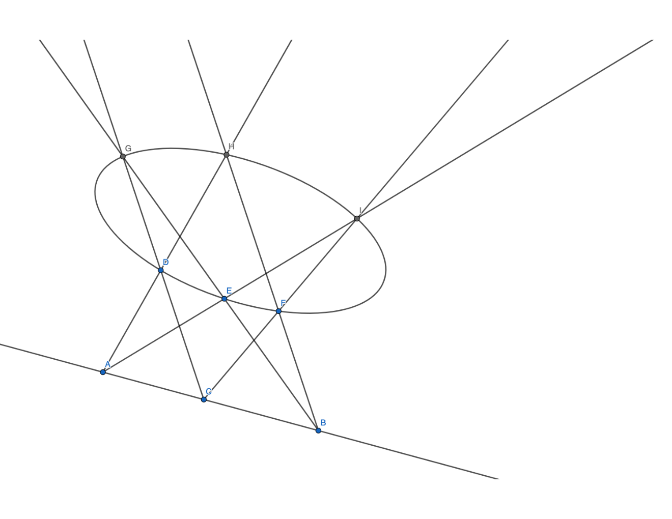
It follows from the converse to Pascal’s theorem, called Braikenridge–Maclaurin theorem [26] that in a tic-tac-toe configuration of collinear triples in the plane if three pairwise independent11 1 Two vertices are independent if there is no edge containing both. points are collinear, then the remaining six points are on a conic (Figure 2). A 3-uniform linear hypergraph on vertices has at most edges. Elekes conjectured that if it contains no tic-tac-toe, then it should be sparse.
Conjecture 3
If a 3-uniform linear hypergraph on vertices contains no tic-tac-toe, it is sparse; it has edges. (For any there is an such that if then the number of edges is at most )
This conjecture was refuted by Gishboliner and Shapira, giving a nice construction for 3-uniform hypergraphs on vertices with edges without tic-tac-toe [19]. Earlier, Füredi and Ruszinkó even conjectured that there are 3-uniform hypergraphs on vertices with edges (almost Steiner triple systems) without a tic-tac-toe [17]. This conjecture is still open.
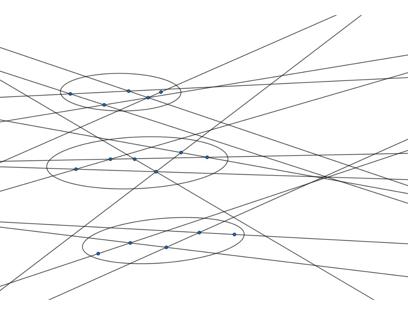
In this paper, we will prove Conjecture 3 when the edges are collinear triples in some pointsets. We show that if the edges of a 3-uniform hypergraph are defined by collinear triples from three sets of points, there are vertices spanning many edges. In the last section, we prove that if one of the three sets consists of collinear points under some combinatorial conditions, then a large fraction of the other two sets are on a conic. As noted in [13] (see the quote after Conjecture 14 below), without extra conditions, this statement would not hold. For example, taking a projective image of an integer square grid with the line of infinity, there are collinear triples with two points in the grid and one on the line at infinity (the points of the directions), while the grid contains at most points of a parabola and points of other conics22 2 This claim can be recovered from multiple sources, see, e.g. Lemma 5. in [23]. (Figure 3).

In Section 4.2 of the paper, we prove a strong structural result for some pointsets where many pairs determine few distinct directions. Using the combinatorial model for analyzing sets with few directions due to Eli Goodman and Ricky Pollack [21], Jamison proved the following structural result.
Theorem 4 (Jamison [22])
If an -element pointset contains no three collinear points and determines directions, then it is affinely equivalent to the vertices of a regular -gon, i.e. the points are on a conic.
The Goodman-Pollack method is nicely explained in Chapter 12 of the Proofs from the BOOK by Aigner and Ziegler [1] where they proved Ungar’s theorem [41] on the minimum number of distinct directions determined by non-collinear points in the plane.
In the problem of characterizing pointsets determining few directions, we show that if two -element sets, and , contain distinct pairs determining at most directions, then – under some combinatorial assumptions – a positive fraction of the points of is on a conic.
2 Elekes’ conjecture for collinear triples
While Conjecture 3 was disproved in general, we show that it holds for certain sets of collinear triples. Given three pointsets in the plane, and we say that the three sets are mutually avoiding sets if no line determined by two points in a set intersects the two convex hulls of the other two pointsets. The concept of mutually avoiding sets is often used in discrete and computational geometry, like in [2], [42], [27] and [29]. It was proved in [2] that any planar -element pointset in general position contains two mutually avoiding subsets of size at least
Theorem 5
For any constant, there is a threshold , so the following holds. Let be mutually avoiding -element pointsets in the plane. Let us suppose that there are at least collinear triples, where and If then there is a tic-tac-toe configuration among the collinear triples.
We will show a density version of Theorem 5: If we select a subset of the collinear triples spanned by and of size at least then in this subset, there will be a tic-tac-toe configuration. In this paper’s proofs, when we refer to collinear triples (or simply triples or edges), these are triples in our selected subset of the geometrically collinear triples. We can remove them in the proofs, even if the three points remain collinear triple in the geometric sense. In the proof of Theorem 5, we are going to use the geometric properties of the triples and the theorem of Ruzsa and Szemerédi twice (Theorem 6 below). Because of the use of the Ruzsa-Szemerédi theorem, our bound on is rather weak.
As was mentioned earlier, it follows from the Brackenridge–Maclaurin theorem that if in Theorem 5 set is a set of collinear points, then three points in and three in are lying on the same conic (Figure 2). We will analyze this case in Section 4 of the paper.
2.1 Proof of Theorem 5
During the proof, we will assume that set is the set of the middle points of the collinear triples. Since the three sets and are mutually avoiding, any point in sees every point in in the same clockwise order and sees every point in in the same anticlockwise order in which we are using to label the points as Now we sweep a line through an arbitrary point of anticlockwise to label With this labelling, the following conditions hold:
- •
If and are collinear triples and then
- •
If and are collinear triples and then
- •
If and are collinear triples and then
This ordering will be crucial in the proof since we will search for configurations (the second graph, labelled by b, in figure 5) where the vertices in the same set are close to each other. We will see that in this ordered geometric setting, collinear triples determine some configurations on not too many, close point-pairs ( and are constants depending on only). Then we can apply the Ruzsa-Szemerédi theorem again to find a configuration, with nine edges spanned by twelve edges. This configuration contains tic-tac-toe (Figure 5).

2.1.1 Finding many skinny (6,3) configurations
We begin this subsection by stating the theorem of Ruzsa and Szemerédi.
Theorem 6 (Ruzsa-Szemerédi [33])
For any , there is a threshold, such that if a 3-uniform hypergraph has vertices and at least edges, then there are six vertices spanning at least three edges of the hypergraph.
In our application, the hypergraph is a linear three-partite 3-uniform hypergraph since the edges a defined by collinear triples with one vertex in each set. The only configuration which is possible is isomorphic to the second figure (b,) in Figure 5.
Definition 7
A configuration in the sets is called -skinny if the spanning vertices are and
Lemma 8
For any there is a and natural number such that collinear triples () determine at least -skinny configurations provided is large enough. Moreover, one can assume that the configurations are edge-disjoint; they don’t share collinear triples.
P r o o f. Let us choose a large constant We will determine the value of during the proof. It is a constant, so for the sake of simplicity, we can assume that divides Let us partition the vertices of and into classes such that each partition class contains consecutive elements. etc. and etc.
Definition 9
For an pair, is said to be -good if there are at least collinear triples where and By saying that an triple is -good we mean that is -good for the pair, where and
Let us count the number of triples where is -good for .
For every let us complete the following pruning process:
- 1.
If the vertices of a contribute to less than triples with and any then let’s remove these triples (). Then we repeat the process with -s, if there are less than vertices in a forming a collinear triple with and some vertices of then remove the triples. Next, we check -s again, removing triples if there is less than triples with the vertices in this partition class. Then we check -s again and repeat this alternating process as long as possible. The total number of removed triples is denoted by . It is less than .
- 2.
Let us call triples and with point to be weak if the total number of collinear triples and is less than or, equivalently, is not -good for Remove all weak triples.
We have to show that after the second step, we still have many triples if there were many triples through . At this point, we have to use the geometric properties of sets and If there is a collinear triple and with point , then we can’t conclude that there are many triples between and through even in this geometric setting (see Figure 6).

On the other hand, a collinear triple guarantees that there are many triples either between and or in their neighbourhood. If there is a collinear triple between and via then let () denote the set of points in where there is another point in forming a triple with Similarly, () denote the set of points in where there is another point in forming a triple with Because of the first step, we know that both and are at least
For any triple, at least triples where and are triples between and 33 3 Let us suppose that When then at least triples are between and On the other side, for the triple at least triples , where and , are triples between and When then at least triples are between and
If is weak then both and should be among the first points or both are among the last points of and More precisely
After the first step of the pruning process, let’s check the triples starting with the least index in increasing order. By the previous observations, the longest sequence of weak triples is less than always followed by at least many -good triples (if there are triples left). If the number of triples through after the first step is denoted by , then the number of weak triples is at most
After the pruning process is finished for all the total number of removed triples is not more than
| (1) |
Since and , we have the following upper bound on the number of removed triples:
| (2) |
We still have about the quarter of the original triples, and now every triple is -good for the relevant pair. For reference in later applications, we record our partial result in the following claim.
Claim 10
For any there is a constant such that under the conditions of Theorem 5 at least triples are -good.
In the calculations leading to Claim 10, the parameter was set to be a constant, however, the bounds hold (with a larger error term) if is a slow-growing function of .
Note that up to this point, the only property we used for the pointset is that no line determined by the points of or by the points of intersects the convex hull of so Claim 10 holds under the weaker conditions that and are mutually avoiding and , and are avoiding
In the remaining part of the proof of Theorem 5, we ignore the linear error term, it does not affect the arguments. As the last pruning step, we check the number of the remaining collinear triples between the pairs for all If the number of triples is less than then remove all triples between and After this, we have left with at least triples, and whenever there is a triple between two partition classes and it is -good for and there are at least triples between and
We can apply the Ruzsa-Szemerédi theorem for triple systems between all pairs where we have at least one triple left between them. As we noted before, there are at least triples between them, and the number of points from forming the triples is at most
By Theorem 6, we can set large enough such that if the number of triples is at least on vertices, then it contains a configuration. It is satisfied if we choose We continue to work with this parameter The number of triples is at least , so there are at least distinct pairs so that there is a configurations spanned by the triples between and For every we select two points from and two points from such that the selected pairs span many configurations (together with the points of ) Let’s choose the pairs independently at random. The probability that both pairs of points of a configuration from and have been selected is So, there is a way to select points, two from every partition class of and such that the pairs which were chosen span at least distinct configurations. If the spanning vertices of such a configuration are denoted by then
What is left in the proof of Lemma 8 is to show that there is a constant such that many of the selected configurations satisfy For this, we are going to use the ordering (labelling) of In a configuration, there is one point in which is in two collinear triples, and the other in one triple. In at least half of the configurations, the order of the two types of points is the same. Let us suppose that the doubhas the smaller subscript in most of the earlier selected triples and keep these configurations only. We have at least configurations left. Every configuration has its pair of points in in one of the pairs selected in the random process. If the number of configurations on a selected pair is less than half the average when it is less than then throw them away. We have at least configurations left. Note that in any two configurations with the same pair of points in where the vertices are denoted by and the intervals and are disjoint, since the pairs, and are in different partition classes. (Figure 7 ).

Since these intervals of indices are disjoint, no pair in can hold more than configurations where the two points are far, when This proves the lemma with parameters and where
2.1.2 Using Ruzsa-Szemerédi again
To complete the proof of Theorem 5, we define a 3-uniform hypergraph, where the edges are the skinny configurations we are left with after the last step in the previous section. From the pointsets, and , the vertices of the new hypergraph are the pairs we selected in the random process. In pointset , let’s consider all pairs where For each such pair, we can assign an integer, the number of configurations containing this pair of points. We follow a greedy algorithm to select vertex disjoint pairs contributing to many skinny configurations.
- 1.
Select a pair with the highest assigned value, say .
- 2.
Remove all pairs where the or There are less than such pairs, and all removed pairs had a value less than
- 3.
If there are pairs left, go back to step one.
3 The Brown-Erdős-Sós conjecture for collinear triples
One of the most famous open problems in extremal combinatorics is the following:
Conjecture 11 (Brown-Erdős-Sós [7])
Fix . For every , there exists a threshold such that if is a 3-uniform hypergraph on vertices with , edges there exists a subset of vertices of which spans at least edges. (i.e. the hypergraph contains an configuration)
About 50 years later, the only known case of Conjecture 11 is when Theorem 6 above. We refer to [37] and [9] for some estimates and reviews of related works. Conjecture 11 has resisted all proof attempts in its general form. However, some special cases exist when even stronger statements can be proved. When the edges of the hypergraph are defined by a finite group with edges of the form , the underlying structure helps to find vertices spanning many edges. There are recent works proving such results like in [35],[38],[25],[43], and [28].
We proved the existence of configurations in large dense systems of collinear triples between three mutually avoiding pointsets. Removing points from this arrangement we have configurations, matching the numbers of the B-E-S conjecture. For larger values, we can get denser configurations, similar to the case of triples from finite groups. One way to prove such results is to iterate the method we used in the proof of Theorem 5. We can find many skinny configurations and consider them as edges of a 3-uniform graph on some four-tuples of points as vertices, and then apply Ruzsa-Szemerédi again. This way we would get edges on vertices, a configuration. One would get configurations by further iterations. But this method involves the iteration of the Ruzsa-Szemerédi theorem, which gives a very poor bound. On the other hand, we can use some elements of the previous proof to get better bounds than what would follow from the B-E-S conjecture, even in sparse systems.
Definition 12
A -complete collinear triple arrangement (or -system in short) consists of disjoint -element pointsets in denoted by and disjoint -element pointsets in denoted by such that for every there is a point such that for every the points and form a collinear triple.

A -system has at most points (some points might be the same) and edges.
Theorem 13
For any there are positive constants and a threshold such that the following holds. Let and be mutually avoiding -element pointsets in the plane such that no line determined by or determined by intersects the convex hull of the -element pointset . Let us suppose that there are at least collinear triples, where and If then there is a -system among the collinear triples.
P r o o f. We will use the calculations and notations leading to Claim 10 in the proof of Theorem 5. There are at least triples that are -good among triples. Set and . We will specify the value of later. If it is small enough, we can still assume that divides so the calculations before Claim 10 can be repeated with a non-constant . (If the number of triples in the arrangement was then we can throw away a few points and less than triples adjacent to them before starting the proof) With this setup and at least triples are -good since
We now estimate the number of -branches, the building blocks of -systems. The -branches are spanned by the partition classes for some They are formed by triples, sharing the same where and There are at least such branches. Let’s choose points from each and independently at random. If the number of -branches between and is denoted by then the probability of selecting the points of a -branch in and is so there is a selection of -tuples where the number of -branches is at least
| (3) |
Let us define an auxiliary bipartite graph where the vertices are the selected -tuples of points, and there is an edge between two if there was a -branch selected on the points. This graph has vertices in each vertex class and at least edges. By the Kővári-Sós-Turán theorem [24] if
then the graph contains a complete bipartite graph which proves the existence of a -system among the triples.
With the same exponent, by increasing the constant multiplier, a larger bipartite graph, will appear in the bipartite graph. Using a larger , one can guarantee a -system where all vertices are distinct, so the system contains exactly points. It is a particular configuration, which is an unavoidable collinear triple configuration, even in sparse systems.
4 When one set of points is collinear
In this section, we assume that set consists of collinear points, the convex hulls of and are not intersected by the line of , and no line determined by the points of intersects the convex hull of . Let us suppose that that there are collinear triples, where and In the case when is also a set of collinear points, Elekes proved that a positive fraction of the points of should also be collinear [12]. Elekes and Szabó proved the stronger statement that if the points of are on a conic, then a positive fraction of the points of is collinear (Theorem 5.2 in [15]). Our main result in this section is to show that if is collinear, then—under some additional conditions—many points of and are on a conic. Let’s recall another conjecture of Elekes, similar to the earlier ones:
Conjecture 14 (Elekes [14])
For every there is an with the following property. If and the number of directions determined by is at most then contains six points of a (possibly degenerate) conic. (As usual, a pair of lines is considered a degenerate conic.)
In his classical paper Sums vs Products [13] Elekes writes the following about his conjecture:
“It is very likely that Conjecture 14 holds for any number in place of six, for large enough. It was pointed out by M. Simonovits that one cannot expect conconic points in general (as shown by a square lattice.) However, some such points may exist for a suitable . Perhaps even can be found, provided that is the vertex set of a convex polygon.”
We will show a stronger, density version of this later statement.
Theorem 15
For any and , there is a constant, and a threshold , so the following holds. Let be a set of points in the plane in convex position (the vertex set of a convex polygon) such that at least point pairs determine at most distinct directions. If , then at least points of are on a conic.
Theorem 15 is a direct corollary of Lemma 19 below. Before proving Elekes’ conjecture, we recall a definition from projective geometry.
Definition 16
Two triangles are said to be perspectives from a line if the three points of intersections of corresponding sides all lie on a common line.
For some restricted arrangements of points in a convex position, we use the following standard definition
Definition 17
A set of points is a -cap relative to a line if the points are in convex position and the convex hull of the points and their orthogonal projections onto contains all points on the boundary.
The points of a -cap have a natural ordering based on the order of their projections onto . Using the ordering of the projection points from left to right (say), we write to indicate the ordering of the points .

Claim 18
Let be a -cap relative to a line . Then the two triangles spanned by and are not perspective from .
P r o o f. Consider four points forming a -cap relative to . Denote them as . The intersection point of the two lines containing and is denoted by . Let us suppose and let denote the projection of onto . We consider two cases
- •
. In this case, is not on the boundary of the convex hull of the points
which contradicts the assumption that the four points formed a -cap relative to . - •
. In this case, is not on the boundary of the convex hull of the points
which is a contradiction as in the previous case.
In the first section, we proved Theorem 5, which implies that if is a set of collinear points, then many 6-tuples of points from are on a conic. Now we have all the tools to show that a positive fraction of the points in is on a conic under some additional conditions.
Lemma 19
For any constant there is a threshold and so the following holds. Let be -element pointsets in the plane. Assume that and
- 1.
is a set of collinear points,
- 2.
the convex hulls of and are not intersected by the line of
- 3.
- 4.
no three points are collinear in ,
- 5.
and no two triples, and are perspective from the line of if
- 6.
there are at least collinear triples, where is between and where
Then at least points of are on a conic.
Before the proof, we give an example to show that something like conditions 4 and 5 is necessary for the conclusion. The example consists of two copies of a projection of the -dimensional integer grid where and the line at infinity, is the points of directions. Take a generic projection of onto the plane, and denote its points by . Choose a translation of denoted by such that and are mutually avoiding pointsets. We can select many point pairs, one from and one from , such that these pairs determine a few distances only. Define a set as points with all coordinates being far from the extremes. A point, is in iff for every With these parameters, we have
The points of the image of in and are denoted by and Any direction determined by two points and appears with multiplicity at least between points of and Select these directions (points) for set For the size of the following rough bound holds:
For a fixed constant, all conditions of Lemma 19 hold except conditions 4 and 5, and there is no conic containing more than points from In this construction, there are many similar triangle pairs and collinear triples.
4.1 The proof of Lemma 19
In the proof, we refer to the calculations preceding Claim 10. Based on the collinear triples, we will define a bipartite graph formed by 3-branches in a similar way as we did in the proof of Theorem 13. This bipartite graph is dense, so we will find a subgraph where contains two vertices (quadruples) and contains vertices. We will show then that the points of the corresponding points are on a low-degree algebraic curve. We will follow the exponents of during the calculations in case one is interested in conclusions similar to Lemma 19 when for some
4.1.1 The auxiliary bipartite graph
We will use the same parameters we had in the previous sections. By Claim 10 at least
| (4) |
triples are -good for the relevant pairs. We choose the parameter to be the least integer such that so if there is a triple between a pair after the pruning process before Claim 10, then there is at least one 3-branch between and We choose independently at random a triple of points in each and (). Since a constant nicely depending on , we can ignore the linear term in (4) which is at most about . There are at least distinct (but not necessarily vertex disjoint) 3-branches. The expected number of selected 3-branches - when both the top and bottom triples were selected - is at least
| (5) |
with a universal constant Now we are ready to define the auxiliary bipartite graph, . The vertices are the selected triples in -s and -s. There are such triples, so both vertex classes of the bipartite graph have size about denoted by Two vertices, given by and , are connected by an edge if the selected triples span a 3-branch.
There is a choice of triples such that the number of edges in is at least the expected number of edges in the random selection, it is at least If is large enough then there are two vertices in with at least common neighbours in Indeed, the number of 3-paths with the middle vertex in is
There is a pair, , out of the vertex-pairs wich are the end-vertices of at least different 3-paths. The two vertices, and have at least common neighbours.
Let us denote the two triples of points corresponding to and in by
and Since we selected one triple from the sets,
we can assume that
The corresponding triples in are denoted by where
4.1.2 Finding the algebraic curve in
To simplify the remaining calculations, let us apply a projective transformation, denoted by , which sends the first three points, to the pre-set coordinates , and the image of line is the -axis. A projective transformation could change convexity and other geometric relations among the points, but it preserves collinearity, and this is the only property we are using below.
 |
 |

We denote the image of by
and
For a point where the lines through and the points will intersect the axis in coordinates and (Figure 11). If is in as a midpoint of a 3-branch connecting to for some then there is also a 3-branch between and Since the three lines of this 3-branch
- 1.
- 2.
- 3.
are concurrent, we have the following identity for many
We want to show that the solutions, the zero set of the polynomial below, in equation (6) – the two-variable polynomial given by the determinant – is a one-dimensional algebraic set, it is an algebraic curve.
| (6) |
Even from the geometric way, we defined the equations, we see that the line is part of the zero set, but we will show that if then for any given value, has at most two possible values. For a fixed equation (6) is a quadratic equation in If it takes three or more different values then all three coefficients of the quadratic equation should be zero. The constant term is
which is zero only if The two points, and are on a line through the origin, i.e. there is a such that
The coefficient of the quadratic term is
which is zero only if
If we just want to see the proof of Theorem 15, then at this point we are done, since our selection of the two triples of points from the convex point set doesn’t allow such accidents. For the proof of Lemma 19 let’s complete the calculations of coefficients. We will see that there are pairs of triples where the zero set of the polynomial in (6) is a two-dimensional set.
The coefficient of the linear term is a bit harder to calculate; it is
Assuming that the other two coefficients are zero, i.e. and this coefficient is
which is zero only if
If the coordinates of the three points satisfy the equations
| (7) |
then, and only then, the zero set of the polynomial in (6) is a two-dimensional set. See for example Figure 12, where we set the three points as and

If all three conditions of (7) are satisfied then and are perspective from the -axis. Two common intersection points on the -axis are easy to find from the first two conditions; these are and . The line of and intersects at the point The equation of the line through is
After substituting the values from (7), one can check that this line intersects the axis at as well. For completeness, we include a simple calculation. Setting and using the identities in (7) we have
By the assumptions of Lemma 19, does not contain two triples perspective from so the equation in (6) defines an algebraic curve. After factoring out the line we were left with a degree two polynomial in two variables
which defines a (possibly degenerate) conic, so at least points of are on a conic.
4.2 Few directions in a convex point set
Let’s prove Theorem 15 first, and then we prove a stronger statement.
P r o o f. [of Theorem 15]: The convex point set can be separated into two sets and by a line such that out of the point pairs at least have one point in and the other one in Let’s apply a projective transformation which moves the line of infinity to the real plane, to a line parallel to which keeps the points of in convex position on the same halfplane determined by . The set is defined by the points of directions of the point pairs in one point in and the other is in From the conditions of the theorem, we have If, say, is closer to then applying Lemma 19 with and shows that at least points of are on a conic, where depends on only.
After choosing the separating line we can select the projective transformation such that either or are the pointsets closer to Because of that, we know that both and contain many points from conics. However, we don’t know whether the two conics are the same or not. The following theorem, one of our main results, addresses this question.
Theorem 20
For any and there is a constant, and a threshold so the following holds. Let be a set of points in the plane in convex position, and is a set of point pairs, which determine at most distinct directions. If and , then there is an such that and the points of are on a conic.
P r o o f. We follow the previous proof first with the additional step: before applying Lemma 19, we remove points from (let’s assume that is closer to ) which contribute in few directions with in . The set is defined as By the previous calculations We can consider as the edge set of the bipartite graph Let’s remove the vertices from which have degree less than This reduced set is denoted by and We apply Lemma 19 with parameters and as the points of directions on (also denoted by ). Now we have a set which is large, its points are on a conic, and
for some constants depending on and only. We keep the points of and and move back to the infinity and back on the ”other side“ so now is closer to Let’s apply Lemma 19 again, now with and is the set of direction points on the new It follows that there is a such that there is a set of points, which is on a conic, and Now we have two conics and a line containing many collinear triples. This answers Elekes’ related question, cited after Conjecture 14 already, but we can go a bit further using a result of Elekes and Szabó.
We use the following theorem to show that and are the same conics, which completes our proof.
Theorem 21 (Elekes-Szabó [15])
For every and positive integer there exist and with the following property. Let be (not necessarily distinct) irreducible algebraic curves of degree at most in the plane Assume that and
- 1.
no two are identical straight lines;
- 2.
with ;
- 3.
The number of collinear triples with is at least
Then is a cubic.
In the theorem, it is required that the three curves, in our case and are irreducible. We can suppose that because if or contains a linear component, then by the result of Elekes we mentioned earlier in the introduction of this section, we had three lines with some collinear triples proving Theorem 20 (Elekes’ result is in [12]).
5 Open problems
Many of the related conjectures of Erdős and Elekes remain open. Here we list a few questions where the tools we used in this paper might be useful.
- 1.
- 2.
- 3.
Scott’s problem on the minimum number of directions was solved in 3-space by Pach, Pinchasi, and Sharir in [30]. What structural results can one guarantee if the number of directions determined by two sets in space is very small?
- 4.
Let us suppose that four mutually avoiding -elements pointsets and have collinear four-tuples where and Can we conclude that then at least 5 points are collinear in ? (or in any other set). This problem is closely related to a question of Erdős [16]; is it true that if points contain collinear 4-tuples, then it should contain five collinear points? For some lower bounds and related results, see [36].
- 5.
Are there better bounds for the Brown-Erdős-Sós conjecture for collinear triples than what we had in Theorem 13? Maybe – similar to the case with triples from finite groups – there is a constant, such that the following holds. For any and , there is a threshold, such that if and there are at least collinear triples among points then there is a configuration among the triples.
6 Acknowledgments
J.S.’s research was partly supported by an NSERC Discovery grant and OTKA K 119528 grant. The author is thankful to Lior Gishboliner for pointing out the important reference [19]. The referees’ comments significantly improved the presentation of the results and helped me correct a mistake in the previous version.
References
- [1] Aigner, M., Ziegler, G.M.: Proofs from THE BOOK, Springer-Verlag Berlin Heidelberg 2014
- [2] Aronov, B., Erdős, P., Goddard, W., Kleitman, D., Klugerman, M., Pach, J., Schulman, L.: Crossing families, Combinatorica 14 (1994), 127–134.
- [3] Di Benedetto, D., Solymosi, J., White, E.P.: On the Directions Determined by a Cartesian Product in an Affine Galois Plane. Combinatorica 41, 755–763 (2021).
- [4] Blokhuis, A., Ball, S., Brouwer, A.E., Storme, L., Szőnyi, T.: On the slopes of the graph of a function defined on a finite field, J. Combin. Theory, Ser. A 86 (1999), no. 1, 187–196.
- [5] Borwein, P., Moser, W.O.J.: A survey of Sylvester’s problem and its generalizations. Aeq. Math. 40, 111–135 (1990).
- [6] Brass, P., Moser, W.O.J., Pach, J.: Research Problems in Discrete Geometry, Springer–Verlag, 2004.
- [7] Brown, W.G., Erdős, P., Sós, V.T.: On the existence of triangulated spheres in -graphs, and related problems. Period. Math. Hungar., 3(3-4):221–228, 1973.
- [8] Barak, B., Dvir, Z., Wigderson, A., Yehudayoff, A.: Fractional Sylvester-Gallai theorems. Proceedings of the National Academy of Sciences, 2012.
- [9] Conlon, D., Gishboliner, L., Levanzov, Y., Shapira, A.: A New Bound for the Brown-Erdős-Sós Problem, arXiv:1912.08834 [math.CO] (2019)
- [10] Dvir, Z., Saraf, S., Wigderson, A.: Improved rank bounds for design matrices and a new proof of Kelly’s theorem. Forum of Mathematics, Sigma, 2:24, 2014.
- [11] Dvir, Z., Garg, A., Oliveira, R., Solymosi, J.: Rank bounds for design matrices with block entries and geometric applications, Discrete Analysis 2018:5, 24 pp.
- [12] Elekes, Gy.: On linear combinatorics I, Combinatorica, 17(4) (1997), 447–458.
- [13] Elekes, Gy.: SUMS versus PRODUCTS in number theory, algebra and Erdős geometry. In Paul Erdős and His Mathematics, II. Edited by G. Halász, L. Lovász, M. Simonovits, and V. T. Sós. Vol 11. Bolyai Society Mathematical Studies, Berlin, Germany: Springer-Verlag, 2002, pp. 241–290.
- [14] Elekes, Gy.: On linear combinatorics III. Combinatorica, 19 (1):43–53, 1999.
- [15] Elekes, Gy., Szabó, E.: On Triple Lines and Cubic Curves – the Orchard Problem revisited, arXiv:1302.5777 [math.CO] (2014).
- [16] Erdős, P.” On some problems of elementary and combinatorial geometry. Annali di Matematica 103, 99–108 (1975).
- [17] Füredi Z., Ruszinkó, M.: Uniform hypergraphs containing no grids, Advances in Mathematics, Volume 240, 2013, 302–324.
- [18] Fox, J.: A new proof of the graph removal lemma, Annals of Mathematics, Second Series, 174 (1): 561–579 (2011).
- [19] Gishboliner, L, Shapira, A.: Constructing dense grid-free linear 3-graphs, Proc. Amer. Math. Soc. 150 (2022), 69–74
- [20] Green, B., Tao, T.: On Sets Defining Few Ordinary Lines. Discrete Comput Geom 50, 409–468 (2013).
- [21] Goodman, J. E. and Pollack, R.: A Combinatorial Perspective on some Problems in Geometry. Congressus Num. 32 (Proc. XIIth S.E. Conf.), 1981, pp. 383–394.
- [22] Jamison, R.E.: Planar configurations which determine few slopes. Geom Dedicata 16, 17–34 (1984).
- [23] Konyagin, S.V., Shparlinski, I.E.: On the Convex Hull of the Points on Modular Hyperbolas, arXiv:1012.1444 [math.NT]
- [24] Kővári, T., Sós, V., Turán, P.: On the problem of K. Zarankiewicz, Colloquium Mathematicum 3 (1954), 50–57.
- [25] Long, J.: (2020). A note on the Brown–Erdős–Sós conjecture in groups. Combinatorics, Probability and Computing, 29(4), 633–640.
- [26] Mills, S.: (1984) Note on the Braikenridge-Maclaurin theorem, Notes Rec. R. Soc. Lond. 38. 235–240.
- [27] Mirzaei, M., Suk, A., A positive fraction mutually avoiding sets theorem. Discrete Math. 343, 3 (Mar 2020).
- [28] Nnadov, R., Sudakov, B., and Tyomkyn, M.: Proof of the Brown–Erdős–Sós conjecture in groups. Mathematical Proceedings of the Cambridge Philosophical Society, 169(2), 323–333. (2020).
- [29] Pach, J., Rubin, N., Tardos, G.: Planar point sets determine many pairwise crossing segments. STOC 2019: 1158–1166.
- [30] Pach, J., Pinchasi, R. Sharir, M.: Solution of Scott’s Problem on the Number of Directions Determined by a Point Set in 3-Space. Discrete Comput Geom 38, 399–441 (2007).
- [31] Rédei, L.: Lückenhafte Polynome über endlichen Körperrn, Birkhäuser, Basel, 1970 (Engl. trans. Lacunary Polynomials over Finite Fields, North Holland, Amsterdam, 1973).
- [32] Rosta, V.: Note on Gy. Elekes’s conjectures concerning unavoidable patterns in proper colorings, The Electronic Journal of Combinatorics [electronic only] 7.1 (2000): Research paper N3, 3 p.
- [33] Ruzsa, I.Z., Szemerédi, E.: Triple systems with no six points carrying three triangles. In Combinatorics (Proc. Fifth Hungarian Colloq., Keszthely, 1976), Vol. II, volume 18 of Colloq. Math. Soc. János Bolyai, pages 939–945. North-Holland, Amsterdam-New York, 1978.
- [34] Solymosi, J.: Dense Arrangements are Locally Very Dense. I. SIAM J. Discrete Math. 20, 3 (2006), 623–627.
- [35] Solymosi, J.: The -conjecture in finite groups. Combin. Probab. Comput., 24(4):680–686, 2015.
- [36] Solymosi, D., Solymosi, J.: Small cores in 3-uniform hypergraphs, Journal of Combinatorial Theory, Series B, Volume 122, 2017, 897–910.
- [37] Solymosi, J., Stojaković, M.: Many Collinear -Tuples with no Collinear Points. Discrete Comput Geom 50, 811–820 (2013).
- [38] Solymosi, J. Wong, C.: The Brown–Erdős–Sós conjecture in finite abelian groups, Discrete Applied Mathematics, Volume 276, 2020, 155–160,
- [39] Szőnyi, T.: On the Number of Directions Determined by a Set of Points in an Affine Galois Place, J. Combin. Theory, Ser. A 74 (1996), no. 1, 141-146.
- [40] Szőnyi, T.: Around Rédei’s theorem, Discrete Math., 208/209 (1999), 557-575.
- [41] Ungar, P.: noncollinear points determine at least directions, J. Combinatorial Theory, Ser. A 33 (1982), 343–347.
- [42] Valtr, P.: On mutually avoiding sets, The Mathematics of Paul Erdős II. Springer Berlin Heidelberg, 1997. 324–328.
- [43] Wong, C.: On the existence of dense substructures in finite groups, Discrete Mathematics, Volume 343, Issue 10, 2020,
- [44] Problem Collection of the DIMANET Mátraháza Workshop, 22–28 October 1995. (1999). Combinatorics, Probability and Computing, 8(1–2), 185–192.