On the Generalization of Neural Combinatorial Optimization Heuristics
Abstract
Neural Combinatorial Optimization approaches have recently leveraged the expressiveness and flexibility of deep neural networks to learn efficient heuristics for hard Combinatorial Optimization (CO) problems. However, most of the current methods lack generalization: for a given CO problem, heuristics which are trained on instances with certain characteristics underperform when tested on instances with different characteristics. While some previous works have focused on varying the training instances properties, we postulate that a one-size-fit-all model is out of reach. Instead, we formalize solving a CO problem over a given instance distribution as a separate learning task and investigate meta-learning techniques to learn a model on a variety of tasks, in order to optimize its capacity to adapt to new tasks. Through extensive experiments, on two CO problems, using both synthetic and realistic instances, we show that our proposed meta-learning approach significantly improves the generalization of two state-of-the-art models.
Keywords Neural Combinatorial Optimization Generalization Heuristic Learning Traveling Salesman Problem Capacitated Vehicle Routing Problem
1 Introduction
Combinatorial optimization (CO) aims at finding optimal decisions within finite sets of possible decisions; the sets being typically so large that exhaustive search is not an option [5]. CO problems appear in a wide range of applications such as logistics, transportation, finance, energy, manufacturing, etc. CO heuristics are efficient algorithms that can compute high-quality solutions but without optimality guarantees. Heuristics are crucial to CO, not only for applications where optimality is not required, but also for exact solvers, which generally exploit numerous heuristics to guide and accelerate their search procedure [7]. However, the design of such heuristics heavily relies on problem-specific knowledge, or at least experience with similar problems, in order to adapt generic methods to the setting at hand. This design skill that human experts acquire with experience and that is difficult to capture formally, is a typical signal for which statistical methods may help. In effect, machine learning has been successfully applied to solve CO problems, as shown in the surveys [4, 3]. In particular, Neural Combinatorial Optimization (NCO) has shown remarkable results by leveraging the full power and expressiveness of deep neural networks to model and automatically derive efficient CO heuristics. Among the approaches to NCO, supervised learning [28, 17, 11] and reinforcement learning [2, 20, 14] are the main paradigms.
Despite the promising results of end-to-end heuristic learning, a major limitation of these approaches is their lack of generalization to out-of-training-distribution instances for a given CO problem [3, 13]. For example, models are generally trained on graphs of a fixed size and perform well on unseen “similar” graphs of the same size. However, when tested on smaller or larger ones, performance degrades drastically. Although size variation is the most reported case of poor generalization, in our study we will show that instances of the same size may still vary enough to cause generalization issues. This limitation might hinder the application of NCO to real-life scenarios where the precise target distribution is often not known in advance and can vary with time. A natural way to alleviate the generalization issue is to train on instances with diverse characteristics, such as various graph sizes [12, 18, 16]. Intuitively this amounts to augmenting the training distribution to make it more likely to correctly represent the target instances.
In this paper, we postulate that a one-size-fit-all model is out of reach. Instead, we believe that one of the strengths of end-to-end heuristic learning is precisely their adaptation to specific data and the exploitation of the underlying structure to obtain an effective specialized heuristic. Therefore we propose to use instance characteristics to define distributions and consider solving a CO problem over a given instance distribution as a separate learning task. We will assume a prior over the target task, by assuming it is part of a given task distribution, from which we will sample the training tasks. Note that this is a weaker assumption than most current NCO methods that (implicitly) assume knowing the target distribution at training. At the other extreme, without any assumption on the target distribution, the No Free Lunch Theorems of Machine Learning [30] tell us that we cannot expect to do better than a random policy. In this context, meta-learning [24, 22] is a natural approach to obtain a model able to adapt to new unseen tasks. Given a distribution of tasks, the idea of meta-learning is to train a model using a sample of those tasks while optimizing its ability to adapt to each of them. Then at test time, when presented with an unseen task from the same distribution, the model needs to be only fine-tuned using a small amount of data from that task.
Contributions: We focus on two representative state-of-the-art NCO approaches: (i) the reinforcement learning-based method of [14] and the supervised learning approach of [11]. In terms of CO problems, we use the well-studied Traveling Salesman Problem (TSP) and Capacitated Vehicle Routing Problem (CVRP). We first analyze the NCO models’ generalization capacity along different instance parameters such as the graph size, the vehicle capacity and the spatial distribution of the nodes and highlight the significant drop in performance on out-of-distribution instances (Section 3). Then we introduce a model-agnostic meta-learning procedure for NCO, inspired by the first-order meta-learning framework of [21] and adapt it to both the reinforcement and supervised learning-based NCO approaches (Section 4). Finally, we design an extensive set of experiments to evaluate the performance of the meta-trained models with different pairs of training and test distributions. Our contributions are summarized as follows:
- •
Problem formalization: We give the first formalization of the NCO out-of-distribution generalization problem and provide experimental evidence of its impact on two state-of-the-art NCO approaches.
- •
Meta-learning framework: We propose to apply a generic meta-training procedure to learn robust NCO heuristics, applicable to both reinforcement and supervised learning frameworks. To the best of our knowledge we are the first to propose meta-learning in this context and prove its effectiveness through extensive experiments.
- •
Experimental evaluation: We demonstrate experimentally that our proposed meta-learning approach does alleviate the generalization issue. The meta-trained models show a better zero-shot generalization performance than the commonly used multi-task training strategy. In addition, using a limited number of instances from a new distribution, the fine-tuned meta-NCO models are able to catch-up, and even frequently outperform, the reference NCO models, that were specifically trained on the target distribution. We provide results both on synthetic datasets and the well-established realistic Operations Research datasets TSPlib and CVRPlib.
- •
Benchmarking datasets: Finally, by extending commonly used datasets, we provide an extensive benchmark of labeled TSP and CVRP instances with a diverse set of distributions, that we hope will help better evaluate the generalization capability of NCO methods on these problems.
2 Related work
Several papers have noted the lack of out-of-training-distribution generalization of current NCO heuristics, e.g. [3, 4]. In particular, [13] explored the role of certain architecture choices and inductive biases of NCO models in their ability to generalize to large-scale TSP problems. In [18], the authors proposed a curriculum learning approach to train the attention model of [14], assuming good-quality solutions can be accessed during training and using the corresponding optimality gap to guide the scheduling of training instances of various sizes. The proposed curriculum learning in a semi-supervised setting helped improve the original model’s generalization on size. Recently, [8] proposed a method able to generalize to large-scale TSP graphs by combining the predictions of a learned model on small subgraphs and using these predictions to guide a Monte Carlo Tree Search, successfully generalizing to instances with up to 10,000 nodes. Note that both [8] and [18] are specifically designed to deal with size variation.
One can note that hybrid approaches combining learned components and classical CO algorithms tend to generalize better than end-to-end ones. For example, the learning-augmented local search heuristic of [16] was able to train on relatively small CVRP instances and generalize to instances with up to 3000 nodes. Also recent learned heuristics within branch and bound solvers show a strong generalization ability [19, 31]. Other approaches that generalize well are based on algorithmic learning. For instance, [9] learns to imitate the Ford-Fulkerson algorithm for maximum bipartite matching, by neural execution of a Graph Neural Network, similar to [27] for other graph algorithms. These methods achieve a strong generalization to larger graphs but at the expense of precisely imitating the steps of existing algorithms.
In this paper we focus on the generalization of end-to-end NCO heuristics. In contrast to previous approaches, we propose a general framework, applicable to both supervised and reinforcement (unsupervised) learning-based NCO methods, and that accounts for any kind of distribution shift, including but not restricted to graph size. To the best of our knowledge, we are the first to propose meta-learning as a generic approach to improve the generalization of any NCO model.
3 Generalization properties
To analyze the generalization properties of different NCO approaches, we focus on two wide-spread CO problems: (i) the Euclidean Traveling Salesman Problem (TSP), where given a set of nodes in a Euclidean space (typically the plane), the goal is to find a tour of minimal length that visits each node exactly once; and (ii) the Capacitated Vehicle Routing Problem (CVRP), where given a depot node, a set of customer nodes with an associated demand and a vehicle capacity, the goal is to compute a set of routes of minimal total length, starting and ending at the depot, such that each customer node is visited and the sum of demands of customers in each route does not exceed the vehicle capacity. Note that the TSP can be viewed as a special case of the CVRP where the vehicle capacity is infinite.
3.1 Instance distributions as tasks
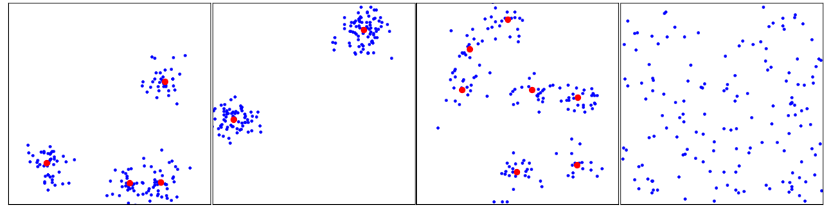
To explore the effect of variability in the training datasets, we consider a specific family of instance distributions (tasks), indexed by the following parameters: the graph size , the number of modes , the vehicle capacity and the scale . Given these parameters, an instance is generated by the following process. When : first, points, called the modes, are independently sampled by an ad-hoc process which tends to spread them evenly in the unit square; then points are independently sampled from a balanced mixture of Gaussian components centered at the modes, sharing the same diagonal covariance matrix, meant to keep the generated points within relatively small clusters around the modes; finally, the node coordinates are rescaled by a factor . When : the points are instead directly sampled uniformly in the unit square then rescaled by . Additionally, in the case of the CVRP problem, the depot is chosen randomly, the vehicle capacity is fixed to and customer demands are generated as in [20]. Examples of spatial node distributions for various TSP tasks are displayed in Figure 1.
3.2 Measuring the impact of generalization on performance
To measure the performance of different algorithms on a given task, we sample a set of test instances from that task and apply each algorithm to each of these instances. Since the average length of the resulting tours is biased towards longer lengths, we measure instead the average “gap” with respect to reference tours. For the TSP, reference is provided by the Concorde solver [1], which is exact, so what we report is the true optimality gap; for the CVRP, we use the solutions computed by the state-of-the-art LKH heuristic solver [10], which returns high-quality solutions at the considered instance sizes (near optimality).
We measure the performance (gap) deterioration on generalization of the reinforcement learning based Attention Model of [14], subsequently abbreviated as AM, and the supervised Graph Convolutional Network model of [11], subsequently abbreviated as GCN. We consider several classes of tasks of the form obtained by varying, in each class, only one of the parameters11 1 Except with CVRP where, as in previous work [20], changes to and are coupled. . For each class and each task in that class, we train each model on that task only and test it on each of the tasks in the same class, thus including the training one. The main results for the AM model are reported in Table 2.
As already observed in several papers, varying the number of nodes degrades the performance (columns (a) and (d)). Interestingly, varying the number of modes only also has a negative impact (columns (b) and (e)), and the same holds when varying the scaling of the node coordinates in the TSP (column (c)) or the vehicle capacity in the CVRP (column (f)). Similar results of performance degradation on generalization of the GCN model are given in Table 2 for TSP. These results confirm the drastic lack of generalization between the models, even on seemingly closely related instance distributions. In the next section, we propose an approach to tackle this problem.
| 0.08 | 1.78 | 22.61 | 1.47 | 32.17 | 2.74 | 1.48 | 282.55 | 292.39 | |||
| 0.35 | 0.52 | 2.95 | 26.38 | 1.86 | 7.32 | 32.84 | 1.44 | 13.83 | |||
| 3.78 | 2.33 | 2.26 | 6.91 | 6.01 | 2.0 | 98.62 | 7.12 | 1.53 | |||
| (a) () | (b) () | (c) () | |||||||||
| 4.52 | 12.61 | 20.23 | 4.39 | 51.02 | 102.07 | 5.83 | 8.25 | 12.23 | |||
| 7.99 | 6.93 | 8.47 | 5.67 | 6.32 | 16.14 | 6.13 | 7.37 | 9.39 | |||
| 12.90 | 9.75 | 7.11 | 14.91 | 8.67 | 7.85 | 12.27 | 8.56 | 7.99 | |||
| (d) () | (e) () | (f) () | |||||||||
| 1.83 | 38.66 | 77.31 | 5.05 | 35.86 | 26.01 | 5.10 | 28.15 | 32.46 | |||
| 22.05 | 5.10 | 43.76 | 35.40 | 6.96 | 28.71 | 272.58 | 5.23 | 25.41 | |||
| 43.86 | 37.26 | 14.79 | 32.74 | 36.29 | 5.48 | 289.51 | 66.28 | 5.46 | |||
| (a) () | (b) () | (c) () | |||||||||
4 Meta-learning of NCO heuristics

The goal of this paper is to introduce an NCO approach capable of out-of-distribution generalization for a given CO problem. Since NCO methods tend to perform well on fixed instance distributions, our strategy to promote out-of-distribution generalization is to modify the way the model is trained without changing its architecture.
Concretely, given a CO problem (e.g. the TSP), we assume that we have a prior over the relevant tasks (instance distributions), possibly based on historical data. For instance, we may know that the customers in our TSP are generally clustered around city centers, but without knowing how many clusters. Our underlying assumption is that it easier and more realistic to obtain a prior distribution on target tasks, rather than the target task itself. We propose to first train a model to learn an efficient heuristic on a sample of tasks (e.g. TSP instances with different numbers of modes). Then, considering a new unseen task (unseen number of modes), we would use a limited number of samples (few-shots) from that task to specialize the learned heuristic and maximize its performance on it. Fig. 2 illustrates our proposed approach.
Formally, given an NCO model with parameters and a distribution of tasks , our goal is to compute a parameter such that, given an unseen task with associated loss , after gradient updates, the fine-tuned parameter minimizes , i.e.
| (1) |
where is the fine-tuned parameter after gradient updates of using batches of instances from task . Problem (1) can be viewed as a few-shot meta-learning optimization problem. We approach it in a model-agnostic fashion by leveraging the generic Reptile meta-learning algorithm [21]. Given a task distribution, Reptile is a surprisingly simple algorithm to learn a model that performs well on unseen tasks of that distribution. Compared to the seminal MAML framework [6], Reptile is a first-order method that does not differentiate through the fine-tuning process at train time, making it feasible to work with higher values of . And we observed experimentally that in our context, to fine-tune a model to a new task, we need up to steps, which is beyond MAML’s practical limits. Furthermore, since Reptile uses only first-order gradients with a very simple form, it is more efficient, both in terms of computation and memory. Using Reptile, we meta-train each model on the given task distribution to obtain an effective initialization of the parameters, which can subsequently be adapted to a new target task using a limited number of fine-tuning samples from that task.
The first step to optimize Eq. 1 consists of updates of task specific parameters for a task as follows:
| (2) |
In the above equation, the hyper-parameter controls the learning rate. Then, using the updated parameters obtained at the end of the steps, we update the meta-parameter as follows:
| (3) |
This is essentially a weighted combination of the updated task parameters and previous model parameters . The parameter can be interpreted as a step-size in the direction of the Reptile “gradient” . It controls the contribution of task specific parameters to the overall model parameters. We iterate over by computing Eq. 3 for different tasks and then using it for optimizing Eq. 1.
Scheduling : first specialize then generalize. As mentioned above, parameter controls the contribution of the task specific loss to the global meta parameters update in Eq. 3. A high value of leads to overfitting on the training task while a low value leads to inefficient learning of the task itself. In order to tackle such scenario, in this work we utilize a simple decaying schedule for which starts close to 1 (i.e. the meta-parameters are updated to the fine-tuned ones) and tends to 0 as the training proceeds, thus stabilizing the meta-parameter that is more likely to work well for all tasks.
Fine-tuning for target adaptation: Once the model is meta-trained on a diverse set of tasks, given a new task , we initialize the target task parameters to the value of the meta-trained model and do a number a fine-tuning steps to get the specialized model for the new task. Essentially,
| (4) |
We can now detail the meta-training procedure of NCO models for the TSP and CVRP problems over our two state-of-the-art reinforcement learning (AM) and supervised learning (GCN) approaches to NCO heuristic learning. For simplicity, we use as default problem the TSP in this section, while the adaptation of the algorithms for the CVRP is presented in Sec. A.2 in Supplementary Material.
4.1 Meta-learning of RL-based NCO heuristics (AM model)
The RL based model of [14] (AM) consists of learning a policy that takes as input a graph representing the TSP instance and outputs the solution as a sequence of graph nodes. The policy is parameterized by a neural network with attention based encoder and decoder [26] stages. The encoder computes nodes and graph embeddings; using these embeddings and a context vector, the decoder produces the sequence of input nodes in an auto-regressive manner.
In effect, given a graph instance with nodes, the model produces a probability distribution from which one can sample to get a full solution in the form of a permutation of . The policy parameter is optimized to minimize the loss: ,
where is the cost (or length) of the tour . The REINFORCE [29] gradient estimator is used: .
As in [14], we use as baseline the cost of a greedy rollout of the best model policy, that is updated periodically during training.
Meta-training of AM:
Algorithm 1 describes our approach for meta-training the AM model for the TSP problem. For simplicity, the distribution of tasks that we consider here is uniform over a finite fixed set of tasks. Otherwise, one just needs to define the task-specific baseline parameters on the fly when a task is sampled for the first time. The training consists of repeatedly sampling a task (line 3), doing update of the meta-parameters using samples from that task to get fine-tuned parameters , then updating the meta-parameters as a convex combination of their previous value and the fine-tuned value (line 15). Note that the baseline need not be updated at each step (line 12), but only periodically, to improve the stability of the gradients.
4.2 Meta-learning of supervised NCO heuristics (GCN model)
The supervised model of [11] (GCN) consists of a Graph Convolution Network that takes as input a TSP instance as a graph and outputs, for each edge in , predicted probabilities of being part of the optimal solution. It is trained using a weighted binary cross-entropy loss between the predictions and the ground-truth solution provided by the exact solver Concorde [1]:
| (5) |
where and are class weights meant to compensate the inherent class imbalance, and is the batch size. The predicted probabilities are then used either to greedily construct a tour, or as an input to a beam search procedure. For simplicity, and because we are interested in the learning component of the method, we only consider here the greedy version.
Meta-training of GCN: Algorithm 2 in Supplementary Material describes our approach for meta-training the GCN model. In contrast to Algorithm 1, we need here to fix the training tasks since the ground-truth optimal solutions must be precomputed in this supervised learning framework.
5 Experiments
The goal of our experiments is to demonstrate the effectiveness of meta-learning for achieving generalization in NCO. More precisely, given a prior distribution of tasks, we aim to answer the following questions: (i) How does the (fine-tuned) meta-trained NCO models perform on unseen tasks, in terms of optimality gaps and sample efficiency? (ii) How does the meta-trained models perform on unseen tasks that are interpolated or extrapolated from the training tasks? (iii) How effective is our proposed decaying step-size strategy in the Reptile meta-learning algorithm for our NCO tasks?
Experimental setup. Experiments were performed on a pool of machines running Intel(R) CPUs with 16 cores, 256GB RAM under CentOS Linux 7, having Nvidia Volta V100 GPUs with 32GB GPU memory. All the models were trained for 24 hours on 1 GPU. The detailed hyperparameters are presented in Sec. A.4 of the Supp. Mat.. Our code and datasets are available at: https://anonymous.4open.science/r/meta-NCO
Task distributions. For the TSP (resp. CVRP) experiments, we consider four task distributions (Section 3.1) which are obtained from (resp. ) as follows: (i) a var-size distribution is obtained by varying only, and for training tasks within this distribution we use ; (ii) var-mode distribution by varying only, and for training ; (iii) mixed-var distribution by varying both and and training with ; and (iv) only for CVRP: var-capacity distribution by varying only, for training . As test tasks, we use values that are both within the training tasks range to evaluate the interpolation performance (e.g. for (ii)) and outside to evaluate the extrapolation performance (e.g. for (i)). More details about the distributions are presented in Sec. A.3 of the Supp. Mat.
Datasets. We generate synthetic TSP and CVRP instances, according to the previously described task distributions. For AM training, samples are generated on demand while for the GCN model, we generate for each task a training set of 1M instances, a validation and test set of 5K instances each and use the Concorde solver [1] and LKH [10] to get the associated ground-truth solutions for TSP and CVRP respectively (as was done in the original work). In order to fine-tune the meta-trained models, we sample a set of instances from the new task, containing either 3K (AM) or 1K (GCN) samples; these numbers were chosen as approximately and of the number of samples used during the 24 hours training of the AM and GCN models respectively (see details in Sec. A.5 in Supp. Mat.). In addition to synthetic datasets, we evaluate our models on the realistic datasets: TSPlib and CVRPlib. The precise settings and results are presented in Section 5.1.
Models. We use the AM-based heuristics of [14] for TSP and CVRP. For the GCN model, we use the model provided by [11] for the TSP and its adaptation by [15] for the CVRP. For a given task distribution (e.g. variable-size) we consider the following models:
- •
- •
multi-AM (resp. multi-GCN): the AM (resp. GCN) model trained with instances coming equiprobably from the training tasks. E.g. for the variable-mode distribution, we denote this model multi-AM-M (resp. multi-GCN-M).
- •
oracle-AM (resp. oracle-GCN): original AM (resp. GCN) model trained on the test instance distribution, that is unseen during training of both the meta and multi models. Note that the meta-models are not meant to improve over the oracles’ performance, although we will see that it happens sometimes.
To simplify the notations, we only explicitly differentiate between TSP and CVRP if it is not clear from the context. Since we are interested in the generalization of the neural models, regardless of the final decoding step (greedy, sampling, beam-search, etc), we use a simple greedy decoding for all the models. Besides, because our training is restricted to 24 hours for all the models (which is sufficient to ensure convergence of the training, see Fig 3 of Supp. Mat.), the results may not be as good are those reported in the original papers. To evaluate the impact of the meta-training on generalization when everything else fixed, we focus on the relative gap in performance between the different models.
Generalization performance: To evaluate the generalization ability of the meta-trained models, we present in Table 3 the performance of the different models at 0-shot generalization (=0) and after =50 fine-tuning steps, for various pairs of prior task distributions and unseen test tasks. We observe that in all cases the fine-tuned meta-AM clearly outperforms the fine-tuned baseline multi-AM and even outperforms the oracle-AM model in 7 out of 12 tasks. Similar observations hold for the meta-GCN model: it is better both at 0-shot generalization and after fine-tuning than the multi-GCN baseline, and it outperforms the oracle in 2 out of 6 tasks. These results show that meta-AM is able to achieve impressive quality while using a negligible amount of training data of the target task compared to the original model (oracle-AM). More results on different target tasks as well as plots of the evolution of the performance with the number of fine-tuning steps are presented in Sec. A.7 of the Supp. Mat.
| TSP | Tasks | var-size distrib. | var-mode distrib. | mixed-var distrib. | |||
|---|---|---|---|---|---|---|---|
| Models | N=100 | N=150 | M=3 | M=8 | (N,M)=(40,6) | (N,M)=(40,8) | |
| oracle-AM | 5.96% | 12.08% | 1.87 % | 1.83% | 2.00% | 1.83% | |
| Farthest Ins.[23] | 7.48% | 8.55% | 2.08% | 2.27% | 16.32% | 11.70% | |
| multi-AM (=0) | 8.73% | 14.40% | 5.57% | 6.20% | 10.70% | 15.18% | |
| multi-AM (=50) | 7.25% | 10.87% | 5.26% | 4.60% | 7.59% | 10.26% | |
| meta-AM (=0) | 7.10% | 12.25% | 1.96% | 2.16% | 2.41% | 3.50% | |
| meta-AM (=50) | 5.58% | 9.84% | 1.82% | 1.70% | 2.15% | 2.93% | |
| CVRP | Tasks | var-size distrib. | var-mode distrib. | var-capacity distrib. | |||
| Models | N=100 | N=150 | M=3 | M=8 | C=20 | C=50 | |
| oracle-AM | 8.71% | 11.56% | 6.32 % | 7.85% | 5.83% | 8.01% | |
| multi-AM (=0) | 18.82% | 18.76% | 7.87% | 12.65% | 9.15% | 14.28% | |
| multi-AM (=50) | 9.18% | 11.41% | 7.58% | 10.20% | 8.09% | 10.16% | |
| meta-AM (=0) | 11.50% | 16.42% | 6.05% | 9.38% | 6.26% | 8.94% | |
| meta-AM (=50) | 7.71% | 9.91% | 5.96% | 8.45% | 6.05% | 8.82% | |
| TSP | Tasks | var-size distrib. | var-mode distrib. | mixed-var distrib. | |||
| Models | N=80 | N=100 | M=3 | M=8 | (N,M)=(40,6) | (N,M)=(40,8) | |
| oracle-GCN | 12.34% | 14.72% | 7.65% | 6.21% | 6.06% | 3.22% | |
| multi-GCN (K=0) | 28.40% | 34.29% | 9.22% | 7.89% | 28.01% | 5.05% | |
| multi-GCN (K=50) | 16.73% | 30.80% | 8.43% | 6.59% | 5.99% | 4.42% | |
| meta-GCN (K=0) | 19.70% | 32.01% | 8.19% | 7.32% | 6.62% | 3.72% | |
| meta-GCN (K=50) | 13.73% | 18.42% | 7.72% | 6.45% | 5.67% | 3.17% | |
Time and sample efficiency. For a complete evaluation of the proposed meta-training and then fine-tuning approach for NCO, we discuss here its cost in terms of the fine-tuning time and number of training samples from the target task required to reach the optimality gaps of Table 3. Regarding the fine-tuning time, the 50 fine-tuning steps took 2 to 6m for meta-AM and 43s to 2m for meta-GCN. Further, generating the 1k optimal solutions for fine-tuning the supervised meta-GCN model took up to 17m for TSP150 and 20h for CVRP150. These values should be compared to the generation time of the 1M solutions for training the oracle-GCN model on the target instance distribution. Besides, for example for TSP with , we observed that oracle-AM needs around 23 hours and more than Million samples of the target task to reach the optimality gap of . On the other hand, meta-AM-M only used samples from the target task and achieved a better performance after a few fine-tuning steps and less than 6 minutes. The baseline approach multi-AM-M was still far away at optimality gap after fine-tuning. Similar observations hold for meta-GCN on TSP with : Oracle-GCN-M needs around 22 hours and 1 Million instances of labeled data (with optimal solutions) to reach an optimality gap of 7.72%, while meta-GCN-M reaches the same performance in just 16 seconds, using 500 solved instances. Hence, one model trained using our prescribed meta-learning approach can be used to adapt to different tasks efficiently within a short span of time and using few fine-tuning samples. More details on training time and number of samples used for different tasks can be found in the Table 7 of the Supp. Mat. Additionally, Fig. 3 in the Supp. Mat. presents the performance of different models w.r.t time on test tasks during their course of training.
5.1 Experiments on real-world datasets
To evaluate the performance of our approach beyond synthetic datasets, we ran experiments on two well-established OR datasets: TSPlib22 2 http://comopt.ifi.uni-heidelberg.de/software/TSPLIB95/ and CVRPlib33 3 http://vrp.atd-lab.inf.puc-rio.br/index.php/en/. From TSPlib we took the instances of size to nodes. Note that in this context, the RL approach which does not rely on labeled data for fine-tuning is more appropriate. Since these instances are heterogeneous (i.e. no clear underlying distribution), we directly fine-tune the models on each test instance. This is an extreme case of our setting where the target task is reduced to 1 instance. We tested the models that were (meta-)trained on the variable-size distribution of synthetic instances for meta-AM and multi-AM. For AM we took the pretrained model on graphs of size =100. Because of space limitation, we grouped the instances per size range and report in Table 4 the average optimality gap obtained after =100 fine-tuning steps, taking s to m (detailed per-instance results in Sec. A.8 of Supp Mat). Note that in this case we also fine-tune the AM model since it was not trained on the target instances distribution.
From CVRPlib we used the 106 instances of size up to 200 nodes. Since instances are grouped by sets, we apply our few-shot learning setting: fine-tuning for steps on approximately 10% of the instances of a set and testing on the rest. In Table 4, we report the average optimality gap over 5 random fine-tuning/test splits for each set. The results are consistent with our previous observations and illustrate the superior performance of our proposed meta-learning strategy in this realistic setting. It also shows that even if the prior task distribution is not perfect (in the sense that it does not include the target task), the meta-training gives a strong parameter initialization which one can fine-tune effectively on the target task.
| TSPlib | CVRPlib | |||||||
| Set A | Set B | Set E | Set P | Set X | ||||
| AM | ||||||||
| multi-AM | 13.00% | |||||||
| meta-AM | 5.95% | 5.91% | 13.22% | 3.56% | 5.07% | 5.03% | 11.87% | |
5.2 Ablation study
Fixed vs decaying step-size . In this section, we study the impact of our proposed decaying approach during meta-training. Specifically, Table 5 presents the results of using a standard fixed step-size versus a decaying . We see that the decaying version of meta-AM and meta-GCN outperforms the fixed one, both in terms of 0-shot generalization (i.e ) and after steps of fine-tuning. This supports our argument for performing task specialization in the beginning and generalization at the end of the meta-training procedure.
| Test task | Fine-tuning | decaying | ||||||
|---|---|---|---|---|---|---|---|---|
| meta-AM | before () | 9.91% | 8.33% | 7.52% | 6.94% | 6.63% | 7.10% | |
| after () | 7.83% | 6.50% | 6.03% | 5.95% | 5.96% | 5.58% | ||
| before () | 5.99% | 3.07% | 3.38% | 2.35% | 2.52% | 2.16% | ||
| after () | 4.78% | 2.27% | 2.63% | 1.87% | 2.04% | 1.70% | ||
| meta-GCN | before () | 13.08% | 11.90% | 11.92% | 12.90% | 10.11% | 6.01% | |
| after () | 9.86% | 8.27% | 9.52% | 10.80% | 13.16% | 5.71% | ||
| before () | 9.78% | 8.81% | 9.20% | 11.05% | 11.96% | 7.39% | ||
| after () | 8.32% | 7.37% | 8.23% | 9.76% | 11.80% | 6.45% |
6 Conclusion
In this paper, we address the well-recognized generalization issue of end-to-end NCO methods. In contrast to previous works that aim at having one model perform well on various instance distributions, we propose to learn a model that can efficiently adapt to different distributions of instances. To implement this idea, we recast the problem in a meta-learning framework, and introduce a simple yet generic way to meta-train NCO models. We have shown experimentally that our proposed meta-learned RL-based and SL-based NCO heuristics are indeed robust to a variety of distribution shifts for two CO problems. Additionally, the meta-learned models also achieve superior performance on realistic datasets. We show that our approach can push the boundary of the underlying NCO models by solving instances with up to 200 nodes when the models are trained with only up to 50 nodes. While the known limitations of the underlying models (esp. the attention bottleneck, and fully-connected GCN) prevent tackling much larger problems, our approach could be applied for other models. Finally note that there are several possible levels of generalization in NCO. In this paper, we have mostly focused on improving the generalization to instance distributions for a fixed CO problem. To go further, one could investigate the generalization to other CO problems. For this more ambitious goal, domain adaptation approaches, which explicitly account for the domain shifts (e.g. using adversarial-based techniques [25]) could be an interesting direction to explore.
References
- [1] David. Applegate, Robert. Bixby, Vašek Chvátal and William. Cook “The Traveling Salesman Problem: A Computational Study” In The Traveling Salesman Problem Princeton University Press, 2011 URL: https://www.degruyter.com/document/doi/10.1515/9781400841103/html?lang=en
- [2] Irwan Bello et al. “Neural Combinatorial Optimization with Reinforcement Learning”, 2017 arXiv: http://arxiv.org/abs/1611.09940
- [3] Yoshua Bengio, Andrea Lodi and Antoine Prouvost “Machine Learning for Combinatorial Optimization: A Methodological Tour d’horizon” In European Journal of Operational Research 290.2 Elsevier, 2021, pp. 405–421 URL: https://ideas.repec.org/a/eee/ejores/v290y2021i2p405-421.html
- [4] Quentin Cappart et al. “Combinatorial Optimization and Reasoning with Graph Neural Networks”, 2021 arXiv: http://arxiv.org/abs/2102.09544
- [5] William. Cook, William. Cunningham, William. Pulleyblank and Alexander Schrijver “Combinatorial Optimization” New York: Wiley-Interscience, 1997
- [6] Chelsea Finn, Pieter Abbeel and Sergey Levine “Model-Agnostic Meta-Learning for Fast Adaptation of Deep Networks” In Proceedings of the 34th International Conference on Machine Learning - Volume 70, ICML’17 Sydney, NSW, Australia: JMLR.org, 2017, pp. 1126–1135
- [7] Matteo Fischetti and Andrea Lodi “Heuristics in Mixed Integer Programming” In Wiley Encyclopedia of Operations Research and Management Science American Cancer Society, 2011 URL: https://onlinelibrary.wiley.com/doi/abs/10.1002/9780470400531.eorms0376
- [8] Zhang-Hua Fu, Kai-Bin Qiu and Hongyuan Zha “Generalize a Small Pre-trained Model to Arbitrarily Large TSP Instances”, 2020 arXiv: http://arxiv.org/abs/2012.10658
- [9] Dobrik Georgiev and Pietro Liò “Neural Bipartite Matching”, 2020 arXiv: http://arxiv.org/abs/2005.11304
- [10] Keld Helsgaun “An Extension of the Lin-Kernighan-Helsgaun TSP Solver for Constrained Traveling Salesman and Vehicle Routing Problems”, 2017, pp. 60
- [11] Chaitanya. Joshi, Thomas Laurent and Xavier Bresson “An Efficient Graph Convolutional Network Technique for the Travelling Salesman Problem”, 2019 arXiv: http://arxiv.org/abs/1906.01227
- [12] Chaitanya. Joshi, Thomas Laurent and Xavier Bresson “On Learning Paradigms for the Travelling Salesman Problem”, 2019 arXiv: http://arxiv.org/abs/1910.07210
- [13] Chaitanya. Joshi et al. “Learning TSP Requires Rethinking Generalization”, 2020 arXiv: http://arxiv.org/abs/2006.07054
- [14] Wouter Kool, Herke van Hoof and Max Welling “Attention, Learn to Solve Routing Problems!”, 2019 URL: https://openreview.net/forum?id=ByxBFsRqYm
- [15] Wouter Kool, Herke van Hoof, Joaquim Gromicho and Max Welling “Deep Policy Dynamic Programming for Vehicle Routing Problems”, 2021 arXiv: http://arxiv.org/abs/2102.11756
- [16] Sirui Li, Zhongxia Yan and Cathy Wu “Learning to Delegate for Large-Scale Vehicle Routing” In Advances in Neural Information Processing Systems 34 Pre-Proceedings, 2021 URL: https://openreview.net/forum?id=rm0I5y2zkG8
- [17] Zhuwen Li, Qifeng Chen and Vladlen Koltun “Combinatorial Optimization with Graph Convolutional Networks and Guided Tree Search” In Advances in Neural Information Processing Systems 31 Curran Associates, Inc., 2018, pp. 537–546 URL: http://papers.nips.cc/paper/7335-combinatorial-optimization-with-graph-convolutional-networks-and-guided-tree-search.pdf
- [18] Michal Lisicki, Arash Afkanpour and Graham. Taylor “Evaluating Curriculum Learning Strategies in Neural Combinatorial Optimization”, 2020 arXiv: http://arxiv.org/abs/2011.06188
- [19] Vinod Nair, Dj Dvijotham, Iain Dunning and Oriol Vinyals “Learning Fast Optimizers for Contextual Stochastic Integer Programs” In UAI 2018, 2018
- [20] MohammadReza Nazari, Afshin Oroojlooy, Lawrence Snyder and Martin Takac “Reinforcement Learning for Solving the Vehicle Routing Problem” In Advances in Neural Information Processing Systems 31 Curran Associates, Inc., 2018 URL: https://proceedings.neurips.cc/paper/2018/hash/9fb4651c05b2ed70fba5afe0b039a550-Abstract.html
- [21] Alex Nichol, Joshua Achiam and John Schulman “On First-Order Meta-Learning Algorithms”, 2018 arXiv: http://arxiv.org/abs/1803.02999
- [22] Sachin Ravi and Hugo Larochelle “OPTIMIZATION AS A MODEL FOR FEW-SHOT LEARNING”, 2017, pp. 11
- [23] Daniel. Rosenkrantz, Richard. Stearns and Philip. Lewis “An Analysis of Several Heuristics for the Traveling Salesman Problem” In Fundamental Problems in Computing: Essays in Honor of Professor Daniel J. Rosenkrantz Dordrecht: Springer Netherlands, 2009, pp. 45–69 URL: https://doi.org/10.1007/978-1-4020-9688-4_3
- [24] Jürgen Schmidhuber “Evolutionary Principles in Self-Referential Learning, or on Learning How to Learn: The Meta-Meta-… Hook”, 1987 URL: https://mediatum.ub.tum.de/813180
- [25] Eric Tzeng, Judy Hoffman, Kate Saenko and Trevor Darrell “Adversarial Discriminative Domain Adaptation”, 2017, pp. 7167–7176 URL: https://openaccess.thecvf.com/content_cvpr_2017/html/Tzeng_Adversarial_Discriminative_Domain_CVPR_2017_paper.html
- [26] Ashish Vaswani et al. “Attention Is All You Need”, 2017 arXiv: http://arxiv.org/abs/1706.03762
- [27] Petar Veličković et al. “Neural Execution of Graph Algorithms”, 2019 URL: https://openreview.net/forum?id=SkgKO0EtvS
- [28] Oriol Vinyals, Meire Fortunato and Navdeep Jaitly “Pointer Networks” In Advances in Neural Information Processing Systems 28 Curran Associates, Inc., 2015, pp. 2692–2700 URL: http://papers.nips.cc/paper/5866-pointer-networks.pdf
- [29] Ronald. Williams “Simple Statistical Gradient-Following Algorithms for Connectionist Reinforcement Learning” In Machine Learning 8.3, 1992, pp. 229–256 URL: https://doi.org/10.1007/BF00992696
- [30] D.H. Wolpert and W.G. Macready “No Free Lunch Theorems for Optimization” In IEEE Transactions on Evolutionary Computation 1.1, 1997, pp. 67–82 URL: http://ieeexplore.ieee.org/document/585893/
- [31] Giulia Zarpellon, Jason Jo, Andrea Lodi and Yoshua Bengio “Parameterizing Branch-and-Bound Search Trees to Learn Branching Policies”, 2021 arXiv: http://arxiv.org/abs/2002.05120
Appendix A Supplementary Material
A.1 Meta-training of the GCN model
Algorithm 2 summarizes the main steps of meta-training the GCN model:
A.2 Meta-training for CVRP
Since the Attention model [Kool et al., 2019] was proposed for both the TSP and CVRP (and other routing problems) and the GCN model [Joshi et al., 2019a] originally proposed for the TSP was adapted by [Kool et al., 2021] to the CVRP, we update the model parameters dimension and input to take into account the depot node, the demand and vehicle capacity, the cost function, greedy rollout baseline and losses as in the original papers. With these updated parameters and functions, Algorithms 1 and 2 remain the same for meta-training the Attention model and the GCN model respectively, for the CVRP.
A.3 Task distribution datasets
We summarise the datasets that were generated and that we will make available to hopefully be helpful to the NCO community for evaluating the generalisation ability of their models. In Section 3.1 of the paper, we have described how we generate tasks (or instance distributions) of the form , for the TSP and the CVRP. With the default values , we have created three collections of datasets for the TSP:
- •
Varying number of nodes:
- •
Varying number of modes
- •
Varying scale
Similarly, with default values , we have generated three collections of datasets for the CVRP:
- •
Varying both number of nodes and associated capacity:
- •
Varying capacity
- •
Varying number of modes
For each task, we have generated 1M training instances and K validation and test instances. The solutions were computed using the Concorde solver [Applegate et al., 2006] for TSP and LKH solver [Helsgaun, 2017] for CVRP. In total, we have generated 16 datasets for the TSP and 16 for the CVRP. Using a 32 cores CPU, it took on average about 10 hours per dataset for TSP and 10 days for the CVRP.
Note that the varying-scale dataset is trivially obtained from the original dataset with scale 1 and the solutions are unchanged. Although one can easily normalise the coordinates in this case and avoid any distribution shift in scale, we have used these datasets as an additional illustration of the sensitivity of the models.
A.4 Experimental details
Hyper-parameters: For both the Attention model and GCN model, we reuse as much as possible the default hyper-parameters of the original papers. For meta-AM, during meta-training we set , and ; meta-GCN,during meta-training we set , , between and . We already discussed the benefit of our proposed decaying parameter in the main paper. Here, we study the impact of the other meta-training specific hyper-parameter on the performance. Specifically, in Table 6 we show the impact of the number of fine-tuning steps used during the training of the meta-models meta-AM and meta-GCN, on their test performance.
| Test task | Fine-tuning | Default | ||||||||
|---|---|---|---|---|---|---|---|---|---|---|
| meta-AM | before | 10.76% | 7.41% | 6.87% | 6.75% | 5.79% | 6.05% | 6.04% | 7.10% | |
| after | 8.13% | 6.52% | 5.91% | 5.92% | 5.26% | 5.40% | 5.33% | 5.58% | ||
| before | 3.20% | 3.46% | 3.16% | 3.26% | 2.47% | 2.09% | 2.99% | 2.16% | ||
| after | 2.50% | 2.49% | 2.43% | 2.81% | 2.00% | 1.76% | 2.28% | 1.70% | ||
| meta-GCN | before | 19.03% | 16.32% | 10.32% | 10.96% | 10.13% | 11.70% | 11.00% | 6.01% | |
| after | 19.29% | 14.44% | 9.86% | 10.53% | 9.63% | 11.21% | 10.98% | 5.71% | ||
| before | 19.33% | 13.67% | 9.28% | 8.59% | 10.13% | 9.85% | 9.86% | 6.42% | ||
| after | 17.49% | 12.69% | 8.74% | 8.43% | 9.71% | 9.66% | 9.74% | 6.06% |
A.5 Sample efficiency
As mentioned in Sec. 5 of the main paper, the efficiency of our proposed methods meta-AM and meta-GCN should be viewed keeping in mind the number of training samples of the target task used for training a model from scratch(oracle). As discussed earlier, for meta-AM we use only samples from the target task during fine-tuning. This is way lower than millions of samples used for training a model from scratch(oracle-AM) as can be seen in Table 7. As we see, in both cases, the number of samples of the target task used by meta-AM are of orders of magnitude smaller than oracle-AM.
| Scale factor | |||||||||||
| oracle-AM | 46.2 | 38.1 | 33.1 | 25.2 | 31.8 | 30.0 | 26.1 | 29.1 | 78.1 | 78.3 | |
| 6.49 | 7.87 | 9.06 | 11.9 | 9.43 | 10.0 | 11.5 | 10.3 | 3.84 | 3.83 | ||
| (a) Travelling Salesman Problem(TSP) | |||||||||||
| Scale factor | |||||||||||
| oracle-AM | 28.2 | 24.6 | 21.0 | 16.0 | 21.2 | 22.1 | 16.0 | 15.0 | 37.3 | 34.1 | |
| 1.06 | 1.22 | 1.43 | 1.88 | 1.42 | 1.36 | 1.88 | 2.00 | 0.80 | 0.88 | ||
| (b) Capacitated Vehicle Routing Problem(CVRP) | |||||||||||
A.6 Performance vs training time
In this section we study the performance of different models evaluated on the test datasets during their course of training. In Fig 3, we observe that the improvement for all models becomes very slow at the end. Although AM will improve slowly after the 24h mark, the meta fine-tuned meta-model is much faster to reach a better performance.


A.7 Additional Results
meta-AM Generalization: Evolution of performance at different fine-tuning steps: In the main paper, we showed the results for different datasets at fine-tuning steps and . In this section, in Fig. 4 and 5 we show the evolution of the optimality gaps at different fine-tuning steps varying from to . Apart from the test datasets shown in main paper, we also present additional results (meta-AM) on additional tasks not shown in main paper in Fig. 6 and 7. Similar to the observations made in the main paper, we see that in most cases meta-AM (blue) clearly generalizes better than the baseline multi-AM (green) and even outperforms the oracle-AM model. Similar observations can be made for meta-AM model for CVRP in Figure 7. In all cases, meta-AM outperforms both multi-AM and oracle-AM.
meta-GCN Generalization: In Sec.5 of the main paper, we have presented results of the meta-GCN model on TSP. In this section, we show the evolution of performance of the meta-GCN model in terms of optimality gap. In Fig. 9 for TSP, for the var-mode setting for meta-GCN trained on we observe that in all cases, meta-GCN performs better than the baseline multi-GCN and in 3 out of 4 cases, it even outperforms the oracle-GCN model. For the var-size setting, for meta-GCN trained on , we observe that meta-GCN outperforms multi-GCN when the number of fine-tuning steps are less. However, we can see that when the number of fine-tuning steps increases, the optimality gap of multi-GCN is better even though its test loss is higher(see Fig. 8). A possible reason for this behaviour is our use of greedy decoding and instead of the beam-search/sampling-based decoding. For the mixed-var distribution setting, for the meta-GCN model trained on , we observe that for and , meta-GCN outperforms multi-GCN and the oracle-GCN model in terms of optimality gap.
-0.1in
A.8 TSPlib: Instance wise results
In this section we present the results for all the TSPlib instances used in Sec. 5.1 of the main paper. In Table. 8 we observe that in most cases, especially the larger size instances, our proposed meta-AM framework outperforms other baselines by a significant margin.
| Instance | AM() | multi-AM() | meta-AM() |
|---|---|---|---|
| eil51 | 2.465 | 6.459 | 2.858 |
| berlin52 | 16.643 | 13.65 | 2.942 |
| st70 | 2.621 | 7.241 | 3.729 |
| eil76 | 5.233 | 7.688 | 6.202 |
| pr76 | 1.921 | 7.732 | 2.417 |
| rat99 | 14.224 | 25.941 | 13.511 |
| kroA100 | 13.413 | 17.705 | 5.08 |
| kroE100 | 9.157 | 9.557 | 6.963 |
| rd100 | 5.718 | 6.253 | 1.139 |
| kroC100 | 8.232 | 14.928 | 10.928 |
| kroB100 | 10.718 | 14.133 | 9.199 |
| kroD100 | 11.925 | 12.152 | 6.412 |
| eil101 | 5.862 | 9.291 | 5.228 |
| lin105 | 6.538 | 19.71 | 5.248 |
| pr107 | 5.348 | 8.698 | 7.353 |
| pr124 | 4.724 | 8.736 | 0.927 |
| bier127 | 12.281 | 23.628 | 7.312 |
| ch130 | 5.376 | 12.087 | 2.068 |
| pr144 | 11.163 | 14.412 | 5.909 |
| ch150 | 7.978 | 9.107 | 8.268 |
| kroA150 | 9.664 | 14.808 | 8.802 |
| kroB150 | 10.771 | 12.75 | 7.96 |
| pr152 | 10.201 | 9.848 | 5.038 |
| u159 | 10.95 | 21.465 | 7.317 |
| rat195 | 16.617 | 30.093 | 17.059 |
| d198 | 42.953 | 54.282 | 23.314 |
| kroA200 | 10.398 | 19.773 | 13.87 |
| kroB200 | 12.966 | 20.761 | 12.734 |
A.9 Visualisation of some solutions
Figure 11 shows the solutions computed by 3 models on a few TSP instances sampled from , one per row. The first column (black) corresponds to meta-AM with no fine-tuning, trained for 24h on 1 million instances from (hence not including the target distribution). The second column (blue) corresponds to the same model, after steps of fine tuning on instances drawn from the target distribution. The last column (green) corresponds to the true optimal results as obtained by Concorde.