∎

Composition of Relational Features with an Application to Explaining Black-Box PredictorsJournal: Machine Learning

Ashwin Srinivasan^∗ A Baskar Tirtharaj Dash^† Devanshu Shah Affiliation: A. Srinivasan Affiliation: A. Srinivasan Affiliation: A. Baskar Affiliation: T Dash

Received: date / Accepted: date

Abstract

Three key strengths of relational machine learning programs like those developed in Inductive Logic Programming (ILP) are: (1) The use of an expressive subset of first-order logic that allows models that capture complex relationships amongst data instances; (2) The use of domain-specific relations to guide the construction of models; and (3) The models constructed are human-readable, which is often one step closer to being human-understandable. The price for these advantages is that ILP-like methods have not been able to capitalise fully on the rapid hardware, software and algorithmic developments fuelling current developments in deep neural networks. In this paper, we treat relational features as functions and use the notion of generalised composition of functions to derive complex functions from simpler ones. Motivated by the work of McCreath and Sharma (McCreath and Sharma 1998a; McCreath 1999) we formulate the notion of a set of $\mathrm{M}$ -simple features in a mode language $\mathrm{M}$ and identify two composition operators ( $\rho_{1}$ and $\rho_{2}$ ) from which all possible complex features can be derived. We use these results to implement a form of “explainable neural network’ called Compositional Relational Machines, or CRMs. CRMs are labelled directed-acyclic graphs. The vertex-label for any vertex $j$ in the CRM contains a feature-function $f_{j}$ and an continuous activation function $g_{j}$ . If $j$ is a “non-input” vertex, then $f_{j}$ is the composition of features associated with vertices in the direct predecessors of $j$ . Our focus is on CRMs in which input vertices (those without any direct predecessors) all have $\mathrm{M}$ -simple features in their vertex-labels. We provide a randomised procedure for constructing the structure of such CRMs, and a procedure for estimating the parameters (the $w_{ij}$ ’s $)$ using back-propagation and stochastic gradient descent. Using a notion of explanations based on the compositional structure of features in a CRM, we provide empirical evidence on synthetic data of the ability to identify appropriate explanations; and demonstrate the use of CRMs as ‘explanation machines’ for black-box models that do not provide explanations for their predictions.

Keywords:

Explainable Neural Networks, Relational Features, Inductive Logic Programming, Neuro-Symbolic Learning

1 Introduction

It has long been understood that choice of representation can make a significant difference to the efficacy of machine-based induction. A seminal paper by Quinlan 1979 demonstrates the increasing complexity of models constructed for a series of problems defined on a chess endgame, using a fixed representation consisting of 25 features (called properties in the paper). These features were identified manually (by him), and captured relations between the pieces and their locations in the endgame. Commenting on the increasing complexity of the models, he concludes:

“This immediately raises the question of whether these and other properties used in the study were appropriate. The answer is that they were probably not; it seems likely that a chess expert could develop more pertinent attributes …If the expert does his job well the induction problem is simplified; if a non-expert undertakes the definition of properties (as was the case here) the converse is true.”

Although Quinlan assumed the representation would be identified manually, the possibility of automatic identification of an appropriate representation was already apparent to Amarel 1968 a decade earlier: “An understanding of the relationship between problem formulation and problem solving efficiency is a prerequisite for the design of procedures that can automatically choose the most ‘appropriate’ representation of a problem (they can find a ‘point of view’ of the problem that maximally simplifies the process of finding a solution)”. In fact, by ‘choose’ what is probably meant is ‘construct’, if we are to avoid kicking Feigenbaum’s famous knowledge-acquisition bottleneck down the road from extracting models to extracting representations.

It has also been known that one way to construct representations automatically is through the use of neural networks. But extraction and re-use of these representations for multiple tasks have become substantially more common only recently, with the routine availability of specialised hardware. This has allowed the construction of networks in which adding layers of computation is assumed to result in increasingly complex representations (10s of layers are now common, but 100s are also within computational range). In principle, while a single additional layer is all that is needed (due to the Universal approximation theorems for neural networks (Hornik et al. 1989; Cybenko 1989; Pinkus 1999)), it is thought that the main benefit of the additional layers lies in constructing representations that are multiple levels of abstractions, allowing more efficient modelling. There are however 3 important issues that have surfaced: (1) Automatic construction of abstractions in this way requires a lot of data, often 100s of 1000s of examples; (2) The kinds of neural networks used for constructing abstractions depend on the type of data. For example, certain kinds of networks are used for text, others for images and so on: there is apparently no single approach for representation learning that can automatically adjust to the data type; and (3) The internal representations of data are opaque to human-readability, making it difficult to achieve the kind of understanding identified by Amarel.

Recent results with neural-based learning suggest the possibility of viewing representation learning as program synthesis. Of particular interest are methods like Dreamcoder (Ellis et al. 2021) that automatically construct programs for generating data, given some manually identified primitive functions represented in a symbolic form (Dreamcoder uses $\lambda$ -expressions for the primitive functions). A combination of generative and discriminative network models is used to direct the hierarchical construction of higher-level functions by compositions of lower-level ones. Compositions are generated and assessed for utility in inter-leaved phases of generate-and-test (called “Dream” and “Wake” phases), until the neural-machinery arrives at a small program, consisting the sequential composition of primitive- and invented functions. The final result is some approximation to the Bayesian MAP program for generating the data provided, assuming a prior preference for small programs. There are good reasons to look at this form of program-synthesis as a mechanism for automated representation learning: (a) Empirical results with programs like Dreamcoder show that it is possible to identify programs with small numbers of examples (the need for large numbers of examples is side-stepped by an internal mechanism for generating data in the Dream phase); (b) In principle, the symbolic language adopted for primitive functions ( $\lambda$ -expressions) and the mechanism of function composition is sufficiently expressive for constructing programs for data of any type; (c) The intermediate representations have clearly defined interpretations, based on functional composition. There are however some shortcomings. First, the primitive functions have to be manually identified. Secondly, the construction of new representations requires a combinatorial discrete search that is usually less efficient than those based on continuous-valued optimisation. Thirdly, the representation of $\lambda$ -expressions, although mathematically powerful, can prove daunting as a language for encoding domain-knowledge or for interpreting the results. Finally, the Dreamcoder-like approach for representation learning has only been demonstrated on very simple generative tasks of a geometric nature.

In this paper, we partially address these shortcomings by drawing on, and extending some results on representation developed in the area of Inductive Logic Programming (ILP). The main contributions of this paper are as follows:

(a) Conceptual: We develop the conceptual basis for a class of ‘simple’ relational features using a well-known specification language in ILP (mode-declarations). Additionally, we develop composition operators for deriving more complex relational features, and prove some completeness properties that apply to the use of the operators;
(b) Implementation: We use the concepts developed to specify and implement a form of neural network called Compositional Relational Machines, or CRMs. An important feature of these networks is that each node is identified with a clearly defined relational feature. This allows us to associate structured ‘explanations’ with each node in the network;
(c) Application: We present empirical results on 2 synthetic data that demonstrate the ability of CRMs to construct appropriate explanations; and results on using CRMs to act as ‘explanation machines’ for a state-of-the-art black-box predictor on 10 real-world datasets.

The rest of the paper is organised as follows: In Section 2 we provide a conceptual framework for relational features and their compositions. We use this framework to implement CRMs in Section 3. We provide empirical evaluation of CRMs as explanation machines in Section 4. Related work of immediate relevance to this paper are presented in Section 5. Concluding remarks are in in Section 6. The paper has several appendices that act as supporting material.

2 Relational Features and their Composition

In this paper, we are principally interested in specifying and combining relational features. For us, a $k$ -ary relational feature will be a function with $k$ terms as arguments. We will specify such a feature by $f:{\cal A}_{1}\times{\cal A}_{2}\times\cdots\times{\cal A}_{k}\rightarrow{\cal B}$ , where ${\cal A}_{1},{\cal A}_{2},\ldots,{\cal A}_{k},{\cal B}$ are some sets. For the most part in this paper, we will restrict ourselves to $k=1$ and ${\cal B}=\{0,1\}$ , although the results here can be generalised. We will denote this setting as $f:{\cal A}\rightarrow\{0,1\}$ , for some set ${\cal A}$ . A relational feature is defined in 2 steps. First, we represent the conditions under which the feature takes the value $1$ using a clause of the form:¹¹ 1 See Appendix A for a summary of logical syntax and concepts needed for this paper. We assume a logic with equality ( $=/2$ ).

C:~~\forall X~(p(X)\leftarrow\exists{\mathbf{Y}}{Body}(X,{\bf Y}))

or, simply:

C:~~(p(X)\leftarrow{Body}(X,{\bf Y}))

to mean the quantification as shown earlier. Here, the fixed predicate symbol $p(X)$ is called the head of $C$ , and ${Body}(X,\cdot)$ –the body of clause $C$ –is a conjunction of literals $l_{2},l_{3}\ldots,l_{k}$ containing some existentially quantified variables collectively represented here as ${\mathbf{Y}}$ . We assume the body of $C$ does not contain a literal of the form $p(\cdot)$ (that is, $C$ is not self-recursive) and call clauses like these feature-clauses.²² 2 This clause is equivalent to the disjunct $l_{1}\vee\neg l_{2}\vee\cdots\vee\neg l_{k}$ . It will sometimes also be written as the set of literals $\{l_{1},\neg l_{2},\ldots,\neg l_{k}\}$ . The literals can contain predicate symbols representing relations: hence the term “relational”. The requirement that all feature-clauses have the same predicate symbol $p/1$ in the head is a convenience that will be helpful in what follows. It may be helpful to read the symbol $p/1$ as a proposition defined on $X$ . The clausal representation does not tell us how to obtain the value ( $0$ or $1$ ) of the feature itself for any $X=a$ . For this we assume an additional set of clausal formulae $B$ (“background”) which does not contain any occurrence of the predicate-symbol $p/1$ and define the feature-function associated with the clause $C$ as follows. Let $\theta_{a}$ denote the substitution $\{X/a\}$ for $a\in{\cal A}$ . Then:

f_{C,B}(a)=\left\{\begin{array}[]{l l}1~~~~{\mathrm{if}}~B\cup(C\theta_{a})\models p(a)\\ 0~~~{\mathrm{otherwise}}\end{array}\right.

In general, given feature-clauses $C_{1},C_{2},\ldots,C_{j}$ we will write $f_{C_{i},B}(\cdot)$ as $f_{i}(\cdot)$ ( $1\leq i\leq j)$ , when the context is obvious. If $f_{i}(x)=1$ for $x=a$ , we will say “the feature $f_{i}$ is true for $x=a$ ”.

Example 1

An early example of a problem requiring relational features was the problem of discriminating amongst goods trains (Michalski 1980), which has subsequently served as a touchstone for the construction and use of relational features (see for example, the “East-West Challenge” (Michie et al. 1994)). In its original formulation, the task is to distinguish eastbound trains from westbound ones using properties of the carriages and their loads (the engine’s properties are not used), using pictorial descriptions like these (T1 is eastbound and T2 is westbound):

Examples of feature-clauses are:

	$\displaystyle C_{1}$	$\displaystyle:p(X)\leftarrow(has\_car(X,Y),short(Y))$
	$\displaystyle C_{2}$	$\displaystyle:p(X)\leftarrow(has\_car(X,Y),closed(Y))$
	$\displaystyle C_{3}$	$\displaystyle:p(X)\leftarrow(has\_car(X,Y),short(Y),closed(Y))$
	$\displaystyle C_{4}$	$\displaystyle:p(X)\leftarrow(has\_car(X,Y),has\_car(X,Z),short(Y),closed(Z))$

Here, we will assume that predicates like $has\_car/2$ , $short/1$ , $closed/1$ , $long/1$ , $has\_load/3$ , etc., are defined as part of the background $B$ , and capture the situation shown diagrammatically. That is,

	$\displaystyle B=\{~$	$\displaystyle has\_car(t1,c1\_1),has\_car(t1,c1\_2),\ldots$
		$\displaystyle long(c1\_1),closed(c1\_1),has\_load(c1\_1,square,3),\ldots$
		$\displaystyle has\_car(t2,c2\_1),has\_car(t2,c2\_2),\ldots~\}.$

Then the corresponding feature-function values are:

	$\displaystyle f_{C_{1},B}(t1)=f_{1}(t1)=1;$	$\displaystyle~f_{1}(t2)=1;$
	$\displaystyle f_{C_{2},B}(t1)=f_{2}(t1)=1;$	$\displaystyle~f_{2}(t2)=1;$
	$\displaystyle f_{C_{3},B}(t1)=f_{3}(t1)=1;$	$\displaystyle~f_{3}(t2)=0;$
	$\displaystyle f_{C_{4},B}(t1)=f_{4}(t1)=1;$	$\displaystyle~f_{4}(t2)=1.$

Although not used in this paper, feature-clauses need not be restricted to descriptions of single objects. An example of a feature-clause about train-pairs for example is:

\displaystyle C_{5}

\displaystyle:p((X1,X2))\leftarrow(has\_length(X1,L1),has\_length(X2,L2),L1\geq L2).

(The corresponding feature-function will then also be defined over pairs of objects.)

We intend to describe a mechanism for automatically enumerating feature-clauses like these, as well as mechanisms for combining simpler feature-clauses to give more complex ones. We start with some preliminary definitions needed.

2.1 Preliminaries

It will be necessary for what follows to assume an ordering over literals in a feature-clause.

Definition 1 (Ordered Clause)

Let $C$ be a feature-clause with 1 head literal and $k-1$ body literals. We assume an ordering over the literals that maps the set of literals in the clause to a sequence $\langle C\rangle$ = $\langle\lambda_{1},\lambda_{2},\lambda_{3},\ldots,\lambda_{k}\rangle$ , where $\lambda_{1}$ is the head literal and the $\lambda_{2},\ldots,\lambda_{k}$ are literals in the body of the feature-clause.

Definition 2 (Ordered Subclause)

Let $\langle C\rangle$ = $\langle\lambda_{1},\lambda_{2},\lambda_{3},\ldots,\lambda_{k}\rangle$ be an ordered clause. Then an ordered subclause $\langle C^{\prime}\rangle$ is any clause $\langle\lambda_{1}^{\prime},\lambda_{2}^{\prime},,\ldots,\lambda_{j}^{\prime}\rangle$ where $\lambda_{1}^{\prime}=\lambda_{1}$ and $\langle\lambda_{2}^{\prime},\ldots,\lambda_{j}^{\prime}\rangle$ is a sub-sequence of $\langle\lambda_{2},\ldots,\lambda_{k}\rangle$ .

From now on, we will use the term “ordered clause” to emphasise an ordering on the literals is assumed. For simplicity, we will assume that the intended ordering is reflected in a left-to-right reading of the clause. Given an ordered clause, it is possible to recover trivially the set of literals constituting the feature-clause. We use $Set(\langle C\rangle)=Set(\langle\lambda_{1},\ldots,\lambda_{k}\rangle)$ = $\{\lambda_{1},\neg\lambda_{2},\ldots,\neg\lambda_{k}\}$ . Usually, we will further use the set-notation interchangeably with $\lambda_{1}\leftarrow\lambda_{2},\ldots,\lambda_{k}$ to denote the feature-clause $C$ .

2.2 Feature-Clauses in a Mode Language

The field of Inductive Logic Programming (ILP) has extensively used the idea of a mode language to specify a set of acceptable clauses.³³ 3 The notion of associating modes for predicates has its origins in typed logics and functional programming. Even in ILP, modes are not the only way of specifying acceptable sets of clauses; they are used here as they provide a straightforward way of specifying the notion of simple features that follows in a later section. We use this approach here to specify the set of feature-clauses. We provide details of mode-declarations and the definition of a mode-language based on such declarations in Appendix B. We need the following concepts from the Appendix: (a) type-names and their definitions; (b) set of mode declarations and clauses in the mode-language; (c) input term of type $\gamma$ in some literal; and (d) output term of type $\gamma$ in some literal. With these notions in place, we will require the mode-language for specifying feature-clauses to satisfy the following constraints:

MC1.

The set of modes $\mathrm{M}$ contains exactly one mode-declaration for every predicate occurring in a feature-clause;
MC2.

All modes in $\mathrm{M}$ for predicates which appear in the body of a feature-clause contain at least 1 “input” argument; and
MC3.

If $\mu=modeh(p)\in\mathrm{M}$ , then $p$ is an unary predicate and $modeb(p)$ does not occur in $\mathrm{M}$ .

These constraints extend to $p/k$ if the features are defined over a product-space. We note that the restriction MC1 is more strict than the mode language allowed by ILP implementations like Progol (Muggleton 1995) or Aleph (Srinivasan 2001). Effectively, it prevents a predicate being called in multiple ways, which is allowed in logic programming languages like Prolog. Here, to achieve the same effect, we will need to use different predicate symbols for each mode of call. Now, variables (and ground-terms) are constrained by the type-restrictions. Given a set of mode-declarations, feature-clauses in the mode-language are therefore more constrained than we have presented thus far.⁴⁴ 4 That is, a feature-clause of the form $\forall X(p(X)\leftarrow\exists{\mathbf{Y}}Body(X,{\mathbf{Y}}))$ should be read as $\forall X\in\Lambda~~[p(X)\leftarrow\exists{\mathbf{Y}}\in{\mathbf{\Lambda}}~Body(X,{\mathbf{Y}})]$ where $\Lambda$ and ${\mathbf{\Lambda}}$ informally denote the sorts of $X$ and the ${\mathbf{Y}}$ ’s. For simplicity, we will not refer to the type-restrictions on variables and terms when we say that a feature-clause is in a mode-language. The restrictions are taken as understood, and to be enforced during inference. Henceforth we will use $\mathrm{M}$ is a set of “constrained mode-declarations” to mean that $\mathrm{M}$ satisfies MC1–MC3.

The categorisation of variables in a literal as being inputs or outputs allows a natural association of an ordered clause with a graph.

Definition 3 (Clause Dependency-Graph)

Let $\mathrm{M}$ be a set of constrained mode-declarations and $\mathrm{T}$ be a set of type definitions for the type-names in $\mathrm{M}$ . Let $\langle C\rangle$ be an ordered clause $(\lambda_{1}\leftarrow\lambda_{2},\ldots,\lambda_{k})$ in the mode-language ${\cal L}_{\mathrm{M},\mathrm{T}}$ (see Appendix B). The clause dependency-graph $G_{\mathrm{M}}(\langle C\rangle)$ associated with $\langle C\rangle$ is the labelled directed graph $(V,E,\psi)$ defined as follows:

•

$V=\{v_{1},v_{2}\dots,v_{k}\}$ ;
•

for each $i$ , $\psi(v_{i})=\lambda_{i}$ ;
•
$(v_{i},v_{j})\in E$ iff:
- –
  
  $i=1$ , $2\leq j\leq k$ , and there exists a variable $X$ such that $\lambda_{i}$ has $X$ as an input variable of type $\gamma$ in $\mathrm{M}$ and $\lambda_{j}$ has $X$ as an input variable of type $\gamma$ in $\mathrm{M}$ ; or
- –
  
  $1<i<j$ , $\lambda_{i}$ has an output variable $X$ of type $\gamma$ in $\mathrm{M}$ and $X$ occurs in $\lambda_{j}$ as an input variable of type $\gamma$ in $\mathrm{M}$ .

Example 2

Let us assume the set of mode-declarations $\mathrm{M}$ contain at least the following: $\{$ $modeh(p(+train))$ , $modeb(has\_car(+train,-car))$ , $modeb(short(+car))$ , $modeb(closed(+car))$ $\}$ where $train$ and $car$ are type-names, with definitions in $\mathrm{T}$ . The ordered clause $p(X)\leftarrow(has\_car(X,Y),has\_car(X,Z),short(Y),closed(Z))$ is in the mode-language ${\cal L}_{\mathrm{M},\mathrm{T}}$ . The clause dependency-graph for this ordered clause is given below and $\psi$ is defined as follows: $\psi(v_{1})=p(X)$ , $\psi(v_{2})=has\_car(X,Y)$ , $\psi(v_{3})=has\_car(X,Z)$ , $\psi(v_{4})=short(Y)$ , $\psi(v_{5})=closed(Z)$ .

Remark 1

We note the following about the clause dependency-graph:

•

The clause dependency-graph for an ordered clause is a directed acyclic graph. This is evident from the definition: if $(v_{i},v_{j})\in E$ then $i<j$ .
•

The clause dependency-graph for an ordered clause is unique.

Given a set of modes $\mathrm{M}$ we introduce the notion $\mathrm{M}$ -simple clauses in a manner similar to (McCreath 1999).

Definition 4 (Source- and Sink- Vertices and Literals)

Given a set of constrained mode-declarations $\mathrm{M}$ , type-definitions $\mathrm{T}$ , and an ordered clause $\langle C\rangle$ in ${\cal L}_{\mathrm{M},\mathrm{T}}$ , let $G_{\mathrm{M}}(\langle C\rangle)=(V,E,\psi)$ be the clause dependency-graph of $\langle C\rangle$ . A vertex $v\in V$ is said to be a sink vertex if there is no outgoing edge from $v$ . The corresponding literal, $\psi(v)$ , is called a sink literal. A vertex $v\in V$ is said to be a source vertex if there is no incoming edge to $v$ . The corresponding literal, $\psi(v)$ , is called a source literal.

Example 3

The clause in Example 2 has one source vertex $v_{1}$ and two sink vertices: $v_{4}$ and $v_{5}$ . Correspondingly, there is one source literal $p(X)$ , and two sink literals: $short(Y)$ , $closed(Y)$ .

Remark 2

Let $\mathrm{M}$ satisfy MC1–MC3. Then:

•

The clause dependency-graph of any ordered clause in ${\cal L}_{\mathrm{M},\mathrm{T}}$ will have exactly 1 source-vertex $v_{1}$ (and exactly 1 source-literal).
•

For every vertex $v$ in the clause dependency-graph, there exists at least one path from $v_{1}$ to $v$ . Also the union of all the paths from $v_{1}$ to $v$ will be a directed acyclic graph and this is unique. We will denote this directed acyclic graph by ${DAG}_{\langle C\rangle}(v)$ .
•

For every vertex $v$ in the clause dependency-graph, either $v$ will be a sink vertex or it will be on a path from the source vertex ( $v_{1}$ ) to a sink vertex.

Of these the third observation is not obvious. Suppose a vertex $v$ is not a sink vertex. Then it will have at least one outgoing edge from it. By following outgoing edges forward, we will end in a sink vertex. If $v\neq v_{1}$ , then there is at least one incoming edge to $v$ . By following incoming edges backward, we will end in a source vertex. Since there is only one source vertex, this will be $v_{1}$ . So $v$ will be a sink vertex or it will be on a path from $v_{1}$ to a sink vertex.

Definition 5 ( $\mathrm{M}$ -Simple Feature-Clause)

Given a set of constrained mode-declarations $\mathrm{M}$ , type-definitions $\mathrm{T}$ , an ordered feature-clause $\langle C\rangle$ in the mode-language ${\cal L}_{\mathrm{M},\mathrm{T}}$ is said to be an $\mathrm{M}$ -simple feature-clause, or simply a $\mathrm{M}$ -simple clause iff the clause dependency-graph $G_{\mathrm{M}}(\langle C\rangle)$ has exactly one sink literal.

Example 4

We continue Example 2. The ordered clauses $p(X)\leftarrow has\_car(X,Y)$ , $short(Y)$ and $p(X)\leftarrow has\_car(X,Y)$ are $\mathrm{M}$ -simple clauses as both have only one sink literal $short(Y)$ and $has\_car(X,Y)$ respectively. The ordered clause $p(X)\leftarrow has\_car(X,Y),short(Y),closed(Y)$ is not a $\mathrm{M}$ -simple clause as it has two sink literals $short(Y)$ and $closed(Y)$ .

Definition 6 (Maximal $\mathrm{M}$ -simple subclause)

Given a set of constrained mode-declarations $\mathrm{M}$ , type-definitions $\mathrm{T}$ , an ordered clause $\langle C^{\prime}\rangle$ in the mode-language ${\cal L}_{\mathrm{M},\mathrm{T}}$ is said to be a maximal $\mathrm{M}$ -simple subclause of an ordered clause $\langle C\rangle$ in ${\cal L}_{\mathrm{M},\mathrm{T}}$ iff: (a) $\langle C^{\prime}\rangle$ is an ordered subclause of $\langle C\rangle$ ; and (b) there is an isomorphism from the clause dependency-graph $G_{\mathrm{M}}(\langle C^{\prime}\rangle)$ to ${DAG}_{\langle C\rangle}(v)$ for some sink vertex $v$ in $G_{\mathrm{M}}(\langle C\rangle)$ .

Example 5

Continuing Example 2, the ordered clause $p(X)\leftarrow has\_car(X,Y),short(Y)$ is a maximal $\mathrm{M}$ -simple subclause of $p(X)\leftarrow has\_car(X,Y),short(Y),closed(Y)$ . The ordered clause $p(X)\leftarrow has\_car(X,Y)$ is not a maximal $\mathrm{M}$ -simple subclause of $p(X)\leftarrow has\_car(X,Y),short(Y),closed(Y)$ .

Definition 7 (Basis)

Let $\mathrm{M}$ be a set of constrained mode-declarations, $\mathrm{T}$ be a set of type-definitions, $\langle C\rangle$ be an ordered clause in the mode-language ${\cal L}_{\mathrm{M},\mathrm{T}}$ . Then $Basis(\langle C\rangle)$ = $\{$ $\langle C^{\prime}\rangle~|~\langle C^{\prime}\rangle$ is a maximal $\mathrm{M}$ -simple subclause of $\langle C\rangle$ $\}$ .

Example 6

The basis for $p(X)\leftarrow has\_car(X,Y),has\_car(X,Z),short(Y),closed(Z)$ is $\{p(X)\leftarrow has\_car(X,Y),short(Y)$ , $p(X)\leftarrow has\_car(X,Z),closed(Z)\}$ .

Remark 3

For given an ordered clause $C$ in ${\cal L}_{\mathrm{M},\mathrm{T}}$ , $Basis(\langle C\rangle)$ is unique. Moreover, if the number of sink vertices in the clause dependency-graph of $\langle C\rangle$ is $k$ , then $|Basis(\langle C\rangle)|=k$ .

Lemma 1 (Basis Lemma)

Let $\mathrm{M}$ be a set of constrained mode-declarations, $\mathrm{T}$ be a set of type-definitions. Let $\langle C\rangle$ be an ordered clause in the mode-language ${\cal L}_{\mathrm{M},\mathrm{T}}$ with $k$ sink-literals. If $Basis(\langle C\rangle)=\{\langle S_{1}\rangle,\langle S_{2}\rangle,\dots,\langle S_{k}\rangle\}$ then $\bigcup_{i=1}^{k}S_{i}=C$ .

Proof

Let $G_{\mathrm{M}}(\langle C\rangle)=(V,E,\psi)$ be the clause dependency-graph for the ordered clause $\langle C\rangle$ and $Basis(\langle C\rangle)=$ $\{$ $\langle S_{1}\rangle,\langle S_{2}\rangle,\dots,\langle S_{k}\rangle\}$ . We prove $\bigcup_{i=1}^{k}S_{i}\subseteq C$ and $C\subseteq\bigcup_{i=k}^{k}S_{i}$ . We consider first $\bigcup_{i=1}^{k}S_{i}\subseteq C$ . Assume the contrary. That is, there exists some $l\in\bigcup_{i=1}^{k}S_{i}$ but $l\not\in C$ . Since $l$ is a literal in $\bigcup_{j=1}^{k}S_{j}$ , then $l\in S_{j}$ for some $j$ . Since every $\langle S_{j}\rangle$ is an ordered subclause of $\langle C\rangle$ , by definition every literal in $S_{j}$ occurs in $C$ . Therefore $l\in C$ which is a contradiction.

Next we consider $C\subseteq\bigcup_{i=1}^{k}S_{i}$ . Let $l$ be a literal in $C$ . There exists a vertex $v_{j}$ in the clause dependency-graph $G_{\mathrm{M}}(\langle C\rangle)$ such that $\psi(v_{j})=l$ . Either $v_{j}$ is a sink vertex or not a sink vertex in $G_{\mathrm{M}}(\langle C\rangle)$ . If it is a sink vertex, then there exists a maximal $\mathrm{M}$ -simple subclause $\langle S_{j}\rangle$ with $v_{j}$ as a sink vertex. Hence $l$ is in $S_{j}$ . If $v_{j}$ is not a sink vertex, then it will be on the path from $v_{1}$ to some sink vertex $v_{m}$ (see Remark 2). Then the directed acyclic sub-graph $DAG_{\langle C\rangle}(v_{m})$ will have this vertex $v_{j}$ . Since $v_{m}$ is a sink vertex, there exists a maximal $\mathrm{M}$ -simple subclause $\langle S_{m}\rangle$ with $v_{m}$ as a sink vertex and there is an isomorphism between the clause dependency-graph $G_{\mathrm{M}}(\langle S_{m}\rangle)$ and ${DAG}_{\langle C\rangle}(v_{m})$ . Hence $l\in S_{m}$ . 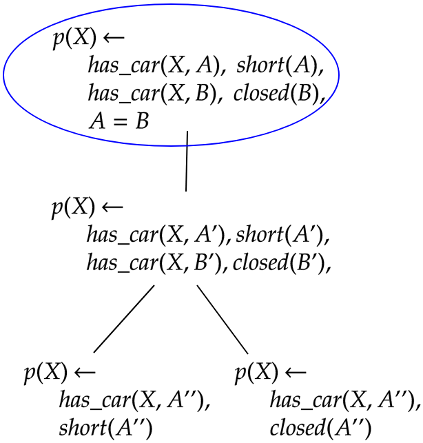So in both cases $l$ is in $\bigcup_{i=1}^{k}S_{i}$ . Hence $C\subseteq\bigcup_{i=1}^{k}S_{i}$ . ∎

Let $\mathrm{M}$ be a set of constrained mode-declarations, and $\mathrm{T}$ be a set of type definitions. Let $\mathrm{M}^{\prime}$ be $\mathrm{M}$ extended with an additional mode-declarations allowing body-literals of the form $+\gamma=+\gamma$ (that is, $\mathrm{M}^{\prime}$ allows equality between variables of the same type $\gamma$ , if this is not already allowed in $\mathrm{M}$ ); the definition of $=/2$ is provided by axioms of the equality logic. For more details see Appendix A. We note that if the ordered clause $\langle C\rangle$ is in ${\cal L}_{\mathrm{M},\mathrm{T}}$ , then $\langle C\rangle$ is in ${\cal L}_{\mathrm{M}^{\prime},\mathrm{T}}$ .

We define operators $\rho_{1},\rho_{2}$ as follows:

1.

Let $\langle C\rangle$ be in ${\cal L}_{\mathrm{M}^{\prime},\mathrm{T}}$ s.t. $\langle C\rangle:p(X)\leftarrow Body(X,{\mathbf{Y}})$ . Then $\rho_{1}(\langle C\rangle)$ = $\{$ $p(X)\leftarrow Body(X,{\mathbf{Y}}),Y_{1}=Y_{2}~|~$ $Y_{1},Y_{2}$ are output variables of the same type in $Body$ $\}$ ;
2.

Let $\langle{C}_{1}\rangle$ , $\langle{C}_{2}\rangle$ be in ${\cal L}_{\mathrm{M}^{\prime},\mathrm{T}}$ s.t. $\langle{C}_{1}\rangle:p(X)\leftarrow{Body}_{1}(X,{\mathbf{Y_{1}}})$ and $\langle{C}_{2}\rangle:(p(X)\leftarrow{Body}_{2}(X,{\mathbf{Y_{2}}})$ . Then $\rho_{2}(\langle{C}_{1}\rangle,\langle{C}_{2}\rangle)$ = $\{$ $p(X)\leftarrow{Body}_{1}(X,{\mathbf{Y}_{1}}),{Body}_{2}(X,{\mathbf{Y}_{2}})$ $\}$

These operators allows us to establish a link between the derivability of clauses in ${\cal L}_{\mathrm{M}^{\prime},\mathrm{T}}$ using $\{\rho_{1},\rho_{2}\}$ and clauses in ${\cal L}_{\mathrm{M},\mathrm{T}}$ .

Definition 8 (Derivation of Feature-Clauses)

Let $\mathrm{M}$ be a set of mode-declarations, and $\mathrm{M}^{\prime}$ be an extension of $\mathrm{M}$ as above. Let $\mathrm{T}$ be a set of type-definitions, and $\Omega\subseteq\{\rho_{1},\rho_{2}\}$ . Let ${\Phi}$ be a set of feature-clauses in ${\cal L}_{\mathrm{M}^{\prime},\mathrm{T}}$ . A sequence of feature-clauses $\langle C_{1}\rangle,\langle C_{2}\rangle,\dots,\langle C_{n}\rangle$ is said to be a derivation sequence of $\langle C_{n}\rangle$ from $\Phi$ using $\Omega$ iff each clause $\langle C_{i}\rangle$ in the sequence is either : (a) an instance of an element of $\Phi$ such that no variables other than $X$ occur earlier in this sequence; or (b) an element of the set $\rho_{1}(\langle C_{j}\rangle)$ ( $j<i$ ), if $\rho_{1}\in\Omega$ ; or (c) an element of the set $\rho_{2}(\langle C_{j}\rangle,\langle C_{k}\rangle)$ ( $j,k<i$ ), if $\rho_{2}\in\Omega$ . We will say $\langle C_{n}\rangle$ is derivable from $\Phi$ using $\Omega$ if there exists a derivation sequence of $\langle C_{n}\rangle$ from $\Phi$ using $\Omega$ .

Example 7

Let us assume the set of mode-declarations $\mathrm{M}$ contain the following:

	$\displaystyle\{~modeh(p(+train)),modeb(has\_car(+train,-car)),modeb(short(+car)),$
	$\displaystyle modeb(closed(+car)),modeb(smaller(+car,+car)~\},$

where $train$ and $car$ are type-names, with definitions in $\mathrm{T}$ . Here is a derivation sequence of

	$\displaystyle p(X)\leftarrow$	$\displaystyle~has\_car(X,U),has\_car(X,V),smaller(U,V),U=V,$
		$\displaystyle~has\_car(X,Y),short(Y),U=Y$

from

	$\displaystyle\{~p(X)$	$\displaystyle\leftarrow has\_car(X,Y),short(Y),$
	$\displaystyle p(X)$	$\displaystyle\leftarrow has\_car(X,U),has\_car(X,V),smaller(U,V)~\}$

using $\{\rho_{1},\rho_{2}\}$ .

1	$p(X)\leftarrow has\_car(X,U),has\_car(X,V),smaller(U,V)$	Given
2	$p(X)\leftarrow has\_car(X,U),has\_car(X,V),smaller(U,V),U=V$	$1,\rho_{1},U,V$
3	$p(X)\leftarrow has\_car(X,Y),short(Y)$	Given
4	$p(X)\leftarrow has\_car(X,U),has\_car(X,V),smaller(U,V),U=V,$
	$has\_car(X,Y),short(Y)$	$2,3,\rho_{2}$
5	$p(X)\leftarrow has\_car(X,U),has\_car(X,V),smaller(U,V),U=V,$
	$has\_car(X,Y),short(Y),U=Y$	$4,\rho_{1},U,Y$

It is useful to define the notion of a $\rho$ -derivation graph from a set of feature-clauses $\Phi$ .

Definition 9 ( $\rho$ -derivation graph given $\Phi$ )

Let $\gamma=(V,E,\phi)$ be a labelled DAG with vertices $V$ , edges $E$ and vertex-labelling function $\phi$ . Let $Pred(v)$ denote the set of immediate predecessors of any $v\in V$ . Let ${\cal F}_{\mathrm{M}}$ be a set of feature-clauses given modes $\mathrm{M}$ and $I\subseteq{\cal F}_{\mathrm{M}}$ . Let ${\Phi}$ be a set of feature-clauses in ${\cal L}_{\mathrm{M}^{\prime},\mathrm{T}}$ . Then $\gamma$ is a $\rho$ -derivation graph given $\Phi$ iff:

•

For each vertex $v_{i}\in V$ , $\phi(v_{i})=C_{i}$ , where $C_{i}\in{\cal F}_{\mathrm{M}}$ ;
•

$0\leq|Pred(v)|\leq 2$ for all $v\in V$ ;
•
For each $v\in V$ :
- –
  
  If $Pred(v)=\emptyset$ then $\phi(v)\in\Phi$ ;
- –
  
  If $Pred(v)=\{u\}$ then $\phi(v)\in\rho_{1}(\phi(u))$ ;
- –
  
  If $Pred(v)=\{u_{1},u_{2}\}$ then $\phi(v)\in\rho_{2}(\phi(u_{1}),\phi(u_{2}))$

Since we are only concerned with $\rho_{1},\rho_{2}$ in this paper, we will usually call this the derivation graph given $\Phi$ or even just the derivation graph, when $\Phi$ is understood.

Remark 4

We note that $\rho_{1}$ and $\rho_{2}$ preserve equivalence, in the following sense:

•

If $C^{\prime}\equiv C$ then $\rho_{1}(C)\equiv\rho_{1}(C^{\prime})$ ; and
•

If $C^{\prime}_{1}\equiv C_{1}$ and $C_{2}^{\prime}\equiv C_{2}$ then $\rho_{2}(C1,C2)\equiv\rho_{2}(C_{1}^{\prime},C_{2}^{\prime})$

Here, equivalence across sets has the usual conjunctive meaning. That is, for sets $A,B$ , $A\equiv B$ iff $\underset{x\in A}{\bigwedge}x~\equiv~\underset{y\in B}{\bigwedge}y$ . Two ordered clauses $\langle C_{1}\rangle$ and $\langle C_{2}\rangle$ are equivalent iff the $Set(\langle C_{1}\rangle)$ is equivalent to the $Set(\langle C_{2}\rangle)$ .

Definition 10 (Closure)

Let $\Phi$ be a set of feature-clauses and $\Omega\subseteq\{\rho_{1},\rho_{2}\}$ . We define the closure of $\Phi$ using $\Omega$ as the set of ordered clauses $\langle C\rangle$ which has a derivation sequence from $\Phi$ using $\Omega$ . We use $Closure_{\Omega}(\Phi)$ to denote the closure of $\Phi$ using $\Omega$ .

We will say $\theta$ is a type-consistent substitution if for every variable $U$ , the substitution $U/t\in\theta$ (that is, $\theta(U)=t$ ), then $U,t$ have the same type in $\mathrm{M}$ . It follows that if $\theta$ is a type-consistent substitution for variables in an ordered clause $\langle C\rangle$ in ${\cal L}_{\mathrm{M},\mathrm{T}}$ and $\theta(u)=\theta(v)$ for $u,v$ in $\langle C\rangle$ , then $u,v$ have the same type in $\mathrm{M}$ .

Lemma 2 (Derivation Lemma)

Given $\mathrm{M},\mathrm{M}^{\prime}$ and $\Omega=\{\rho_{1},\rho_{2}\}$ as before. Let $\langle C\rangle$ be an ordered clause in ${\cal L}_{\mathrm{M},\mathrm{T}}$ , with head $p(X)$ . Let $S$ be a set of ordered $\mathrm{M}$ -simple clauses in ${\cal L}_{\mathrm{M},\mathrm{T}}$ , with heads $p(X)$ and all other variables of clauses in $S$ standardised apart from each other and from $C$ . If there exists a substitution $\theta$ s.t. $Basis(\langle C\rangle)\subseteq S\theta$ then there exists an ordered clause $\langle C^{\prime}\rangle$ in ${\cal L}_{\mathrm{M}^{\prime},\mathrm{T}}$ such that $\langle C^{\prime}\rangle$ is equivalent to $\langle C\rangle$ and derivable from $S$ using $\Omega$ .

Proof

See Appendix C. ∎

Remark 5

Let $\langle C_{1}\rangle,\langle C_{2}\rangle,\ldots,\langle C_{n}\rangle$ be a derivation from a set of ordered clauses $S$ using $\{\rho_{1},\rho_{2}\}$ . Also, for any clause $\langle C_{i}\rangle$ in the derivation sequence, let $f_{i}$ denote the corresponding feature-function as defined in Section 2 using background knowledge $B$ . Let $a$ denote a data-instance. We note the following consequences for $1\leq i<j\leq n$ :

1.

$C_{i}$ subsumes $C_{j}$ ;⁵⁵ 5 Here subsumption is used in the sense described by Plotkin 1972. That is, representing clauses as sets of literals, clause $C$ subsumes clause $D$ iff there exists a substitution $\theta$ s.t. $C\theta\subseteq D$ .
2.

If $f_{i}(a)=0$ then $f_{j}(a)=0$ ;
3.

If $f_{j}(a)=1$ then $f_{i}(a)=1$ ; and
4.

If $\langle C_{i+1}\rangle\in\rho_{1}(\langle C_{i}\rangle)$ , $f_{i}(a)=1$ and $f_{i+1}(a)=0$ then there exists a clause $C_{i+1}^{\prime}$ s.t. $C_{i}\equiv C_{i+1}\vee C_{i+1}^{\prime}$ and $f_{B,C_{i+1}^{\prime}}(a)=1$

(1) follows straightforwardly since for any $\langle C_{i}\rangle$ , subsequent clauses in the derivation only result in the addition of literals (that is, $C_{i}\subset C_{j}$ for $i<j$ ). For (2), we note that since $C_{i}\subset C_{j}$ and both $C_{i},C_{j}$ have the same head literal ( $p(X)$ ) we can take $C_{i}=\forall(p(X)\vee l_{1}\vee\cdots l_{k})$ and $C_{j}=\forall(p(X)\vee l_{1}\vee\cdots l_{k}\vee l_{k+1}\vee\cdots l_{m})$ . If $f_{i}(a)=0$ then $B\cup C_{i}\not\models p(a)$ . That is, there exists some interpretation $I$ that is a model for $B\cup C_{i}$ s.t. $p(a)$ is false in $I$ . If $I$ is a model for $B\cup C_{i}$ then it is a model for $C_{i}$ . Further, if $I$ is a model for $C_{i}$ and $p(a)$ is false in $I$ then $I$ is a model for $\forall(l_{1}\vee\cdots l_{k})$ . But then $I$ is a model for $C_{j}=\forall(p(X)\vee l_{1}\vee\ldots l_{k}\vee l_{k+1}\vee\cdots l_{m})$ . Thus $I$ is a model for $B\cup C_{j}$ and not a model for $p(a)$ . That is, $B\cup C_{j}\not\models p(a)$ and $f_{j}(a)=0$ . (3) follows from the fact that if $C_{i}$ subsumes $C_{j}$ then $C_{i}\models C_{j}$ (Gottlob 1987). Therefore, if $B\cup C_{j}\models p(a)$ then $B\cup C_{i}\models p(a)$ . That is, if $f_{j}(a)=1$ then $f_{i}(a)=1$ . For (4), let $C_{i}:p(X)\leftarrow{Body}_{i}(X,{\mathbf{Y}})$ . Then $C_{i+1}:p(X)\leftarrow{Body}_{i}(X,{\mathbf{Y}}),Y_{i}=Y_{j}$ for $y_{i,j}\in{\mathbf{Y}}$ . Since $f_{i}(a)=1$ and $f_{i+1}(a)=0$ , it must be the case that $Y_{i}=Y_{j}$ does not hold for $x=a$ . Let $C_{i+1}^{\prime}:p(X)\leftarrow{Body}_{i}(X,{\mathbf{Y}}),Y_{i}\neq Y_{j}$ . It is evident that, $f_{B,C_{i+1}^{\prime}}(a)=1$ and $C_{i}\equiv C_{i+1}\vee C_{i+1}^{\prime}$ .

A specialised form of derivation results from the repeated use of $\rho_{2}$ first, followed by the repeated use of $\rho_{1}$ . We call this form of derivation a linear derivation. We describe this next (relevant proofs are in Appendix D).

Definition 11 (Linear Derivation of Feature-Clauses)

Let $\mathrm{M}$ be a set of mode-declarations, and $\mathrm{M}^{\prime}$ be an extension $\mathrm{M}$ as earlier. Let $\mathrm{T}$ be a set of type-definitions. Let ${\Phi}$ be a set of feature-clauses in ${\cal L}_{\mathrm{M}^{\prime},\mathrm{T}}$ and $\rho_{1},\rho_{2}$ be the operators defined earlier. A sequence of feature-clauses $\langle C_{1}\rangle,\langle C_{2}\rangle,\dots,\langle C_{n}\rangle$ is said to be a linear derivation sequence of $\langle C_{n}\rangle$ from $\Phi$ using $\{\rho_{1},\rho_{2}\}$ iff there exists $j$ such that $1\leq j\leq n$ and:

•
For $i\leq j$ :
- –
  
  Clause $\langle C_{i}\rangle$ in the sequence is either an element of $\Phi$ or an element of the set $\rho_{2}(\langle C_{i-1}\rangle,\langle C_{k}\rangle)$ where $\langle C_{k}\rangle\in\Phi$ and $k<i$ .
•
For $i>j$ :
- –
  
  Clause $\langle C_{i}\rangle$ is an element of the set $\rho_{1}(\langle C_{i-1}\rangle)$ .

We will say $\langle C_{j}\rangle$ is linearly derivable from $\Phi$ using $\{\rho_{2}\}$ ; and $C_{n}$ is linearly derivable from $\Phi$ using $\{\rho_{1},\rho_{2}\}$ .

Example 8

We continue Example 7. Below is a linear derivation sequence of

	$\displaystyle p(X)\leftarrow$	$\displaystyle~has\_car(X,U),has\_car(X,V),smaller(U,V),$
		$\displaystyle~has\_car(X,Y),short(Y),U=V,U=Y$

from

	$\displaystyle\{~p(X)$	$\displaystyle\leftarrow has\_car(X,Y),short(Y),$
	$\displaystyle p(X)$	$\displaystyle\leftarrow has\_car(X,U),has\_car(X,V),smaller(U,V)~\}$

using $\{\rho_{1},\rho_{2}\}$ .

1	$p(X)\leftarrow has\_car(X,U),has\_car(X,V),smaller(U,V)$	Given
2	$p(X)\leftarrow has\_car(X,Y),short(Y)$	Given
3	$p(X)\leftarrow has\_car(X,U),has\_car(X,V),smaller(U,V)$
	$has\_car(X,Y),short(Y)$	$1,\rho_{2}$
4	$p(X)\leftarrow has\_car(X,U),has\_car(X,V),smaller(U,V),$
	$has\_car(X,Y),short(Y),U=V$	$3,\rho_{1},U,V$
5	$p(X)\leftarrow has\_car(X,U),has\_car(X,V),smaller(U,V),$
	$has\_car(X,Y),short(Y),U=V,U=Y$	$4,\rho_{1},U,Y$

There is no way to derive the clause $p(X)\leftarrow has\_car(X,U),has\_car(X,V),$ $smaller(U,V),$ $U=V,has\_car(X,Y),short(Y),U=Y$ using linear derivation from the given set, but we can derive an equivalent clause $p(X)\leftarrow has\_car(X,U),has\_car(X,V),$ $smaller(U,V),$ $has\_car(X,Y)$ , $short(Y),U=V,U=Y$ using linear derivation. We would like to point out that the positions of equality literal $U=V$ in the first clause and the second clause are different.

Lemma 3 (Linear Derivation Lemma)

Given $M,M^{\prime}$ and a set of ordered clauses $\Phi$ . If an ordered clause $\langle C\rangle$ is derivable from $\Phi$ using $\{\rho_{1},\rho_{2}\}$ then there exists an equivalent ordered clause $\langle C^{\prime}\rangle$ and it is linearly derivable from $\Phi$ using $\{\rho_{1},\rho_{2}\}$ .

Proof

See Appendix D. ∎

Feature-clauses and their composition using the $\rho$ -operators provide the tools for the development of a particular kind of neural network that we describe next.

3 Compositional Relational Machines (CRMs)

Formally, a CRM is defined as follows:

Definition 12 (CRM)

A CRM is a 7-tuple $(V,I,O,E,\phi,\psi,h)$ where:

•

$V$ denotes a set of vertices;
•

$I\subseteq V$ is a set of “input” vertices;
•

$O\subseteq V$ is a set of “output” vertices;
•

$E\subseteq\{(v_{i},v_{j}):v_{i},v_{j}\in V,v_{i}\not\in O,v_{j}\not\in I\}$ ;
•

A vertex-labelling function $\phi:V\rightarrow{\cal F}_{\mathrm{M}}\times{\cal G}$ , where ${\cal F}_{\mathrm{M}}$ is the set of feature-clauses given a set of modes $\mathrm{M}$ ; and $\cal G$ denotes a set of activation functions.⁶⁶ 6 We assume activation functions in ${\cal G}$ are $\mathbb{R}\rightarrow\mathbb{R}$ . In this paper, we will further assume, if $v\in I$ then we restrict $\phi(v)=(\cdot,{\mathbf{1}})$ , where ${\mathbf{1}(\cdot)}$ = 1;
•

An edge labelling function $\psi:E\rightarrow\mathbb{R}$ , assigns some real-valued labels to edges in the graph; and
•

$h:{\mathbb{R}}^{|O|}\to{\mathbb{R}}^{n}$ is a computation function, for some fixed $n$

such that $(V,E,\phi^{\prime})$ is a derivation graph (Definition 9) given $\Phi$ where $\phi^{\prime}(v)=C$ if $\phi(v)=(C,\cdot)$ and $\Phi=\{\phi^{\prime}(v)~|~v\in I\}$ .

We note 2 important features of CRMs: (1) Each vertex has a feature-clause associated with it; and (2) Edges between vertices in a CRM are required to satisfy the constraints on edges imposed by a derivation graph. That is, the only edges allowed are those that result from $\rho_{1}$ or $\rho_{2}$ operations on the feature-clauses associated with the vertices.

3.1 CRMs as Explainable Neural Networks

We describe a use of CRMs as a form of neural network capable of generating logical explanations relevant to its prediction. The architecture of the neural network is inspired by Turing’s idea of unorganised machines (Turing 1948) (see Figure 1). Each “neuron” has 2 parts, implementing the vertex-label specification of a CRM’s node: (i) An arithmetic part that is concerned with the $g$ -function in the CRM’s vertex-label; and (ii) A logical part that acts as a switch, depending on the feature-clause associated with the CRM’s vertex-label. We call neurons in such a network “arithmetic-logic neurons” or ALNs for short.

Refer to caption — Figure 1: A neural network implementation of a CRM inspired by Turing’s gated neural networks (Turing 1948). A neuron $n_{i}$ corresponds to a vertex $v_{i}$ in the CRM, with vertex-label $\psi(v_{i})=(C_{i},g_{i})$ . In the figure, $n_{i}$ is connected to neurons $n_{j}$ and $n_{k}$ , implying $(v_{j},v_{i})$ and $(v_{k},v_{i})$ are in the edge-set of the CRM. $f_{i}$ (correctly $f_{C_{i},B})$ is the feature-function obtained from the feature-clause $C_{i}$ (see Section 2), and acts as a gate. For a data instance $a$ , $g_{i}(w_{ji}h_{j}(a)+w_{ki}h_{k}(a))$ passes through the gate if and only $f_{i}(a)=1$ . In general, $h_{i}(a)$ is thus $g_{i}(\sum_{k=Pred(n_{i})}w_{ki}h_{k}(a))$ or $0$ , where $Pred(n_{i})$ is the set of immediate predecessors of $n_{i}$ in the neural network.

In the rest of the paper, we will use “CRM” synonymously with this form of neural-network implementation. The 7-tuple defining a CRM $(V,I,O,E,\phi,\psi,h)$ corresponds to the following aspects of the neural implementation: (a) The structure of the network is defined by $V,I,O,E,$ and $\phi$ ; (b) The parameters of the network are defined by $\psi$ ; and (c) the computation of the network is defined by $h$ . We consider each of these in turn.

3.1.1 Structure Selection

Procedure 1is an enumerative procedure for obtaining a 5-tuple $(V,I,O,E,\phi$ ), given a set of feature-clauses $\Phi$ . For simplicity, the procedure assumes a single activation function $g$ .

Input: A set

\Phi

of feature-clauses

\{C_{1},C_{2},\ldots,C_{n}\}

with heads p(X) and all other variables are standardised apart from each other; an activation function g; and a bound

d

on the depth of composition

Output: A CRM structure

I=\{v_{1},v_{2},\ldots,v_{n}\}

; 1

V=I

; 2

E=\emptyset

; 3

for $i=1$ to $n$ do 4

\phi(v_{i})=(C_{i},\mathbf{1})

for $j=1$ to $d$ do 5

V_{j,1}=\{({C^{\prime}},v):v\in V,\phi(v)=(C,\cdot),C^{\prime}=\rho_{1}(C)\}

; 6

V_{j,2}=\{(C^{\prime},v_{1},v_{2}):v_{1},v_{2}\in V,\phi(v_{1})=(C_{1},\cdot),\phi(v_{2})=(C_{2},\cdot),C^{\prime}=\rho_{2}(C_{1},C_{2})\}

; 7

Let

V_{1}

be a set of new vertices

v

s.t. there exists

(C^{\prime},v^{\prime})\in V_{j,1}

and

\phi(v)=(C^{\prime},g)

; 8

Let

V_{2}

be a set of new vertices

v

s.t. there exists

(C^{\prime},v_{1},v_{2})\in V_{j,2}

and

\phi(v)=(C^{\prime},g)

; 9

Let

V^{\prime}=V_{1}\cup V_{2}

; 10

V=V\cup V^{\prime}

; 11

E=E\cup\{(v_{1},v):~(C,v_{1})\in V_{j,1},\phi(v)=(C,g)\}

\cup

\{(v_{1},v),(v_{2},v):~(C,v_{1},v_{2})\in V_{j,2},\phi(v)=(C,g)\}

; 12

O=\{v:v\in V,\nexists v^{\prime}~s.t.~(v,v^{\prime})\in E\}

; 13

return

(V,I,O,E,\phi)

Procedure 1 (ConstructCRM) Depth-bounded construction of a CRM’s structure

Procedure 1has an important practical difficulty:

•

We are interested in a class of CRMs that can be constructed using a set of $\mathrm{M}$ -simple feature-clauses $\{C_{1},\ldots,C_{n}\}$ . Now, it may be impractical to obtain all possible $\mathrm{M}$ -simple feature-clauses in a mode-language. Even if this were not the case, it may be impractical to derive all non-simple clauses in the manner shown in Procedure 1.

Procedure 2describes a randomised implementation to address this. The procedure also uses the result in the Linear Derivation Lemma (Lemma 3 in Section 2) to construct a CRM structure that first uses the $\rho_{2}$ operator, followed by the $\rho_{1}$ operator.

Input: A set

\Phi

of feature-clauses

\{C_{1},C_{2},\ldots,C_{n}\}

with heads p(X) and all other variables are standardised apart from each other; an activation function

g

; a sample size

s

; bounds

d_{\rho_{1}},d_{\rho_{2}}

on the depth of application of the

\rho_{1}

and

\rho_{2}

operators

Output: A CRM structure

I=\{v_{1},v_{2},\ldots,v_{n}\}

; 1

V_{0}=I

; 2

V=V_{0}

; 3

E=\emptyset

; 4

for $i=1$ to $n$ do 5

\phi(v_{i})=(C_{i},\mathbf{1})

; 6

for $j=1$ to $d_{\rho_{1}}+d_{\rho_{2}}$ do 7

V_{j}=\emptyset

; 8

E_{j}=\emptyset

; 9

if $j\leq d_{\rho_{2}}$ then 10

op=\rho_{2}

; 11

else 12

op=\rho_{1}

; 13

for $i=1$ to $s$ do 14

if $op=\rho_{2}$ then 15

Sample a vertex

v_{1}

from

I

using a uniform distribution and sample a vertex

v_{2}

from

V_{j-1}

using the uniform distribution; 16

Create a vertex

v^{\prime}

such that

\phi(v^{\prime})=(C^{\prime},g)

where

C^{\prime}=\rho_{2}(C_{1},C_{2})

\phi(v_{1})=(C_{1},g)

and

\phi(v_{2})=(C_{2},g)

; 17

V_{j}=V_{j}\cup\{v^{\prime}\}

; 18

E_{j}=E_{j}\cup\{(v_{1},v^{\prime}),(v_{2},v^{\prime})\}

; 19

else 20

Sample a vertex

v

from

V_{j-1}

using the uniform distribution; 21

Create a vertex

v^{\prime}

such that

\phi(v^{\prime})=(C^{\prime},g)

where

C^{\prime}=\rho_{1}(C)

and

\phi(v)=(C,g)

; 22

V_{j}=V_{j}\cup\{v^{\prime}\}

; 23

E_{j}=E_{j}\cup\{(v,v^{\prime})\}

; 24

V=V\cup V_{j}

; 25

E=E\cup E_{j}

; 26

O=\{v:v\in V,\nexists v^{\prime}~s.t.~(v,v^{\prime})\in E\}

; 27

return

(V,I,O,E,\phi)

; 28

Procedure 2 (RandomCRM) Randomised construction of a CRM structure, with linear derivation of feature-clauses.

In the rest of the paper, we will use the term Simple CRM to denote a CRM constructed by either Procedure 1 or Procedure 2 in which the input clauses $C_{1},C_{2},\ldots,C_{n}$ are $\mathrm{M}$ -simple feature-clauses.

3.1.2 Parameter Estimation

Procedure 2does not completely specify a CRM. Specifically, neither the edge-labelling $\psi$ nor $h$ are defined. We now describe a procedure that obtains a $\psi$ given the partial-specification returned by Procedure 2 and a pre-specified $h$ suitable for the usual task of using the neural network for function approximation. That is, given a partial specification of an unknown function $\delta:{\cal A}\to{\cal Y}$ in the form of sample data $D=\{(a_{i},y_{i})\}_{1}^{N}$ . We want the the neural network to construct an approximation $\hat{\delta}:{\cal A}\to{\cal Y}$ that is reasonably consistent with $D$ . In order to estimate the goodness of the approximation, we need to define a loss function, that computes the penalty of using $\hat{\delta}$ . We will take $\hat{\delta}$ to be synonymous with $h$ , the computation function of the CRM. Recall $h:{\mathbb{R}}^{|O|}\to\mathbb{R}^{n}$ for some fixed $n$ . In this paper, we will therefore take ${\cal Y}=\mathbb{R}^{n}$ and define $h$ in the usual manner adopted by neural networks, namely as a function of “local” computations performed at each of the $O$ vertices of the CRM.

Definition 13 (Local Computation in a CRM)

Let $(V,I,O,E,\phi,\psi)$ be a partially-specified CRM, where $O=\{o_{1},o_{2},\ldots,o_{k}\}$ . For each vertex $v_{i}\in V$ let $\phi(v_{i})=(C_{i},g_{i})$ and for each edge $(v_{i},v_{j})$ $\psi((v_{i},v_{j}))=w_{ij}$ . Let $f_{i}$ denote $f_{C_{i}}$ . For any $a\in{\cal A}$ we define $h_{i}:{\cal A}\rightarrow\mathbb{R}$ as follows:

h_{i}(a)=\left\{\begin{array}[]{ll}f_{i}(a)&\mbox{ if }v_{i}\in I\\ f_{i}(a)g_{i}\left(\sum_{(v_{j},v_{i})\in E}w_{ji}h_{j}(a)\right)&\mbox{ if }v_{i}\not\in I\\ \end{array}\right.

Then $\hat{\delta}(a)=h(h_{o_{1}}(a),\ldots,h_{o_{k}}(a))$ .

For a multi-class classification task, function $h$ computes the probability distribution over the classes, for example, a $\mathtt{softmax}$ function. Similarly, for a regression task, $h$ computes a real number, for example, a $\mathtt{linear}$ function.

Procedure 3estimates the parameters of the neural network using a standard weight-update procedure based on stochastic gradient descent (SGD) (Rumelhart et al. 1986; Goodfellow et al. 2016), given the structure obtained from Procedure 2, a pre-defined computation function $h$ , and a loss function $L$ .

Input: A CRM structure

\gamma=(V,I,O,E,\phi)

, a dataset

D=\{(a_{i},y_{i})\}_{1}^{N}

, where

a_{i}\in{\cal A}

and

y_{i}\in\mathbb{R}^{n}

, a computation function

h:{\mathbb{R}}^{|O|}\to\mathbb{R}^{n}

, a loss function

L:\mathbb{R}^{n}\times\mathbb{R}^{n}\to\mathbb{R}

Output: A CRM

Let

O=\{o_{1},\ldots,o_{k}\}

; 1

Initialise

\psi

; 2

while stopping criterion is not met do 3

Randomly draw an instance

(a_{i},y_{i})

from

D

; 4

Let

\hat{y_{i}}=h(h_{o_{1}}(a),\ldots,h_{o_{k}}(a))

(see Definition 13); 5

Error=L(y_{i},\hat{y_{i}})

; 6

Update

\psi

using SGD to minimise

Error

; 7

return

(V,I,O,E,\phi,\psi,h)

; 8

Procedure 3 (TrainCRM) Parameter estimation of a CRM, given its structure, using stochastic gradient descent (SGD). The training is done until some stopping criterion is reached, which refers to the condition when the number of training epochs reaches some pre-specified maximum value.

3.1.3 Predictions and Explanations

We denote the prediction of a CRM $\gamma=(V,I,O,E,\phi,\psi,h)$ by $\hat{\delta}(a)=h(h_{o_{1}}(a),\ldots,h_{o_{k}}(a))$ , where $O=\{o_{1},\ldots,o_{k}\}$ and the $h_{o_{i}}$ are as defined in Definition 13.

The association of feature-clauses with every vertex of the CRM allows us to construct “explanations” for predictions. For this we introduce the notion of ancestral graph of a vertex and explanation graph of an output vertex in a CRM.

Definition 14 (Ancestral Graph of a Vertex)

Let $\gamma=(V,I,O,E,\phi,\psi,h)$ be a CRM. The set of ancestors of a vertex $v\in V$ in $\gamma$ , denoted by $Ancestors(v,\gamma)$ , is defined as follows:

Ancestors(v,\gamma)=\left\{\begin{matrix}\{v\}&\mathrm{if}~v\in I\\ \bigcup_{(u,v)\in E}Ancestors(u,\gamma)\cup\{v\}&\mathrm{otherwise}\end{matrix}\right.

The ancestral graph of a vertex $v$ in $\gamma$ is $(V^{\prime},E^{\prime})$ where $V^{\prime}=Ancestors(v,\gamma)$ and $E^{\prime}=\{(u^{\prime},u^{\prime\prime}):u^{\prime},u^{\prime\prime}\in V^{\prime},(u^{\prime},v^{\prime\prime})$ in $E\}$ .

Definition 15 (Explanation Graph)

Let $\gamma=(V,I,O,E,\phi,\psi,h)$ be a CRM, and $a\in{\cal A}$ be a data instance. Let $O=\{o_{1},\ldots,o_{k}\}$ and let $\hat{\delta}(a)=h(h_{o_{1}}(a),\ldots,h_{o_{k}}(a))$ be the prediction of the CRM for $a$ . For $o_{i}\in O$ , let $C_{i}$ be the feature-clause associated with $o_{i}$ (that is, $\phi(o_{i})=(C_{i},\cdot)$ ). Let $f_{i}$ be the corresponding feature-function (as defined in Section 2), and $(V^{\prime},E^{\prime})$ be an ancestral graph of $o_{i}$ in $\gamma$ . Then the explanation graph of $a$ from vertex $o_{i}$ , denoted by ${Explain}_{\gamma,o_{i}}(a)$ , is as follows:

Explain_{\gamma,o_{i}}(a)=\left\{\begin{matrix}(V^{\prime},E^{\prime},\phi^{\prime})&\mathrm{if}~f_{i}(a)=1\\ \emptyset&\mathrm{otherwise}\end{matrix}\right.

where $\phi^{\prime}:V^{\prime}\rightarrow{\cal F}_{\mathrm{M}}$ is a vertex-labelling function. $\phi^{\prime}(v)=C\theta_{a}$ , where $\theta_{a}$ the substitution $\{X/a\}$ for the variable $X$ in the head literal and $\phi(v)=(C,\cdot)$ .

Remark 6

${Explain}_{\gamma,o_{i}}(a)$ consists of a (labelled) tree of feature-clauses extracted from the derivation graph of feature-clauses. The root of the tree is the feature-clause at $o_{i}$ and sub-trees contain simpler feature-clauses. If the CRM is a Simple CRM, then the leaves of the explanation-tree are $\mathrm{M}$ -simple feature-clauses.

Example 9

In the Trains problem, suppose the data instance is the train shown on the left below. The explanation graph, associated with an output vertex of the CRM is shown on the right.



(Train $t1$ )		(additionally requires the substitution $\{X/t1\}$ to be applied)

By definition, we know that the feature-function value associated with $p(t1)\leftarrow has\_car(t1,A),$ $short(A),$ $has\_car(t1,B),$ $closed(B)$ has the value $1$ . Also, we know that feature-function values with all other clauses in the explanation will also be $1$ .

The notion of an explanation graph from a vertex extends naturally to the explanation graph from a set of vertices which we do not describe here. It will be useful in what follows to introduce the notion of a feature-clause being “contained in an explanation graph”.

Definition 16 (Feature-clause Containment)

Let $\gamma$ be a CRM, $o$ be an output vertex of $\gamma$ , Let $a$ be a data instance, Let ${Explain}_{\gamma,o}(a)=(V,E,\alpha)$ , and $F_{\gamma,o}(a)=\{\alpha(v)~|~v\in V\}$ be the set of feature-clauses in the explanation graph. We will say a feature-clause $C$ is contained in ${Explain}_{\gamma,o}(a)$ , or $C\sqsubseteq{Explain}_{\gamma,o}(a)$ iff there exists $C^{\prime}\in F_{\gamma,o}(a)$ s.t. $C\theta_{a}\equiv C^{\prime}$ (where $\theta_{a}=\{X/a\}$ , is a substitution for the variable $X$ in the head of $C$ ).

(This naturally extends to the containment of a set of clauses.)

Example 10

The feature-clause $C:$ $p(X)\leftarrow$ $has\_car(X,Y),$ $short(X),$ $closed(X)$ is contained in the explanation graph shown for train $t_{1}$ in Figure 6 because:

•
$F_{\gamma,o}(t_{1})$ $=$ $\{C_{1},C_{2},C_{3},C_{4}\}$ where:
1. $C_{1}:$ $p(t_{1})\leftarrow(has\_car(t_{1},A),$ $short(A),$ $has\_car(t_{1},B),$ $closed(B),$ $A=B)$ ;
2. $C_{2}:$ $p(t_{1})\leftarrow(has\_car(t_{1},A^{\prime}),$ $short(A^{\prime}),$ $has\_car(t_{1},B^{\prime}),$ $closed(B^{\prime}))$ ;
3. $C_{3}:$ $p(t_{1})\leftarrow(has\_car(t_{1},A^{\prime\prime}),$ $short(A^{\prime\prime}))$ ; and
4. $C_{4}:$ $p(t_{1})\leftarrow(has\_car(t_{1},A^{\prime\prime}),$ $closed(A^{\prime\prime}))$
•

With $\theta_{a}=\{X/t_{1}\}$ , $C\theta_{a}$ = $(p(t_{1})\leftarrow(has\_car(t_{1},A),$ $short(A),$ $closed(A))$ ; and
•

$C\theta_{a}\equiv C_{1}$

Explanatory Fidelity

Explanatory fidelity refers to how closely the CRM’s explanation matches the “true explanation”. Of course, in practice, explanatory fidelity will be a purely notional concept, since the true explanation will not be known beforehand. However it is useful for us to calibrate the CRM’s explanatory performance when it is used for problems where true explanations are known (the synthetic problems considered in experiments below are in this category).

For a prediction $\hat{\delta}(h_{o_{i}}(a),\ldots,h_{o_{k}}(a))$ by a CRM, suppose we have a relevance ordering over the output vertices $o_{1},\ldots,o_{k}$ . Let $o^{*}$ be the most relevant vertex in this ordering. Then we will call the explanation graph from $o^{*}$ as the most-relevant explanation graph for $a$ given the CRM.⁷⁷ 7 In implementation terms, one way to obtain such a relevance ordering over output vertices of the CRM is to use the $h_{i}(\cdot)$ values for vertices in $O$ to select a vertex $o^{*}$ that has the highest magnitude (this is the same as selecting the best vertex after one iteration of the layer-wise relevance propagation, or LRP (Binder et al. 2016), procedure).

For a classification task, we use clause containment and the most-relevant explanation graph to arrive at a notion of explanatory fidelity of a CRM to a set of feature-clauses ${\cal T}_{c}$ that are known to be ‘acceptable’ feature-clauses for class $c$ (if no such acceptable clauses exist for class $c$ , then ${\cal T}_{c}=\emptyset$ ). Let $\gamma$ be a CRM used to predict the class-labels for a set of data-instances. For any instance $a$ , let $o^{*}$ denote the most relevant output vertex of the CRM. We will say that a data instance $a$ is consistently explained iff: (i) the CRM predicts that $a$ has the class-label $c$ ; and (ii) there exists a $C\in{\cal T}_{c}$ s.t. $C\sqsubseteq{Explain}_{\gamma,o^{*}}(a)$ ; and (iii) for $c^{\prime}\neq c$ , there does not exist $C^{\prime}\in{\cal T}_{c^{\prime}}$ s.t. $C^{\prime}\sqsubseteq{Explain}_{\gamma,o^{*}}(a)$ .

Given a set of data-instances $E$ , let $CE$ denote the set of instances in $E$ explained consistently and $IE$ denote the set of instances in $E$ not explained consistently. Then the explanatory fidelity of the CRM (correctly, this is only definable w.r.t. the ${\cal T}_{c}$ ’s) is taken to be $\frac{|CE|}{|CE|+|IE|}$ , provided $(|CE|+|IE|)\neq 0$ (and undefined otherwise).

3.2 CRMs as Explanation Machines

CRMs can be used as ‘explanation machines’ for black-box predictors that do not intrinsically include an explanatory component. The approach, sometimes called post hoc explanation generation, is shown in Figure 2.

To assess the utility of using the CRM in this manner, we will change the usual assessment of predictive accuracy to one of ‘predictive fidelity’, which refers to how closely the CRM matches the prediction of the target model.

4 Empirical Evaluation of CRMs as Explanation Machines

4.1 Aims

We consider two kinds of experiments with Simple CRMs:

Synthetic data.: Using tasks for which both target-model predictions and acceptable feature-clauses are available, we intend to investigate the hypothesis that: (a) Simple CRMs can construct models with high predictive fidelity to the target’s prediction; and (b) Simple CRMs have high explanatory fidelity to the set of acceptable feature-clauses.
Real data.: Using real-world datasets, for which we have predictions from a state-of-the-art black-box target model, we investigate the hypothesis that Simple CRMs can construct models with high predictive fidelity to the target’s prediction. We also provide illustrative examples of using the CRM to provide explanations for the predictions.

We clarify what is meant by ‘acceptable feature-clauses’ for the synthetic data in Section 4.3. For real data, the target-model is the state-of-the-art (SOTA, which in this case is a graph-based neural network). That is, the CRM is being used here to match the SOTA’s predictions (and not the ‘true value’), and to provide proxy explanations. No acceptable feature-clauses are known for classes in the real data.⁸⁸ 8 The CRM can of course be used to predict the true value directly. We will comment on this later, but that is not the primary goal of the experiment here.

4.2 Materials

4.2.1 Data and Background Knowledge

Synthetic Data.

We use two well-known synthetic datasets. The first dataset is the “Trains” problem of discriminating between eastbound (class = $+$ ) and westbound trains (class = $-$ ) (Michalski 1980). The original data consists only of 10 instances (5 in each class). We generate a dataset of 1000 instances with a class-disitribution of approximately 50% $+$ and 50% $-$ , using the data generator (Michie et al. 1994). We use 700 instances as training data and 300 instances as test-data. The second dataset consists of the task of discriminating between illegal (class = $+$ ) and legal (class = $-$ ) chess positions in the King-Rook-King endgame (Bain 1994; Michie 1976). The class-distribution is approximately 33% $+$ and 67% $-$ . We use 10000 instances of board-positions as training data and 10000 instances as test-data. Examples of $+$ instances are showed pictorially in Figure 3.

Real Data.

Our real data consists of 10 datasets obtained from the NCI⁹⁹ 9 The National Cancer Institute (https://www.cancer.gov/). Each dataset represents extensive drug evaluation with the concentration parameter GI50, which is the concentration that results in 50% growth inhibition of cancer cells (Marx et al. 2003). A summary of the dataset is presented in Figure 4. Each relational data-instance in a dataset describes a chemical compound (molecule) with atom-bond representation: a set of bond facts. The background knowledge consists of logic programs defining almost $100$ relations for various functional groups (such as amide, amine, ether, etc.) and various ring structures (such as aromatic, non-aromatic etc.). There are also higher-level domain-relations that determine presence of connected, fused structures. Some more details on the background knowledge can be seen in these recent studies: (Dash et al. 2021; Dash et al. 2022).

# of	Avg. # of	Avg. # of	Avg. # of	% of
datasets	instances	atoms per instance	bonds per instance	positives
10	3018	24	51	50–75
				Avg. $=57$

Figure 4: Summary of the NCI-50 datasets (Total no. of instances is approx. 30,200). The graph neural network predictor described in (Dash et al. 2021) is taken as the target model. No acceptable feature-clauses are known for these tasks.

4.2.2 Algorithms and Machines

We use the ILP system Aleph (Srinivasan 2001) for constructing the feature-clauses. The CRMs are implemented using PyTorch (Paszke et al. 2019). The parameter learning of CRMs has been done with the autograd engine available within PyTorch for the implementation of backpropagation. Our implementation of Layerwise-Relevance Propagation (LRP) is based on (Bach et al. 2015; Binder et al. 2016).

The CRM implementation and all our experiments are conducted on a workstation running with Ubuntu (Linux) operating system, 64GB main-memory, and a CPU running with 12 Intel Xeon processors.

4.3 Method

The experiments are in two parts: an investigation on synthetic data to examine the predictive performance and explanatory fidelity of CRMs; and an investigation on real data, to compare the predictive performance of CRMs against state-of-the-art deep networks. Some examples of explanations are also provided for the explanations generated by a CRM on real data. We describe the method used for each part in turn.

4.3.1 Experiments with Synthetic Data

For both synthetic datasets, we have access to symbolic descriptions of the true concepts involved. The ‘target model’ in each case is taken to be equivalent to a classifier that labels instances consistent with the corresponding true concept. This allows us to judge the fidelity of explanations generated. The method used in each case is straightforward:

For each problem:
1. (a)
  
  Construct the dataset $D$ of instances labelled by the target model;
2. (b)
  
  Generate a subset of $\mathrm{M}$ -simple feature-clauses in the mode-language for the problem;
3. (c)
  
  Randomly split $D$ into training and test samples;
4. (d)
  
  Construct a CRM using Procedure 2 with the $\mathrm{M}$ -simple features. The weights for the CRM are obtained using the training data and the SGD-based weight-update steps described in Procedure 3 (see below for additional details);
5. (e)
  
  Obtain an estimate of the predictive and the explanatory fidelity of the CRM using the test data (again, see below for details).

The following additional details are relevant to the method just described:

•

For both datasets, the composition depth of CRMs is at most 3. Also, the mode-declarations for Chess allow the occurrence of equalities in $\mathrm{M}$ -simple features (see Appendix F), additional compositions using $\rho_{1}$ are not used in this problem;
•

We use the rectified linear ( $\mathtt{relu}$ ) activation function for the local computation in the neurons of the internal (hidden) layers of the CRMs.
•

We use Adam optimiser (Kingma and Ba 2015) to minimise the training cross-entropy loss between the true classes and the predicted classes by the network;
•

We provide as input feature-clauses only a subset of all possible $\mathrm{M}$ -simple feature-clauses. The subset is constrained by the following: (i) At most 2 body literals; (ii) Minimum support of at least 10 instances¹⁰¹⁰ 10 In principle, increasing the number of input clauses will increase the size (width and breadth) of the CRM (measured by the number of layers and neurons in each layer of the CRM). Furthermore, since complex features are more specific than the features represented by simple clauses, the coverage of the complex features (that is, instances for which the features have the value 1) will usually be lower than those of simple clauses. Thus, if we restrict complex features to those having a positive coverage of at least $p$ , simple features will have also have a coverage of at least $p$ . Thus, simple features with a lower positive coverage will not be part of any connection in the CRM, and therefore need not appear in the inputs.; and (iii) Minimum precision of at least 0.5. All subsequent feature-clauses obtained by composition are also required to satisfy the same support and precision constraints. The learning rate for the Adam optimiser is set to $0.001$ while keeping other hyperparameters to their defaults within PyTorch;
•

The number of training epochs is set to $5$ for the Trains dataset and $10$ for the Chess dataset;
•

Both synthetic problems are binary classification tasks. We call the classes $+$ and $-$ for convenience. Predictive fidelity is estimated in the usual manner, namely as the proportion of correctly predicted test-instances;

•

Explanatory fidelity is estimated as described in Section 3.1.3. For this, we need to pre-define sets of feature-clauses that are acceptable in explanations. For the synthetic datasets, we are able to identify sets of acceptable feature-clauses from the literature: These feature-clauses are obtained from a target model that is known to be complete and correct (see (Michie et al. 1994) for the target model for Trains and (Bain 1994) for Chess). The acceptable clauses in ${\cal T}_{+}$ are as follows:

Problem	Acceptable Feature Clause
Trains	$p(X)\leftarrow has\_car(X,Y),short(X),closed(X)$
Chess	$p((A,B,C,D,C,E))\leftarrow true$
	$p((A,B,C,D,E,D))\leftarrow true$
	$p((A,B,A,B,C,D))\leftarrow true$
	$p((A,B,C,D,E,F))\leftarrow adj(A,E),adj(B,F)$

In Trains, the feature clauses apply to descriptions of trains. For Chess these are descriptions of the board in an endgame. The board is a 6-tuple that denotes the file and rank of the position of the White King, White Rook and Black King, respectively. In all cases ${\cal T}_{-}=\emptyset$ . Explanatory fidelity will be estimated by checking clause-containment of the feature-clauses above in the explanation graph for the most-relevant output vertex of the CRM (see Section 3.1.3);

•

The acceptable feature-clause for the Trains is a direct rewrite of the function used to generate the labels. For Chess, the (set of) feature-clauses are direct rewrites of an approximate symbolic description taken from (Srinivasan et al. 1992). These approximate description isn’t identical to the correct description, but is very closely related to it (the approximation differ from the correct description only in about 40 of 10,000 cases). For our purposes therefore, high explanatory fidelity, w.r.t. the set of feature-clauses shown, will taken to be sufficient; and
•

We provide a baseline comparison for predictive fidelity against a ‘majority class’ predictor. A baseline comparison is also provided for explanatory fidelity against random selection of a feature-clause from the set of feature-clauses associated with the output vertices of the CRM that have a feature-function value of 1 for the data instance being predicted.

4.3.2 Experiments with Real Data

For the real-world datasets, the current state-of-the-art predictions are from a Graph Neural Network (GNN) constructed using the background knowledge described earlier (Dash et al. 2022). However, the GNN model constitutes a black-box model, since it does not produce any explanations for its predictions. We investigate equipping this black-box model with CRM model for explanation. The method is as follows:

For each problem:
1. (a)
  
  Construct the dataset $D$ consisting of problem instances and their predictions of the target model;
2. (b)
  
  Generate a subset of $\mathrm{M}$ -simple feature-clauses in the mode-language for the problem. The restrictions used for synthetic data are used to constrain the subset;
3. (c)
  
  Construct a CRM using Procedure 2 with the $\mathrm{M}$ -simple features and the dataset $D$ . The weights for the CRM are obtained using the training data used by the state-of-the-art methods and the SGD-based weight-update procedure; and
4. (d)
  
  Obtain the predictive fidelity of the CRM model to the predictions of the target model.

The following additional details are relevant:

•

As with the synthetic data, the compositional depth for the CRMs is set to $3$ . Again, we do not use $\rho_{1}$ operations, since the mode-declarations allow equalities. The constraints on input feature-clauses is the same as those used for synthetic data;¹¹¹¹ 11 Our choice for the compositional depth of $3$ is also loosely-based on our previous work on Deep Relational Machines (DRMs: (Dash et al. 2018)). However, we note that a depth higher than $3$ will increase the complexity of a CRM (due to increase in number of layers and neurons), which might result in better predictive performance of a CRM. We expect that in practice the depth bound will be treated as a hyperparameter and subject to the usual forms of hyperparameter optimisation.
•

The CRM implementation is the same as the one used for synthetic data. We perform a grid-search of the learning rate for the Adam optimiser using the parameter grid: $\{0.01,0.001,0.005,0.0001\}$ . The total number of training epochs is $10$ , with early-stopping mechanism (Prechelt 1998) with a patience period of $3$ ;
•

As with the synthetic data, we provide a baseline comparison against the ‘majority class’ predictor;
•

Unlike the synthetic data, no pre-defined set of acceptable feature-clauses exists, and therefore no estimate of explanatory fidelity is possible. Correspondingly, there is no baseline provided either.

4.4 Results

Figure 5tabulates the results used to compute estimates of predictive and explanatory fidelity on synthetic and real data. The main details in these tabulations are these: (a) For the synthetic data, Simple CRMs models able to match the target’s prediction perfectly (predictive fidelity of 1.0); (b) The high explanatory fidelity values show that for instances labelled $+$ , the maximal explanation for the most-relevant vertex contains at least 1 clause from the set of acceptable feature-clauses; and for instances labelled $-$ , the maximal explanation of the most relevant vertex does not contain any clauses from the target theory; and (c) On the real datasets predictive fidelity of CRMs is reasonably high: suggesting that about 81% of the time, the CRM’s prediction will match that of the state-of-the-art model.

Dataset	Fidelity
	CRM		Baseline
	Pred.	Expl.	Pred.	Expl.
Trains	1.0	1.0	0.5	0.4
Chess	1.0	0.9	0.7	0.7

(a) Synthetic data

Dataset	Pred. Fidelity
	CRM	Baseline
786_0	0.77	0.53
A498	0.79	0.59
A549_ATCC	0.85	0.63
ACHN	0.73	0.58
BT_549	0.78	0.51
CAKI_1	0.81	0.69
CCRF_CEM	0.82	0.68
COLO_205	0.77	0.53
DLD_1	0.90	1.00
DMS_114	0.89	0.91
Avg.	0.81 (0.05)	0.66 (0.17)

(b) Real data

Figure 5: Estimates of fidelity for Simple CRMs on the synthetic datasets and real datasets. Explanatory fidelity is assessable on synthetic data since we have access to the “correct” explanation. Baseline for prediction is the majority class predictor. For explanations, Baseline refers to random selection of a feature-clause from the set of feature-clauses associated with the output vertices of the CRM with function value

1

for the data instance being predicted by the majority class predictor.

We now turn to examine the results in greater detail.

4.4.1 Predictive Fidelity

Although we obtain perfect predictive fidelity to the target model on synthetic data, fidelity on the real datasets clearly has room for improvement. Improvements in fidelity are possible simply by considering ensembles of CRMs, obtained simply due to the sampling variation arising in Step (c) (refer Section 4.3.2). Below, we tabulate changes in predictive fidelity on 1 of the real-world problems (786_0), using a sample consisting of upto 3 CRMs. With multiple CRMs, for a data-instance to be correctly predicted it is sufficient for any one of the CRMs to predict the same class as the target-model. Recall the primary purpose of the CRM is to explain the target-model’s prediction in terms of its feature-clauses. Any CRM that matches the target-model’s prediction can be used to explain the prediction. More on this under “Explanation” below.

No. of	Predictive
CRMs	Fidelity
1	0.75
2	0.83
3	0.85

4.4.2 Explanatory Fidelity

For the synthetic datasets we show below in Figure 6 a representative $+$ instance (shown pictorially for ease of understanding), along with the predictions of both target and the CRM. The last column shows an acceptable feature-clause along with a stylised English translation. In both instances, an equivalent form of the acceptable feature-clause is contained in the CRM’s explanation graph.

For the Chess data, the CRM’s explanatory fidelity is less than $1$ . This means that there are instances for which the CRM’s explanation graph does not contain an acceptable feature-clause. We discover 19 different kinds of ‘buggy’ explanations are found by the CRM: a full listing is in Appendix F. Here we provide illustrative instances of two kinds of errors: those that are close to the correct explanation; and those that are an artifact of the specific data instance being explained (see Figure 7). Besides these, in many cases, we find explanation errors arise from the fact that definitions in background knowledge of file and rank adjacency hold when ranks and files are the same (that is, if $A$ and $B$ are ranks (or files) and $A=B$ , then $adj(A,B)$ is true).¹²¹² 12 M. Bain, the author of the background definitions, confirms that this is the intended meaning of the $adj/2$ predicate for this problem (personal communication). In many instances inconsistent explanations result from feature-clauses contain literals that use equality instead of adjacency (that is, the CRM’s explanation contains $A=E$ , rather than $adj(A,E)$ : see Section F.2 in Appendix F). However, even accounting for this, the CRM’s explanations can be more specific than the correct explanation; and in some cases, incorrect (an example of each is shown in Figure 7).

What about explanations on real data? At this point, we do not have any independent source of acceptable feature-clauses for this data. We nevertheless show a representative example of the explanation for a test-instance (see Figure 8).

We close this examination by drawing the reader’s attention to an important aspect of a CRM’s explanation. The feature-clauses are defined in terms of relations provided as prior knowledge. This makes them potentially intelligible to a person familiar with the meanings of these relations. This makes it easier–in principle at least–to perform a human-based assessment of the feature-clauses in the explanation graph (this is apparent from the ‘debugging’ of explanations that we have been to accomplish with the Chess data).

4.4.3 Additional Results: CRMs as Prediction Machines

The tabulations of fidelity and the subsequent assessments above provide a measure of confidence in the use of CRMs as explanation machines. But it is evident that CRMs can be used as ‘white-box’ predictors in their own right. We provide an indicative comparison of a CRM predictor against the state-of-the-art predictors (for the real-data, the prediction is by majority-vote from an ensemble of 3 CRMs):

Dataset	Predictive accuracy
	CRM	GNN	DRM (500)	CILP++	Baseline
786_0	0.66 (0.01)	0.69 (0.01)	0.69 (0.01)	0.67 (0.01)	0.55 (0.01)
A498	0.67 (0.01)	0.72 (0.01)	0.70 (0.01)	0.66 (0.01)	0.52 (0.01)
A549_ATCC	0.64 (0.01)	0.67 (0.01)	0.70 (0.01)	0.60 (0.01)	0.51 (0.01)
ACHN	0.64 (0.01)	0.70 (0.01)	0.70 (0.01)	0.64 (0.01)	0.51 (0.01)
BT_549	0.66 (0.01)	0.68 (0.01)	0.70 (0.01)	0.65 (0.01)	0.53 (0.01)
CAKI_1	0.63 (0.01)	0.68 (0.01)	0.66 (0.01)	0.64 (0.01)	0.54 (0.01)
CCRF_CEM	0.65 (0.01)	0.71 (0.01)	0.71 (0.01)	0.68 (0.01)	0.63 (0.01)
COLO_205	0.60 (0.01)	0.69 (0.01)	0.67 (0.01)	0.66 (0.01)	0.56 (0.01)
DLD_1	0.69 (0.02)	0.69 (0.02)	0.70 (0.02)	0.72 (0.02)	0.69 (0.02)
DMS_114	0.68 (0.02)	0.74 (0.02)	0.75 (0.02)	0.75 (0.02)	0.76 (0.02)

Figure 9: Predictive performance comparison of an ensemble of

3

Simple CRMs against some leading black-box predictors. The numbers are estimates of predictive accuracy obtained on test data. The number in parentheses is the estimated standard deviation. The techniques being compared are: GNN, the graph-based neural network approach described in (Dash et al. 2022); DRM (

500

), is a form of MLP called a Deep Relational Machine that has, as input, Boolean feature-vectors resulting from a stochastic selection of

500

relational features (Dash et al. 2019); and CILP++, an MLP that has input Boolean feature-vectors resulting from an exhaustive feature construction technique called Bottom-Clause Propositionalisation (França et al. 2014). Baseline is the majority class predictor.

The results in Figure 9 indicate that Simple CRMs perform approximately as well as CILP++ (França et al. 2014), but are worse than either the GNN (Dash et al. 2022) or DRM (Dash et al. 2019). However, Figure 9 are best treated as preliminary. Variations in CRMs arise in Procedure 2 purely due to sampling, of course. However, the CRM obtained is also affected by the following: (1) The subset constraints on support and precision all feature-clauses in the CRM; (2) bounds on the depth of compositions $\rho_{2}$ followed by $\rho_{1}$ operators; (3) The number of feature-clauses drawn in each layer of the CRM. Additional variation can arise from the initialisation of weights for the SGD-based estimation of parameters. This suggests that substantially more experimentation is needed to see if the predictive performance of Simple CRMs can be improved. We note also that the DRM uses substantially more complex features than the Simple CRM, and that CILP++ constructs substantially more features than the Simple CRM (anywhere between 30,000 to 50,000 compared to about 330 $\mathrm{M}$ -simple features for the CRMs). Of course none of GNN, DRM or CILP++ have any intrinsic mechanism of associating explanations with their prediction.

5 Related Work

We note first that $\rho_{1}$ and $\rho_{2}$ are closely related to the notion of refinement operators which have been studied extensively in ILP, in the context of the search through a hypothesis space (see (Tamaddoni-Nezhad and Muggleton 2009; Nienhuys-Cheng et al. 1997)). Our motivation in this paper is, however, in the use of these operators to derive relational features. Consequently, we describe connections to related work in 3 categories: conceptual work on relational features; implementation and applied work on propositionalisation in ILP; and work on explainable deep networks.

On the conceptual understanding of relational features, perhaps the most relevant single summary is in (Saha et al. 2012). There the authors identify several feature-classes, based on somewhat similar notions of source- and sink-literals. The relationship between the different classes in that paper is shown in Figure 10(a). The relationship to these sets of the class of $\mathrm{M}$ -simple feature-clauses, denoted here as $F_{\mathrm{M}}$ , is shown in Figure 10(b) (see Appendix E for more details).

Simple clauses in (McCreath 1999) and the corresponding set of features in $F_{s}$ are restricted to determinate predicate-definitions.¹³¹³ 13 Informally, a determinate predicate is one whose definition encodes a function. That is, for a given set of values for input arguments, there is exactly one set of values for output arguments. Results in (McCreath 1999) show that features from $F_{s}$ can be used to derive the subset of feature-clauses in $F_{d}$ that only contain determinate predicate-definitions. There is no such restriction imposed on $F_{\mathrm{M}}$ and all clauses in $F_{d}$ (and therefore all other classes shown) can be derived using some composition of $\rho_{1}$ and $\rho_{2}$ . No corresponding operators or completeness results are known for $F_{r}$ .

Relational features have been shown to be an extremely effective form of learning with relational objects (Kramer et al. 2001; Lavrač et al. 2021). Methods that construct and use relational features, guided by some form of mode-declarations can be found in (Srinivasan and King 1999; Lavrač et al. 2002; Ramakrishnan et al. 2007; Joshi et al. 2008; Specia et al. 2009; Faruquie et al. 2012; Saha et al. 2012; França et al. 2014; Vig et al. 2017; Dash et al. 2018). Of these, the features in Lavrač et al. 2002 are from the feature class $F_{r}$ . There are no reports on the class of features used in the other reports, although the procedures for obtaining the features suggest that they are not restricted to any specific sub-class (that is, they are simply from $F_{d}$ ). Given our results on derivation of features in $F_{d}$ from features in $F_{\mathrm{M}}$ , and the class-inclusions shown, we would expect at least some features in a super-class would require additional composition operations to those in a sub-class. In terms of a CRM structure, we would expect features in $F_{i}$ , for example, would usually be associated with vertices at a greater depth than those in $F_{r}$ . Empirical results tabulated for some statistical learners in (Saha et al. 2012) suggest that relational features from the class $F_{i}$ were most useful for statistical learners. If this empirical trend continues to hold, then we would expect the performance of CRMs to improve as depth increases (and features in $F_{i}$ are derived), and then to flatten or decrease (as features in $F_{d}\setminus F_{i}$ are derived).

The development and application of CRMs is most closely related to the area of self-explainable deep neural networks (Alvarez Melis and Jaakkola 2018; Angelov and Soares 2020; Ras et al. 2022). The structure of the CRM enforces a meaning to each node in the network, and in turn, we have shown here how to extract one form of explanation from these meanings. A different kind of neural network, also with meanings associated nodes is described in (Sourek et al. 2018). Those networks are also explainable, although not in the manner described here. In (Srinivasan et al. 2019), a symbolic proxy-explainer is constructed using ILP for a form of multi-layer perceptron (MLP) that uses as input values of relational features. The features there drawn from the class $F_{d}$ , and the explanations are logical rules constructed by ILP using the feature-definitions provided to the MLP. There are at least two important differences to the explanations constructed there and the ones obtained with a CRM: (i) The rules constructed in (Srinivasan et al. 2019) effectively only perform the $\rho_{2}$ operation on relational features. This can result in a form of incompleteness: some features in $F_{d}$ cannot be represented by the rules, unless they are already included as input to the MLP; and (ii) The structuring of explanations in (Srinivasan et al. 2019) requires relevance information: here, the structuring is from usual functional (de)composition.

6 Conclusion

It has been long-understood in machine learning that the choice of representation can make a significant difference to the performance and efficiency of a machine learning technique. Representation is also clearly of relevance when we are interested in constructing human-understandable explanations for predictions made by the machine learning technique. A form of machine learning that has paid particular attention to issues of representation is the area of Inductive Logic Programming (ILP). A form of representation that has been of special interest in ILP is that of a relational feature. These are Boolean-valued functions defined over objects, using definitions of relations provided as prior- or background knowledge. The use of relational features forms the basis of an extremely effective form of ILP called propositionalisation. This obtains a Boolean-vector description of objects in the data, using the definition of the relational features and the background knowledge. Despite the obvious successes of propositionalisation, surprising little is known, conceptually, about the space of relational features. In this paper, we have sought to address this by examining relational features within a mode-language $\mathrm{M}$ , introduced in ILP within the setting of mode-directed inverse entailment (Muggleton 1995). Within a mode-language, we identify the notion of $\mathrm{M}$ -simple relational features, and two operations $\rho_{1}$ and $\rho_{2}$ that allows us to compose progressively more complex relational feature in the mode-language. In the first half of the paper, we show that $\rho_{1}$ and $\rho_{2}$ are sufficient to derive all relational features within a mode-language $\mathrm{M}$ . This generalises a previous result due to McCreath and Sharma 1998b, which was restricted to determinate definitions for predicates in the background knowledge, albeit starting from a different definition of simple features to that work.

In the second half of the paper, we use the notion of $\mathrm{M}$ -simple features and the composition operators $\rho_{1}$ and $\rho_{2}$ to construct a kind of deep neural network called a Compositional Relational Machine, or CRM. A special aspect of CRMs is that we are able to associate a relational feature with each node in the network. The structure of the CRM allows us to identify further how the feature at the node progressively decomposes into simpler features, until an underlying set of $\mathrm{M}$ -simple features are reached. This corresponds well to the intuitive notion of a structured explanation, that is composed of increasingly simpler components. We show how this aspect of CRMs allows them to be used as “explanation machines” for black-box models. Our results on synthetic and real-data suggest that CRMs can reproduce target-predictions with high fidelity; and the explanations constructed on synthetic data suggest that CRM’s explanatory structure usually also contains an acceptable explanation.

We have not explored the power of CRMs as “white-box” predictors in their own right, but early results suggest that it may be possible to obtain CRMs with good predictive accuracy. Although still significantly lower than the state-of-the-art, we believe this can change. We have also not explored other forms of CRMs, both simpler and more elaborate. For example, the identification of $\mathrm{M}$ -simple features and their subsequent compositions using the $\rho$ -operators suggests an even simpler CRM structures than that used here. It is possible for example, simply to obtain all possible compositions to some depth, and use a Winnow-like parameter estimation (Littlestone 1988) to obtain a self-explainable linear model. Equally, more complex CRMs are possible by incorporating weights on the $\mathrm{M}$ -simple features (this could be implemented simply by changing the activation function at the input nodes of the network). Taking this one step further, it is possible to associate weights with all the relational features, which will allow the use of the inference machinery of probabilistic logic programs (De Raedt et al. 2019). We think an investigation of these other kinds of compositional relational machines would contribute positively to the growing body of work in human-intelligible machine learning.

Acknowledgements.

AS is a Visiting Professor at Macquarie University, Sydney and a Visiting Professorial Fellow at UNSW, Sydney. He is also the Class of 1981 Chair Professor at BITS Pilani, Goa and a Research Associate at TCS Research. AS and TD would like to thank Lovekesh Vig and Gautam Shroff at TCS Research for interesting discussions on explainable neural networks; and Michael Bain at UNSW for discussions on the use of ILP for constructing symbolic explanations.

Declaration

Funding: Not applicable.
Conflicts of interest: Not applicable.
Ethics approval: Not applicable.
Consent to participate: Not applicable.
Consent for publication: Not applicable.
Data and code availability: All data and codes used in our research can be found at: https://github.com/tirtharajdash/CRM.
Authors’ contributions: AS and AB conceived and worked on the conceptual parts related to simple features and their composition, and the specification of CRMs. TD conceived and worked on the implementation of CRMs as gated neural networks. AS and TD conceived and worked on the application of CRMs to synthetic- and real-data. DS was involved in some parts of the implementation of CRMs.

Appendix A Logic Terminology

In this section we cover only terminology used in the paper, and further confined largely to logic programming. For additional background and further terminology see (Lloyd 2012; Chang and Lee 2014; Nilsson 1991; Muggleton and de Raedt 1994). The summary below is adapted from (Srinivasan et al. 2019).

A language of first order logic programs has a vocabulary of constants, variables, function symbols, predicate symbols, logical implication ‘ $\leftarrow$ ’, and punctuation symbols. A function or predicate can have a number of arguments known as terms. Terms are defined recursively. A constant symbol (or simply “constant”) is a term. A variable symbol (or simply “variable”) is a term. If $f$ is an $m$ -ary function symbol, and $t_{1},\ldots,t_{m}$ are terms, then the function $f(t_{1},\ldots,t_{m})$ is a term. A term is said to be ground if it contains no variables.

We use the convention used in logic programming when writing clauses. Thus, predicate, function and constant symbols are written as a lower-case letter followed by a string of lower- or upper-case letters, digits or underscores (‘_’). Variables are written similarly, except that the first letter must be upper-case. This is different to the usual logical notation, where predicate-symbols start with upper-case, and variables start with lower-case: however the logic programming syntax is useful for the implementation of CRMs. Usually, predicate symbols will be denoted by symbols like $p,q,r$ , etc., and symbols like $X,Y,Z$ to denote variables. If $p$ is an $n$ -ary predicate symbol, and $t_{1},\ldots,t_{n}$ are terms, then the predicate $p(t_{1},\ldots,t_{n})$ is an atom. Predicates with the same predicate symbol but different arities are distinguished by the notation $p/n$ where $p$ is a predicate of arity $n$ .

A literal is either an atom or the negation of an atom. If a literal is an atom it is referred to as a positive literal, otherwise it is a negative literal. A clause is a disjunction of the form $A_{1}\vee\ldots\vee A_{i}\vee\neg A_{i+1}\vee\ldots\vee\neg A_{k}$ , where each $A_{j}$ is an atom. Alternatively, such a clause may be represented as an implication (or “rule”) $A_{1},\ldots,A_{i}\leftarrow A_{i+1},\ldots,A_{k}$ . A definite clause $A_{1}\leftarrow A_{2},\ldots,A_{k}$ has exactly one positive literal, called the head of the clause, with the literals $A_{2},\ldots,A_{k}$ known as the body of the clause. A definite clause with a single literal is called a unit clause, and a clause with at most one positive literal is called a Horn clause. A set of Horn clauses is referred to as a logic program. It is often useful to represent a clause as a set of literals.

A substitution $\theta$ is a finite set $\{v_{1}/t_{1},\ldots,v_{n}/t_{n}\}$ mapping a set of $n$ distinct variables $v_{i}$ , $1\leq i\leq n$ , to terms $t_{j}$ , $1\leq j\leq n$ such that no term is identical to any of the variables. A substitution containing only ground terms is a ground substitution. For substitution $\theta$ and clause $C$ the expression $C\theta$ denotes the clause where every occurrence $C$ of a variable from $\theta$ is replaced by the corresponding term from $\theta$ . If $\theta$ is a ground substitution then $C\theta$ is called a ground clause. Since a clause is a set, for two clauses $C$ , $D$ , the set inclusion $C\theta\subseteq D$ is a partial order called subsumption, usually written $C$ $\theta$ -subsumes $D$ and denoted by $C\preceq D$ . For a set of clauses $S$ and the subsumption ordering $\preceq$ , we have that for every pair of clauses $C,D\in S$ , there is a least upper bound and greatest lower bound, called, respectively, the least general generalisation (lgg) and most general unifier (mgu) of $C$ and $D$ , which are unique up to variable renaming. The subsumption partial ordering on clauses enables the definition of a lattice, called the subsumption lattice.

We assume the logic contains axioms allowing for inference using the equality predicate $=/2$ . This includes axioms for reflexivity ( $\forall x(x=x)$ ), and substitution ( $\forall x~(\phi(x)\wedge(x=y)\longrightarrow\phi(y))$ ).

Appendix B Mode Language

We borrow some of the following definitions from (Dash et al. 2022). The definition of $\lambda\mu$ sequence is simplified as we are dealing only with feature clauses here and all other definitions are same as in (Dash et al. 2022).

Definition 17 (Term Place-Numbering)

Let $\pi=\langle i_{1},\ldots,i_{k}\rangle$ be a sequence of natural numbers. We say that a term $\tau$ is in place-number $\pi$ of a literal $\lambda$ iff: (1) $\pi\neq\langle\rangle$ ; and (2) $\tau$ is the term at place-number $\langle i_{2},\ldots,i_{k}\rangle$ in the term at the $i_{1}^{\mathrm{th}}$ argument of $\lambda$ . $\tau$ is at a place-number $\pi$ in term $\tau^{\prime}$ : (1) if $\pi=\langle\rangle$ then $\tau=\tau^{\prime}$ ; and (2) if $\pi=\langle i_{1},\ldots,i_{k}\rangle$ then $\tau^{\prime}$ is a term of the form $f(t_{1},\ldots,t_{m})$ , $i_{1}\leq m$ and $\tau$ is in place-number $\langle i_{2},\ldots,i_{k}\rangle$ in $t_{i_{1}}$ .

Definition 18 (Type-Names and Type-Definitions)

Let $\Gamma$ be a set of types and $\mathrm{T}$ be a set of ground-terms. For $\gamma\in\Gamma$ we define a set of ground-terms $T_{\gamma}$ = $\{\tau_{1},\tau_{2},\ldots\}$ , where $\tau_{i}\in\mathrm{T}$ . We will say a ground-term $\tau_{i}$ is of type $\gamma$ if $\tau_{i}\in T_{\gamma}$ , and denote by $T_{\Gamma}$ the set $\{T_{\gamma}:\gamma\in\Gamma\}$ . $T_{\Gamma}$ will be called a set of type-definitions.

Definition 19 (Mode-Declaration)

1.

Let $\Gamma$ be a set of type names. A mode-term is defined recursively as one of: (i) $+\gamma$ , $-\gamma$ or $\#\gamma$ for some $\gamma\in\Gamma$ ; or (ii) $\phi({mt}_{1}^{\prime},{mt}_{2}^{\prime},\ldots,{mt}_{j}^{\prime})$ , where $\phi$ is a function symbol of arity $j$ , and the ${mt}_{k}^{\prime}$ s are mode-terms.
2.

A mode-declaration $\mu$ is of the form $modeh(\lambda^{\prime})$ or $modeb(\lambda^{\prime})$ . Here $\lambda^{\prime}$ is a ground-literal of the form $p({mt}_{1},{mt}_{2},\ldots,{mt}_{n})$ where $p$ is a predicate name with arity $n$ , and the ${mt}_{i}$ are mode-terms. We will say $\mu$ is a $modeh$ -declaration (resp. $modeb$ -declaration) for the predicate-symbol $p/n$ . In general there can be several $modeh$ or $modeb$ -declarations for a predicate-symbol $p/n$ . We will use $ModeLit(\mu)$ to denote $\lambda^{\prime}$ .
3.

$\mu$ is said to be a mode-declaration for a literal $\lambda$ iff $\lambda$ and $ModeLit(\mu)$ have the same predicate symbol and arity.

Let $\tau$ be the term at place-number $\pi$ in $\mu$ , We define

ModeType(\mu,\pi)=\left\{\begin{matrix}(+,\gamma)&~\mathrm{if}~\tau=+\gamma\\ (-,\gamma)&~\mathrm{if}~\tau=-\gamma\\ (\#,\gamma)&~\mathrm{if}~\tau=\#\gamma\\ unknown&~\mathrm{otherwise}\end{matrix}\right.

5.

If $\mu$ is a mode-declaration for literal $\lambda$ , $ModeType(\mu,\pi)$ = $(+,\gamma)$ for some place-number $\pi$ , $\tau$ is the term at place $\pi$ in $\lambda$ , then we will say $\tau$ is an input-term of type $\gamma$ in $\lambda$ given $\mu$ (or simply $\tau$ is an input-term of type $\gamma$ ). Similarly we define output-terms and constant-terms.

We will also say that mode $\mu$ contains an input argument of type $\gamma$ if there exists some term-place $\pi$ of $\mu$ s.t. $ModeType(\mu,\pi)=(+,\gamma)$ . Similarly for output arguments.

Definition 20 ( $\lambda\mu$ -Sequence)

Assume a set of type-definitions $T_{\Gamma}$ , modes $\mathrm{M}$ . Let $\langle C\rangle=\langle l_{1},\neg l_{2},l_{3}\ldots,\neg l_{k}\rangle$ be an ordered clause. Then $\langle(\lambda_{1},\mu_{1}),(\lambda_{2},\mu_{2}),\dots,(\lambda_{k},\mu_{k})\rangle$ is said to be a $\lambda\mu$ -sequence for $\langle C\rangle$ iff it satisfies the following constraints:

Match.: (i) $\lambda_{i}=l_{i}$ ; (ii) For $j=1,\dots,k$ , $\mu_{j}$ is a mode-declaration for $\lambda_{j}$ s.t. $\mu_{j}=modeh(\cdot)$ ( $j=1$ ) and $\mu_{j}=modeb(\cdot)$ ( $j>1$ ).
Terms.: (i) If $\tau$ is an input- or output-term in $\lambda_{j}$ given $\mu_{j}$ , then $\tau$ is a variable in $\lambda_{j}$ ; (ii) Otherwise if $\tau$ is a constant-term in $\lambda_{j}$ given $\mu_{j}$ then $\tau$ is a ground term.
Types.: (i) If there is a variable $v$ in both $\lambda_{i}$ , $\lambda_{j}$ then the type of $v$ in $\lambda_{i}$ given $\mu_{i}$ is the same as the type of $v$ in $\lambda_{j}$ given $\mu_{j}$ ; (ii) If $\tau$ is a constant-term in $\lambda_{i}$ and the type of $\tau$ in $\lambda_{i}$ given $\mu_{i}$ is $\gamma$ , then $\tau\in T_{\gamma}$ .
Ordering.: (i) If $\tau$ is an input-term in $\lambda_{j}$ given $\mu_{j}$ and $j>1$ then there is an input-term $\tau$ in $\lambda_{1}$ given $\mu_{1}$ ; or there is an output-term $\tau$ in $\lambda_{i}$ ( $m<i<j$ ) given $\mu_{i}$ . (ii) If $\tau$ is an output-term in $\lambda_{1}$ given $\mu_{1}$ , then $\tau$ is an output-term of some $\lambda_{i}$ ( $1<i\leq k$ ) given $\mu_{i}$ .

Definition 21 (Mode-Language)

Assume a set of type-definitions $\mathrm{T}$ and modes $\mathrm{M}$ . The mode-language ${\cal L}_{\mathrm{M},\mathrm{T}}$ is $\{\langle C\rangle:$ either $C=\emptyset$ or there exists a $\lambda\mu$ -sequence for $\langle C\rangle\}$ .

Appendix C Proof of the Derivation Lemma

Lemma 2 (Derivation Lemma)

Proof

We prove this in 3 parts:

1.
We first show: if $Basis(\langle C\rangle)\subseteq S\theta$ , then $\theta$ is a type-consistent substitution for clauses in $S$ .
- Let $Basis(\langle C\rangle)$ = $\{\langle C_{1}\rangle,\ldots,\langle C_{k}\rangle\}$ and $S^{\prime}=\{\langle S_{1}\rangle,\ldots,\langle S_{k}\rangle\}\subseteq S$ . Without loss of generality, let $\langle S_{i}\rangle\theta=\langle C_{i}\rangle$ . Let $\theta=\{Y_{1}/t_{1},Y_{2}/t_{2},\ldots,Y_{n}/t_{n}\}$ where the $Y_{i}$ are variables in $S$ and the $t_{i}$ are terms in $Basis(\langle C\rangle)$ . In general, the $t_{i}$ ’s are variables, constants, or functional terms. Let $t_{j}$ be a constant. Suppose clause $S_{i}$ has the variable $Y_{j}$ in some location in $S_{i}$ and clause $C_{i}$ has the constant $t_{j}$ in the corresponding location. Since both $S_{i}$ and $C_{i}$ are in ${\cal L}_{\mathrm{M},\mathrm{T}}$ , this is only possible if there are multiple mode-declarations for the corresponding literals in $S_{i}$ and $C_{i}$ . But constraint MC2 (in Section 2.2) ensures that there is exactly one mode-declaration for any literal. Therefore $t_{i}$ cannot be a constant. Reasoning similarly, $t_{i}$ cannot be a functional term. Therefore $t_{i}$ has to be a variable in $C_{i}$ . Since $Y_{j}$ and $t_{j}$ are in the same locations for some literal $l$ in $S_{i}$ and $C_{i}$ , and there is only one mode-declaration for $l$ in $\mathrm{M}$ , it follows that the types of $Y_{j}$ and $t_{j}$ must be the same.
2.
If there exists a type-consistent substitution $\theta$ for clauses in $S$ , then there is an ordered clause $\langle C^{\prime\prime}\rangle$ in ${Closure}_{\{\rho_{2}\}}(S)$ s.t. $C^{\prime\prime}\theta\equiv C$ .
- Let us fix an ordering among the simple clauses in $S$ : $S_{1},\ldots,S_{k}$ , where $S_{i}=p(X)\leftarrow Body_{i}(X,\mathbf{Y_{i}})$ . Let us define a sequence of ordered clauses $\langle C_{1}\rangle$ , $\langle C_{2}\rangle$ , $\dots$ , $\langle C_{k}\rangle$ where $\langle C_{1}\rangle$ is $\langle S_{1}\rangle$ , and $\langle C_{i}\rangle$ is in $\rho_{2}(\langle C_{i-1}\rangle,\langle S_{i}\rangle)$ for $i=2$ to $k$ . It is easy to see that the above sequence is a derivation sequence of $\langle C_{k}\rangle$ from $\{\langle S_{1}\rangle,\langle S_{2}\rangle,\dots,\langle S_{k}\rangle\}$ using $\{\rho_{2}\}$ . That is, $\langle C_{k}\rangle$ is in ${Closure}_{\{\rho_{2}\}}(S)$ . $\langle C_{k}\rangle$ is of the form $p(X)\leftarrow Body_{1}(X,\mathbf{Y_{1}}),Body_{2}(X,\mathbf{Y_{2}}),$ $\dots,Body_{k}(X,\mathbf{Y_{k}})$ . That is $C_{k}=\bigcup_{i=1}^{k}S_{i}$ . Since $S\theta=Basis(\langle C\rangle)$ , then $C=\bigcup_{i=1}^{k}S_{i}\theta$ . Let $\langle C^{\prime\prime}\rangle$ = $\langle C_{k}\rangle$ That is, $C^{\prime\prime}\theta=C$ . Hence $C^{\prime\prime}\theta\equiv C$ . Also, since $\theta$ is a type-consistent substitution for clauses $S_{i}\in S$ , and $C^{\prime\prime}=\bigcup_{i}S_{i}$ , $\theta$ is a type-consistent substitution for $C^{\prime\prime}$ .
3.
From above $\langle C^{\prime\prime}\rangle$ and $\theta$ , we construct an ordered clause $\langle C^{\prime}\rangle$ in ${\cal L}_{\mathrm{M}^{\prime},\mathrm{T}}$ s.t. $\langle C^{\prime}\rangle$ is in $Closure_{\{\rho_{1}\}}(\{\langle C^{\prime\prime}\rangle\})$ and $C^{\prime\prime}\theta\equiv C^{\prime}$ .
- Let $\langle C^{\prime\prime}\rangle$ $=(p(X)\leftarrow Body(X,{\mathbf{Y}}))$ , and $\theta=\{Y_{1}/Y_{1}^{\prime},\ldots,Y_{l}/Y_{l}^{\prime}\}$ . It is easy to see that $\theta$ induces an equivalence relation on the variables in $C^{\prime\prime}$ . Variables $Y_{i}$ and $Y_{j}$ are in the same equivalence class if both variables map to the same variable $Y_{m}^{\prime}$ . For each equivalence class $[U]$ , we earmark one element in the class as representative of the class. This element is denoted by $rep([U])$ . Let $C^{\prime\prime}$ be $p(X)\leftarrow Body(X,{\mathbf{Y}})$ . Let us fix an order among the variables occurring in $\langle C^{\prime\prime}\rangle$ : $Y_{1},Y_{2},\dots,Y_{l}$ . Consider the following sequence of ordered clauses $\langle C_{0}\rangle,\langle C_{1}\rangle,\dots,\langle C_{l}\rangle$ where $\langle C_{0}\rangle=\langle C^{\prime\prime}\rangle$ , and $\langle C_{i}\rangle=p(X)\leftarrow Body(X,\mathbf{Y}),Y_{1}=rep([Y_{1}])$ , $Y_{2}=rep([Y_{2}]),\dots,Y_{l}=rep([Y_{l}])$ . The above sequence is a derivation of $\langle C_{l}\rangle$ from $\langle C^{\prime\prime}\rangle$ using only $\rho_{1}$ . That is $\langle C_{l}\rangle$ is in ${Closure}_{\{\rho_{1}\}}(\{\langle C^{\prime\prime}\rangle\})$ . Let $\langle C^{\prime}\rangle$ be $\langle C_{l}\rangle$ and it is of the form $p(X)\leftarrow Body(X,{\mathbf{Y}}),Y_{1}=rep([Y_{1}]),\ldots,Y_{l}=rep([Y_{l}])$ . It is easy to see that $\langle C^{\prime}\rangle\in{\cal L}_{\mathrm{M}^{\prime},\mathrm{T}}$ . We now show $C^{\prime\prime}\theta\equiv C^{\prime}$ . Let $\theta=\theta^{\prime\prime}\circ\theta^{\prime}$ , where $\theta^{\prime\prime}=\{Y_{1}/rep([Y_{1}]),\ldots,Y_{l}/rep([Y_{l}]\}$ and $\theta^{\prime}=\{rep([Y_{1}])/Y_{1}^{\prime},\ldots,$ $rep([Y_{l}])/Y_{l}^{\prime}\}$ .¹⁴¹⁴ 14 Correctly, $\theta^{\prime}$ and $\theta^{\prime\prime}$ have to be functions. It is evident that $\theta^{\prime\prime}$ is a function, since each variable maps to the representative of its equivalence class. We argue informally that $\theta^{\prime}$ is a function as follows. If $Y_{i}$ and $Y_{j}$ are in the same equivalence class, then $rep([Y_{i}])$ and $rep([Y_{j}])$ are the same variables. But according to our $\theta^{\prime}$ , they are mapped to $Y_{i}^{\prime}$ and $Y_{j}^{\prime}$ . One might think $\theta^{\prime}$ is not a function. But the variables in the same equivalence class are mapped to same variable. So $Y_{i}^{\prime}$ is the same as $Y_{j}^{\prime}$ and hence $\theta^{\prime}$ is a function. The variables $rep([Y_{i}])$ are in $S$ and the variables $Y_{i}^{\prime}$ are in $C$ . Since the variables in $S$ are standardised apart from the variables in $C$ , $\theta^{\prime}$ is a renaming substitution. Therefore $C^{\prime\prime}\theta^{\prime}\equiv C^{\prime\prime}$ . Therefore $C^{\prime\prime}\theta$ $\equiv$ $C^{\prime\prime}\theta^{\prime\prime}$ . By the substitution axiom in the equality logic $C^{\prime\prime}\theta^{\prime\prime}$ $\equiv$ $C^{\prime}$ . Therefore $C^{\prime\prime}\theta\equiv C^{\prime}$ .

From (1)–(3) above, the result follows. ∎

Appendix D Properties of Derivations using $\rho_{1},\rho_{2}$

Lemma 4 (Reordering Lemma)

Given $M,M^{\prime}$ and a set of ordered clauses $\Phi$ . If an ordered clause $\langle C\rangle$ is derivable from $\Phi$ using $\{\rho_{1},\rho_{2}\}$ then: (a) there is a derivation for $\langle C_{j}\rangle$ from $\Phi$ using $\{\rho_{2}\}$ ; (b) there is a derivation for $\langle C_{k}\rangle$ from $\{\langle C_{j}\rangle\}$ using $\{\rho_{1}\}$ ; and (c) $\langle C\rangle$ is equivalent to $\langle C_{k}\rangle$ .

Proof

Let us assume there is a derivation $\tau$ for $\langle C\rangle$ from $\Phi$ using $\{\rho_{1},\rho_{2}\}$ . There exists an ordered clause $\langle C_{k}\rangle$ equivalent to $\langle C\rangle=p(X)\leftarrow l_{1},l_{2},\dots,l_{j},l_{j+1},l_{j+2},\dots,l_{k}$ such that

•

the sequence of literals $l_{1},\dots,l_{j}$ can be split into $Body(X,Y_{1}),\dots,Body(X,Y_{m})$ such that $p(X)\leftarrow Body(X,Y_{i})\in\Phi$ for each $i=1,\dots,m$ , and
•

$l_{j+1},\dots,l_{k}$ are equality predicates introduced using $\rho_{1}$ operator in the derivation $\tau$ . Let $\langle C_{j}\rangle$ be $p(X)\leftarrow Body(X,Y_{1}),\dots,Body(X,Y_{m})$ .

It is easy to see that there is derivation $\tau_{1}$ for $\langle C_{j}\rangle$ from $\Phi$ using $\rho_{2}$ operator. Now we can apply $\rho_{1}$ operator on $\langle C_{j}\rangle$ repeatedly to derive $\langle C_{k}\rangle$ . ∎

Lemma 5

Given $M,M^{\prime}$ and a set of ordered clauses $\Phi$ . If an ordered clause $\langle C\rangle$ is derivable from $\Phi$ using $\{\rho_{2}\}$ then it is linearly derivable from $\Phi$ using $\{\rho_{2}\}$ .

Proof

Let us assume that $\langle C\rangle$ is derivable from $\Phi$ using $\{\rho_{2}\}$ . Hence there exists a derivation sequence $\xi$ of ordered clauses $\langle C_{1}\rangle,\langle C_{2}\rangle,\dots,\langle C_{n}\rangle$ from $\Phi$ using $\{\rho_{2}\}$ and $\langle C_{n}\rangle=\langle C\rangle$ . Now we use mathematical induction to prove that for each $1\leq i\leq n$ , there exists a linear derivation of $\langle C_{i}\rangle$ from $\Phi$ using $\{\rho_{2}\}$ .

Base step:: Case $n=1$ is easy as $\langle C_{1}\rangle$ should be in $\Phi$ and hence there is a linear derivation for $\langle C_{1}\rangle$ from $\Phi$ using $\{\rho_{2}\}$ .
Induction step:: We assume there exists a linear derivation for $\langle C_{i}\rangle$ from $\Phi$ using $\{\rho_{2}\}$ for each $i<j$ (induction hypothesis) and prove that there exists a linear derivation for $\langle C_{j}\rangle$ . The clause $\langle C_{j}\rangle$ occurs in the derivation sequence $\xi$ . There are two cases to be considered: it is in $\Phi$ or it is in $\rho_{2}(\langle C_{l}\rangle,\langle C_{m}\rangle)$ where $l,m<j$ . If $\langle C_{j}\rangle$ is in $\Phi$ , there exists a linear derivation sequence for $\langle C_{j}\rangle$ from $\Phi$ (just the one step derivation containing itself). Now we prove the claim for the second case. Since $l,m<j$ , by induction hypothesis, there exist linear derivation sequences $\xi_{l}$ for $\langle C_{l}\rangle$ and $\xi_{m}$ for $\langle C_{m}\rangle$ from $\Phi$ using $\{\rho_{2}\}$ . Let $\langle C_{1}^{\prime}\rangle,\langle C_{2}^{\prime}\rangle,\dots,\langle C_{k}^{\prime}\rangle$ be the clauses in $\Phi$ and occurring in $\xi_{m}$ . Now consider the following sequence $\xi_{j}$ containing $\xi_{l}$ , $\langle C_{1}^{\prime}\rangle$ , $\langle C_{1}^{\prime\prime}\rangle$ , $\langle C_{2}^{\prime}\rangle$ , $\langle C_{2}^{\prime\prime}\rangle$ ,…, $\langle C_{k}^{\prime}\rangle$ , $\langle C_{k}^{\prime\prime}\rangle$ where $\langle C_{1}^{\prime\prime}\rangle\in\rho_{2}(\langle C_{l}\rangle,\langle C_{1}^{\prime}\rangle)$ and $\langle C_{a}^{\prime\prime}\rangle\in\rho_{2}(\langle C_{a-1}^{\prime\prime}\rangle,\langle C_{a}^{\prime}\rangle)$ for $a=2$ to $k$ . It is easy to see that $\xi_{j}$ is a linear derivation sequence for $\langle C_{j}\rangle$ from $\Phi$ using $\rho_{2}$ . Hence there exists a linear derivation sequence for $\langle C_{n}\rangle$ from $\Phi$ using $\{\rho_{2}\}$ .

∎

Now the linear derivation lemma (re-stated below) can be easily proved by combining the above two lemmas.

Lemma 3 (Linear Derivation Lemma)

Appendix E Relationship of $\mathrm{M}$ -Simple Feature-Clauses to Known Feature Classes

We note the following about the sets of feature-clauses in Figure 10(b) and the set $F_{\mathrm{M}}$ of $\mathrm{M}$ -simple feature clauses:

The set $F_{d}$ .

This is identical to the set of ordered feature-clauses in the mode-language $\mathrm{M}$ ;

The set $F_{i}$ .

This set is defined based on a given mode language $M$ (but without constraints MC–MC3). An ordered feature clause $\langle C\rangle$ is in $F_{i}$ iff the number of connected components after removing the source vertex (corresponding to the head literal) from the clause dependency graph of $\langle C\rangle$ is exactly one. Since the clause dependency graph of a clause in $F_{\mathrm{M}}$ has exactly one sink literal and any vertex in that graph has a path to that sink vertex (Remark 2). So the number of connected components after removing the source vertex is one. Hence $F_{\mathrm{M}}\subseteq F_{i}$ . It is easy to see that $F_{i}\not\subseteq F_{\mathrm{M}}$ (see the counterexample given for $F_{s}\subseteq F_{\mathrm{M}}$ ).

The set $F_{s}$ .

This set is defined based on the class of simple clauses identified by McCreath 1999 who proposed simple clauses. We note:

1.

Feature-clause definitions in $F_{s}$ do not refer to a mode-language. The clause dependency-graph is constructed using a procedure described in (McCreath 1999), and is based on the re-occurrence of variables (without any reference to input or output variables or types). $\mathrm{M}$ -simple feature-clauses require a mode-language, with the constraints MC1–MC3;
2.

$F_{\mathrm{M}}\not\subseteq F_{s}$ . For example assume a mode language $p(+int),q(+int,-int),r(+int)$ and the feature-clause $p(X)\leftarrow q(X,X),r(X)$ . The clause dependency-graph of this clause has only one sink vertex and so it is in $F_{\mathrm{M}}$ . But this is not in $F_{s}$ since the directed graph associated with this clause has two sink literals.
3.

$F_{s}\not\subseteq F_{\mathrm{M}}$ . For example assume a mode language $p(+int)$ , $q(+int,-int)$ , $r(+int,-int)$ and the feature-clause $p(X)\leftarrow q(X,Y),r(X,Y)$ . This is in $F_{s}$ , but is not in $F_{\mathrm{M}}$ . The cause dependency-graph described in this paper doesn’t have an edge between the vertices for $q$ and $r$ resulting in two sink vertices. But the dependency graph constructed in (McCreath 1999) will have an edge between the vertices for $q$ and $r$ because of the shared variable $y$ .

The set $F_{r}$ .

The set $F_{r}$ consist of feature-clauses designed for subgroup discovery in relational data (Lavrač et al. 2002). Then:

1.

Feature-clauses in $F_{r}$ do require a mode-language, and we can construct a clause dependency-graph as described here. The clause dependency-graph for feature-clauses in $F_{r}$ have exactly one component, and all new existential variables introduced by a source literal appear in source or sink literals.
2.

$F_{\mathrm{M}}\not\subseteq F_{r}$ . For example assume a mode language $p(+int),q(+int,-int)$ and the clause $p(X)\leftarrow q(X,Y)$ . This is a $\mathrm{M}$ -simple clause but not in $F_{r}$ as the existential variable introduced at the source literal $q$ but it is not appearing later.
3.

$F_{r}\not\subseteq F_{\mathrm{M}}$ . For example assume a mode language $p(+train)$ , $has\_car(+train,-car)$ , $short(+car)$ , $closed(+car)$ and the clause $p(X)\leftarrow has\_car(X,Y),short(Y),closed(Y)$ . This is not $\mathrm{M}$ -simple clause there are two sink literals in it but it is in $F_{r}$ .

Appendix F Additional Details Relevant to the Experiments

F.1 Examples of Mode Declarations and Simple Feature-Clauses

Figure 11–Figure 13 show examples of mode declarations used for the experiments. Also shown are examples of $\mathrm{M}$ -simple feature-clauses constructed automatically from the mode-declarations.

Modes	$\mathrm{M}$ -simple feature clauses
modeh(p(+tr))	$p(A)\leftarrow has\_car(A,B)$
modeb(short(+car))	$p(A)\leftarrow has\_car(A,B),short(B)$
modeb(closed(+car))	$p(A)\leftarrow has\_car(A,B),closed(B)$
modeb(long(+car))	$p(A)\leftarrow has\_car(A,B),long(B)$
modeb(open_car(+car))	$p(A)\leftarrow has\_car(A,B),open\_car(B)$
modeb(double(+car))	$p(A)\leftarrow has\_car(A,B),double(B)$
modeb(jagged(+car))	$p(A)\leftarrow has\_car(A,B),jagged(B)$
modeb(shape(+car,#shape))	$p(A)\leftarrow has\_car(A,B),shape(B,u\_shaped)$
modeb(load(+car,#shape,#int))	$p(A)\leftarrow has\_car(A,B),shape(B,rectangle)$
modeb(wheels(+car,#int))	$p(A)\leftarrow has\_car(A,B),shape(B,hexagon)$
modeb(has_car(+tr,-car))	$p(A)\leftarrow has\_car(A,B),wheels(B,3)$
	$p(A)\leftarrow has\_car(A,B),wheels(B,2)$
	$p(A)\leftarrow has\_car(A,B),load(B,circle,3)$
	$p(A)\leftarrow has\_car(A,B),load(B,rectangle,3)$
	$p(A)\leftarrow has\_car(A,B),load(B,hexagon,3)$
	$p(A)\leftarrow has\_car(A,B),load(B,circle,2)$
	⋮

Figure 11: Examples of mode-definitions and simple feature-clauses for the Trains problem.

Modes	$\mathrm{M}$ -simple feature clauses
modeh(p((+wkfile,+wkrank,+wrfile,	$p((A,B,C,D,E,F))\leftarrow C=E$
+wrrank,+bkfile,+bkrank)))	$p((A,B,C,D,E,F))\leftarrow B=D$
modeb(lt(+wkrank,+wrrank))	$p((A,B,C,D,E,F))\leftarrow B=F$
modeb(lt(+wkrank,+bkrank))	$p((A,B,C,D,E,F))\leftarrow D=F$
modeb(lt(+wrrank,+wkrank))	$p((A,B,C,D,E,F))\leftarrow adj(A,C)$
modeb(lt(+wrrank,+bkrank))	$p((A,B,C,D,E,F))\leftarrow adj(A,E)$
modeb(lt(+bkrank,+wkrank))	$p((A,B,C,D,E,F))\leftarrow adj(C,E)$
modeb(lt(+bkrank,+wrrank))	$p((A,B,C,D,E,F))\leftarrow adj(B,D)$
modeb(lt(+wkfile,+wrfile))	$p((A,B,C,D,E,F))\leftarrow adj(B,F)$
modeb(lt(+wkfile,+bkfile))	$p((A,B,C,D,E,F))\leftarrow adj(D,F)$
modeb(lt(+wrfile,+wkfile))	$p((A,B,C,D,E,F))\leftarrow lt(A,C)$
modeb(lt(+wrfile,+bkfile))	$p((A,B,C,D,E,F))\leftarrow lt(C,A)$
modeb(lt(+bkfile,+wkfile))	$p((A,B,C,D,E,F))\leftarrow lt(A,E)$
modeb(lt(+bkfile,+wrfile))	$p((A,B,C,D,E,F))\leftarrow lt(E,A)$
modeb(adj(+wkrank,+wrrank))	$p((A,B,C,D,E,F))\leftarrow lt(C,E)$
modeb(adj(+wkrank,+bkrank))	$p((A,B,C,D,E,F))\leftarrow lt(E,C)$
modeb(adj(+wrrank,+bkrank))	$p((A,B,C,D,E,F))\leftarrow lt(B,D)$
modeb(adj(+wkfile,+wrfile))	$p((A,B,C,D,E,F))\leftarrow lt(D,B)$
modeb(adj(+wkfile,+bkfile))	$p((A,B,C,D,E,F))\leftarrow lt(B,F)$
modeb(adj(+wrfile,+bkfile))	$p((A,B,C,D,E,F))\leftarrow lt(F,B)$
modeb((+wkrank = +wrrank))	$p((A,B,C,D,E,F))\leftarrow lt(D,F)$
modeb((+wkrank = +bkrank))	$p((A,B,C,D,E,F))\leftarrow lt(F,D)$
modeb((+wrrank = +bkrank))	$p((A,B,C,D,E,F))\leftarrow A=E$
modeb((+wkfile = +wrfile))	$p((A,B,C,D,E,F))\leftarrow C=E$
modeb((+wkfile = +bkfile))	$p((A,B,C,D,E,F))\leftarrow B=D$
modeb((+wrfile = +bkfile))	$p((A,B,C,D,E,F))\leftarrow B=F$
	$p((A,B,C,D,E,F))\leftarrow D=F$
	$p((A,B,C,D,E,F))\leftarrow adj(A,C)$
	$p((A,B,C,D,E,F))\leftarrow adj(A,E)$
	$p((A,B,C,D,E,F))\leftarrow adj(C,E)$
	⋮

Figure 12: Examples of mode-definitions and simple feature-clauses for the Chess problem.

Modes	$\mathrm{M}$ -simple feature clauses
modeh(class(+mol,+class))	$p(A)\leftarrow has\_struc(A,B,C,amine),gteq(C,1)$
modeb(symbond(+mol,+atomid,+atomid,#bondtype))	$p(A)\leftarrow has\_struc(A,B,C,ammonium\_ion),gteq(C,1)$
modeb(bond(+mol,-atomid_1,-atomid_2,	$p(A)\leftarrow has\_struc(A,B,C,benzene\_ring),gteq(C,1)$
#atomtype,#atomtype,#bondtype))	$p(A)\leftarrow has\_struc(A,B,C,benzene\_ring),gteq(C,2)$
modeb(atom(+mol,-atomid,#element))	$p(A)\leftarrow has\_struc(A,B,C,benzene\_ring),gteq(C,3)$
modeb(has_struc(+mol,-atomids,-length,#structype))	$p(A)\leftarrow has\_struc(A,B,C,benzene\_ring),gteq(C,4)$
modeb(connected(+mol,+atomids,+atomids))	$p(A)\leftarrow has\_struc(A,B,C,benzene\_ring),gteq(C,5)$
modeb(fused(+mol,+atomids,+atomids))	$p(A)\leftarrow has\_struc(A,B,C,benzene\_ring),gteq(C,6)$
modeb(gteq(+length,#length))	$p(A)\leftarrow has\_struc(A,B,C,conjug\_base\_car),gteq(C,1)$
modeb(lteq(+length,#length))	$p(A)\leftarrow has\_struc(A,B,C,conjug\_base\_car),gteq(C,2)$
modeb((+atomid = +atomid))	$p(A)\leftarrow has\_struc(A,B,C,conjug\_base\_car),gteq(C,3)$
modeb((+atomidids = +atomidids))	$p(A)\leftarrow has\_struc(A,B,C,diazo\_group),gteq(C,1)$
modeb((+length = +length))	$p(A)\leftarrow has\_struc(A,B,C,diazo\_group),gteq(C,2)$
	$p(A)\leftarrow has\_struc(A,B,C,dithio\_ester\_car),gteq(C,1)$
	$p(A)\leftarrow has\_struc(A,B,C,dithio\_ester\_car),gteq(C,2)$
	$p(A)\leftarrow has\_struc(A,B,C,dithio\_ester\_car),gteq(C,3)$
	⋮

Figure 13: Examples of mode-definitions and simple feature-clauses for the NCI problem.

F.2 Debugging Inconsistent Explanations from the CRM

For the Chess problem, $1044$ instances (out of $10,000$ ) are inconsistently explained. That is, the explanation graph from the most relevant output vertex does not contain an acceptable feature-clause. Further examination reveals: (a) for all 1044 instances, the predictions made by the CRM are correct; (b) a majority ( $1033/1044$ ) of the inconsistently instances are $+$ examples for which the White King and Black King are on adjacent files and ranks (the corresponding acceptable feature-clause is $p((A,B,C,D,E,F))$ $\leftarrow$ $adj(A,E),$ $adj(B,F)$ ). We find there are $19$ distinct ‘buggy explanations’ produced by the CRM for the inconsistently explained data. The corresponding feature-clauses at the ‘root’ in the explanation graph are listed in Figure 14 (for simplicity, we do not show the simpler features and the full graph structure):

1.	$p((A,B,C,D,E,F))\leftarrow adj(B,F)),lt(D,B),adj(C,E)$
2.	$p((A,B,C,D,E,F))\leftarrow adj(D,F)),B=D,lt(A,E)$
3.	$p((A,B,C,D,E,F))\leftarrow adj(A,E),lt(A,C),lt(F,D)$
4.	$p((A,B,C,D,E,F))\leftarrow lt(E,C),A=C,lt(B,F))$
5.	$p((A,B,C,D,E,F))\leftarrow lt(E,A),A=C,adj(A,C)$
6.	$p((A,B,C,D,E,F))\leftarrow lt(E,A),lt(D,B),adj(A,E)$
7.	$p((A,B,C,D,E,F))\leftarrow B=D,A=C,adj(A,E)$
8.	$p((A,B,C,D,E,F))\leftarrow B=F,A=E,lt(E,C)$
9.	$p((A,B,C,D,E,F))\leftarrow lt(A,C),lt(B,D),adj(A,C)$
10.	$p((A,B,C,D,E,F))\leftarrow lt(D,F)),A=E,lt(E,C)$
11.	$p((A,B,C,D,E,F))\leftarrow A=E,adj(D,F)),adj(B,F))$
12.	$p((A,B,C,D,E,F))\leftarrow lt(B,F)),lt(E,C),adj(D,F))$
13.	$p((A,B,C,D,E,F))\leftarrow adj(B,D),lt(E,A),adj(A,C)$
14.	$p((A,B,C,D,E,F))\leftarrow adj(A,E),lt(C,E),adj(B,F))$
15.	$p((A,B,C,D,E,F))\leftarrow A=E,A=C,adj(B,F))$
16.	$p((A,B,C,D,E,F))\leftarrow lt(A,C),lt(F,B),adj(B,F))$
17.	$p((A,B,C,D,E,F))\leftarrow lt(D,B),lt(A,E),adj(A,E)$
18.	$p((A,B,C,D,E,F))\leftarrow lt(E,A),A=C,adj(B,D)$
19.	$p((A,B,C,D,E,F))\leftarrow adj(A,E),B=F,lt(A,E)$

Figure 14: Buggy explanations produced by the CRM for the inconsistently explained data instances from the Chess problem.

References

Alvarez Melis and Jaakkola (2018) Alvarez Melis D, Jaakkola T (2018) Towards robust interpretability with self-explaining neural networks. Advances in neural information processing systems 31
Amarel (1968) Amarel S (1968) On representations of problems of reasoning about actions. In: Michie D (ed) Machine Intelligence 3, American Elsevier Publisher, pp 131–171
Angelov and Soares (2020) Angelov P, Soares E (2020) Towards explainable deep neural networks (xdnn). Neural Networks 130:185–194
Bach et al. (2015) Bach S, Binder A, Montavon G, Klauschen F, Müller KR, Samek W (2015) On pixel-wise explanations for non-linear classifier decisions by layer-wise relevance propagation. PloS one 10(7):e0130140
Bain (1994) Bain M (1994) Learning logical exceptions in chess. PhD thesis, University of Strathclyde
Binder et al. (2016) Binder A, Bach S, Montavon G, Müller KR, Samek W (2016) Layer-wise relevance propagation for deep neural network architectures. In: Information science and applications (ICISA) 2016, Springer, pp 913–922
Chang and Lee (2014) Chang CL, Lee RCT (2014) Symbolic logic and mechanical theorem proving. Academic press
Cybenko (1989) Cybenko G (1989) Approximation by superpositions of a sigmoidal function. Mathematics of Control, Signals and Systems 2(4):303–314, DOI 10.1007/BF02551274, URL https://doi.org/10.1007/BF02551274
Dash et al. (2018) Dash T, Srinivasan A, Vig L, Orhobor OI, King RD (2018) Large-scale assessment of deep relational machines. In: International Conference on Inductive Logic Programming, Springer, pp 22–37
Dash et al. (2019) Dash T, Srinivasan A, Joshi RS, Baskar A (2019) Discrete stochastic search and its application to feature-selection for deep relational machines. In: International Conference on Artificial Neural Networks, Springer, pp 29–45
Dash et al. (2021) Dash T, Srinivasan A, Vig L (2021) Incorporating symbolic domain knowledge into graph neural networks. Machine Learning 110(7):1609–1636
Dash et al. (2022) Dash T, Srinivasan A, Baskar A (2022) Inclusion of domain-knowledge into gnns using mode-directed inverse entailment. Machine Learning 111(2):575–623
De Raedt et al. (2019) De Raedt L, Manhaeve R, Dumancic S, Demeester T, Kimmig A (2019) Neuro-symbolic= neural+ logical+ probabilistic. In: NeSy’19@ IJCAI, the 14th International Workshop on Neural-Symbolic Learning and Reasoning, pp 1–4
Ellis et al. (2021) Ellis K, Wong C, Nye M, Sablé-Meyer M, Morales L, Hewitt L, Cary L, Solar-Lezama A, Tenenbaum JB (2021) Dreamcoder: Bootstrapping inductive program synthesis with wake-sleep library learning. In: Proceedings of the 42nd ACM SIGPLAN International Conference on Programming Language Design and Implementation, pp 835–850
Faruquie et al. (2012) Faruquie TA, Srinivasan A, King RD (2012) Topic models with relational features for drug design. In: International conference on inductive logic programming, Springer, pp 45–57
França et al. (2014) França MV, Zaverucha G, Garcez ASd (2014) Fast relational learning using bottom clause propositionalization with artificial neural networks. Machine learning 94(1):81–104
Goodfellow et al. (2016) Goodfellow I, Bengio Y, Courville A (2016) Deep learning. MIT press
Gottlob (1987) Gottlob G (1987) Subsumption and implication. Inf Process Lett 24(2):109–111, DOI 10.1016/0020-0190(87)90103-7, URL https://doi.org/10.1016/0020-0190(87)90103-7
Hornik et al. (1989) Hornik K, Stinchcombe M, White H (1989) Multilayer feedforward networks are universal approximators. Neural Networks 2(5):359–366, DOI https://doi.org/10.1016/0893-6080(89)90020-8, URL https://www.sciencedirect.com/science/article/pii/0893608089900208
Joshi et al. (2008) Joshi S, Ramakrishnan G, Srinivasan A (2008) Feature construction using theory-guided sampling and randomised search. In: International Conference on Inductive Logic Programming, Springer, pp 140–157
Kingma and Ba (2015) Kingma DP, Ba J (2015) Adam: A method for stochastic optimization. In: ICLR (Poster), URL http://arxiv.org/abs/1412.6980
Kramer et al. (2001) Kramer S, Lavrač N, Flach P (2001) Propositionalization Approaches to Relational Data Mining, Springer Berlin Heidelberg, Berlin, Heidelberg, pp 262–291. DOI 10.1007/978-3-662-04599-2˙11, URL https://doi.org/10.1007/978-3-662-04599-2_11
Lavrač et al. (2002) Lavrač N, Železnỳ F, Flach PA (2002) Rsd: Relational subgroup discovery through first-order feature construction. In: International Conference on Inductive Logic Programming, Springer, pp 149–165
Lavrač et al. (2021) Lavrač N, Podpečan V, Robnik-Šikonja M (2021) Propositionalization of relational data. In: Representation Learning, Springer, pp 83–105
Littlestone (1988) Littlestone N (1988) Learning quickly when irrelevant attributes abound: A new linear-threshold algorithm. Machine learning 2(4):285–318
Lloyd (2012) Lloyd JW (2012) Foundations of logic programming. Springer Science & Business Media
Marx et al. (2003) Marx KA, O’Neil P, Hoffman P, Ujwal M (2003) Data mining the nci cancer cell line compound gi50 values: identifying quinone subtypes effective against melanoma and leukemia cell classes. Journal of chemical information and computer sciences 43(5):1652–1667
McCreath (1999) McCreath E (1999) Induction in first order logic from noisy training examples and fixed example set size. PhD thesis, The University of New South Wales
McCreath and Sharma (1998a) McCreath E, Sharma A (1998a) L ime: a system for learning relations. In: International Conference on Algorithmic Learning Theory, Springer, pp 336–374
McCreath and Sharma (1998b) McCreath E, Sharma A (1998b) Lime: A system for learning relations. In: Richter MM, Smith CH, Wiehagen R, Zeugmann T (eds) Algorithmic Learning Theory, Springer Berlin Heidelberg, Berlin, Heidelberg, pp 336–374
Michalski (1980) Michalski RS (1980) Pattern recognition as rule-guided inductive inference. IEEE Transactions on Pattern Analysis and Machine Intelligence PAMI-2(4):349–361
Michie (1976) Michie D (1976) King and Rook Against King. 1. Historical Background and a Problem on the Infinite Board. University of Edinburgh. Machine Intelligence Research Unit
Michie et al. (1994) Michie D, Muggleton S, Page D, Srinivasan A (1994) To the international computing community: A new east-west challenge. Distributed email document available from https://wwwdocicacuk/~shm/Papers/ml-challpdf
Muggleton (1995) Muggleton S (1995) Inverse entailment and progol. New generation computing 13(3-4):245–286
Muggleton and de Raedt (1994) Muggleton S, de Raedt L (1994) Inductive logic programming: Theory and methods. The Journal of Logic Programming 19-20:629–679, DOI https://doi.org/10.1016/0743-1066(94)90035-3, URL https://www.sciencedirect.com/science/article/pii/0743106694900353, special Issue: Ten Years of Logic Programming
Nienhuys-Cheng et al. (1997) Nienhuys-Cheng SH, De Wolf R, et al. (1997) Foundations of inductive logic programming, vol 1228. Springer Science & Business Media
Nilsson (1991) Nilsson NJ (1991) Logic and artificial intelligence. Artificial intelligence 47(1-3):31–56
Paszke et al. (2019) Paszke A, Gross S, Massa F, Lerer A, Bradbury J, Chanan G, Killeen T, Lin Z, Gimelshein N, Antiga L, et al. (2019) Pytorch: An imperative style, high-performance deep learning library. In: Advances in Neural Information Processing Systems, pp 8024–8035
Pinkus (1999) Pinkus A (1999) Approximation theory of the mlp model in neural networks. Acta Numerica 8:143–195, DOI 10.1017/S0962492900002919
Plotkin (1972) Plotkin G (1972) Automatic methods of inductive inference. PhD Thesis, The University of Edinburgh
Prechelt (1998) Prechelt L (1998) Early stopping-but when? In: Neural Networks: Tricks of the trade, Springer, pp 55–69
Quinlan (1979) Quinlan JR (1979) Discovering rules by induction from large collections of examples. Expert systems in the micro electronics age
Ramakrishnan et al. (2007) Ramakrishnan G, Joshi S, Balakrishnan S, Srinivasan A (2007) Using ilp to construct features for information extraction from semi-structured text. In: International Conference on Inductive Logic Programming, Springer, pp 211–224
Ras et al. (2022) Ras G, Xie N, van Gerven M, Doran D (2022) Explainable deep learning: A field guide for the uninitiated. Journal of Artificial Intelligence Research 73:329–397
Rumelhart et al. (1986) Rumelhart DE, Hinton GE, Williams RJ (1986) Learning representations by back-propagating errors. nature 323(6088):533–536
Saha et al. (2012) Saha A, Srinivasan A, Ramakrishnan G (2012) What kinds of relational features are useful for statistical learning? In: International Conference on Inductive Logic Programming, Springer, pp 209–224
Sourek et al. (2018) Sourek G, Aschenbrenner V, Zelezny F, Schockaert S, Kuzelka O (2018) Lifted relational neural networks: Efficient learning of latent relational structures. Journal of Artificial Intelligence Research 62:69–100
Specia et al. (2009) Specia L, Srinivasan A, Joshi S, Ramakrishnan G, Nunes MdGV (2009) An investigation into feature construction to assist word sense disambiguation. Machine Learning 76(1):109–136
Srinivasan (2001) Srinivasan A (2001) The aleph manual. https://www.cs.ox.ac.uk/activities/programinduction/Aleph/aleph.html
Srinivasan and King (1999) Srinivasan A, King RD (1999) Feature construction with inductive logic programming: A study of quantitative predictions of biological activity aided by structural attributes. Data Mining and Knowledge Discovery 3(1):37–57
Srinivasan et al. (1992) Srinivasan A, Muggleton S, Bain M (1992) Distinguishing exceptions from noise in non-monotonic learning. In: Proceedings of the 2nd International Workshop on Inductive Logic Programming, Citeseer, pp 97–107
Srinivasan et al. (2019) Srinivasan A, Vig L, Bain M (2019) Logical explanations for deep relational machines using relevance information. Journal of Machine Learning Research 20(130):1–47
Tamaddoni-Nezhad and Muggleton (2009) Tamaddoni-Nezhad A, Muggleton S (2009) The lattice structure and refinement operators for the hypothesis space bounded by a bottom clause. Machine learning 76:37–72
Turing (1948) Turing A (1948) Intelligent machinery. In: The Essential Turing, Oxford University Press
Vig et al. (2017) Vig L, Srinivasan A, Bain M, Verma A (2017) An investigation into the role of domain-knowledge on the use of embeddings. In: Lachiche N, Vrain C (eds) Inductive Logic Programming - 27th International Conference, ILP 2017, Orléans, France, September 4-6, 2017, Revised Selected Papers, Springer, Lecture Notes in Computer Science, vol 10759, pp 169–183, DOI 10.1007/978-3-319-78090-0˙12, URL https://doi.org/10.1007/978-3-319-78090-0_12

Instance	Explanation Graph	Acceptable Feature Clause
		$p(X)\leftarrow has\_car(X,Y),short(Y),closed(Y)$
		Train $X$ has a car $Y$ and $Y$ is short and closed.
Train $t_{1}$	(With the substitution $\{X/t1\}$ )

		$p((A,B,C,D,C,E))\leftarrow$
		White Rook and Black King are on the same file (column)
Board $(d,7,e,1,e,6)$	(With the substitution $\{A/d,B/7,\ldots,F/6\}$ )

Instance	Explanation	Acceptable
	Graph	Feature-Clause


		$p((A,B,C,D,E,F))\leftarrow{\color[rgb]{1,1,1}aaa}adj(A,E),adj(B,F)$

		White King’s file is adjacent to Black King’s file and White King’s rank is adjacent to Black King’s rank

Composition of Relational Features with an Application to Explaining Black-Box PredictorsJournal: Machine Learning

Abstract

Keywords:

1 Introduction

2 Relational Features and their Composition

Example 1

2.1 Preliminaries

Definition 1 (Ordered Clause)

Definition 2 (Ordered Subclause)

2.2 Feature-Clauses in a Mode Language

Definition 3 (Clause Dependency-Graph)

Example 2

Remark 1

Definition 4 (Source- and Sink- Vertices and Literals)

Example 3

Remark 2

Definition 5 (M\mathrm{M}-Simple Feature-Clause)

Example 4

Definition 6 (Maximal M\mathrm{M}-simple subclause)

Example 5

Definition 7 (Basis)

Example 6

Remark 3

Lemma 1 (Basis Lemma)

Proof

Definition 8 (Derivation of Feature-Clauses)

Example 7

Definition 9 (ρ\rho-derivation graph given Φ\Phi)

Remark 4

Definition 10 (Closure)

Lemma 2 (Derivation Lemma)

Proof

Remark 5

Definition 11 (Linear Derivation of Feature-Clauses)

Example 8

Lemma 3 (Linear Derivation Lemma)

Proof

3 Compositional Relational Machines (CRMs)

Definition 12 (CRM)

3.1 CRMs as Explainable Neural Networks

3.1.1 Structure Selection

3.1.2 Parameter Estimation

Definition 13 (Local Computation in a CRM)

3.1.3 Predictions and Explanations

Definition 14 (Ancestral Graph of a Vertex)

Definition 15 (Explanation Graph)

Remark 6

Example 9

Definition 16 (Feature-clause Containment)

Example 10

Explanatory Fidelity

3.2 CRMs as Explanation Machines

4 Empirical Evaluation of CRMs as Explanation Machines

4.1 Aims

4.2 Materials

4.2.1 Data and Background Knowledge

4.2.2 Algorithms and Machines

4.3 Method

4.3.1 Experiments with Synthetic Data

4.3.2 Experiments with Real Data

4.4 Results

4.4.1 Predictive Fidelity

4.4.2 Explanatory Fidelity

4.4.3 Additional Results: CRMs as Prediction Machines

5 Related Work

6 Conclusion

Acknowledgements.

Declaration

Appendix A Logic Terminology

Appendix B Mode Language

Definition 17 (Term Place-Numbering)

Definition 18 (Type-Names and Type-Definitions)

Definition 19 (Mode-Declaration)

Definition 20 (λ​μ\lambda\mu-Sequence)

Definition 21 (Mode-Language)

Appendix C Proof of the Derivation Lemma

Lemma 2 (Derivation Lemma)

Proof

Appendix D Properties of Derivations using ρ1,ρ2\rho_{1},\rho_{2}

Lemma 4 (Reordering Lemma)

Definition 5 ( $\mathrm{M}$ -Simple Feature-Clause)

Definition 6 (Maximal $\mathrm{M}$ -simple subclause)

Definition 9 ( $\rho$ -derivation graph given $\Phi$ )

Definition 20 ( $\lambda\mu$ -Sequence)

Appendix D Properties of Derivations using $\rho_{1},\rho_{2}$

Appendix E Relationship of $\mathrm{M}$ -Simple Feature-Clauses to Known Feature Classes