Green’s Function Approach to Interacting Higher-order Topological Insulators
Abstract
The Bloch wave functions have been playing a crucial role in the diagnosis of topological phases in non-interacting systems. However, the Bloch waves are no longer applicable in the presence of finite Coulomb interaction and alternative approaches are needed to identify the topological indices. In this paper, we focus on three-dimensional higher-order topological insulators protected by symmetry and show that the topological index can be computed through eigenstates of inverse Green’s function at zero frequency. If there is an additional rotoinversion symmetry, the topological index can be determined by eigenvalues of at high symmetry momenta, similar to the Fu-Kane parity criterion. We verify this method using many-body exact diagonalization in higher-order topological insulators with interaction. We also discuss the realization of this higher-order topological phase in tetragonal lattice structure with -preserving magnetic order. Finally, we discuss the boundary conditions necessary for the hinge states to emerge and show that these hinge states exist even when the boundary is smooth and without a sharp hinge.
I Introduction
Topological phases of matter are characterized by an exotic bulk-boundary correspondence that enforces the boundary to be gapless although the bulk has a finite energy gap. The first-order topological insulators in -dimension have -dimensional in-gap boundary states that are robust to perturbations as long as the bulk gap remains open and the symmetries are not broken by perturbations Qi and Zhang 2011; Qi et al. 2008; Hasan and Kane 2010; Fu and Kane 2006; Fu et al. 2007; Fu and Kane 2007; Kane and Mele 2005. The higher-order topological insulators have in-gap states at -dimensional boundary Benalcazar et al. 2017a; Benalcazar et al. 2017b; Schindler et al. 2018a; Ahn and Yang 2019; Wieder and Bernevig; Ezawa 2018a; Ezawa 2018b; Fang and Fu 2015; van Miert and Ortix 2018; Khalaf 2018; Kooi et al. 2018; Călugăru et al. 2019; Varjas et al. 2015; Ezawa 2019; Wang et al. 2019; Song et al. 2017; Matsugatani and Watanabe 2018; Langbehn et al. 2017; Yue et al. 2019; Hsu et al. 2018; Queiroz and Stern 2019; Xue et al. 2019; Geier et al. 2018; Schindler et al. 2018b; Trifunovic and Brouwer 2019; Ghorashi et al. 2019; Nag et al. 2021; Ghosh et al. 2021; Trifunovic and Brouwer 2021; Benalcazar et al. 2019; Fang and Cano 2021; Lee et al. 2022, e.g., the second-order topological insulators in three-dimensional space have gapless hinge states. These nontrivial topological features are indicated by topological indices. For non-interacting systems, the Bloch wave functions have been playing an important role in the diagnosis of topological phases. From the Berry curvature for Chern insulators to the nested Wilson loop Schindler et al. 2018a; Benalcazar et al. 2017a; Benalcazar et al. 2017b; Yu et al. 2011; Franca et al. 2018; Bouhon et al. 2019 for higher order topological insulators, all these quantities involve Bloch wave functions. The representation of Bloch wave functions under symmetry groups also enables a highly efficient approach to identify topological phases regardless of the microscopic details in materials Fang et al. 2012; Bradlyn et al. 2017; Po et al. 2017; Kruthoff et al. 2017; Khalaf et al. 2018; Ono and Watanabe 2018; Song et al. 2018; Zhang et al. 2019; Tang et al. 2019; Vergniory et al. 2019.
The presence of Coulomb interaction poses several challenges in characterizing the topological properties of electronic systems. Firstly, some of the topological phases may not be stable under interaction, and interaction can modify the topological classification. For example, the topological classification of one-dimensional Majorana chain can be reduced from to by interaction Fidkowski and Kitaev 2010. Secondly, topological indices in non-interacting electronic systems are usually defined in terms of Bloch wave functions, which can only capture information in the single-particle Hamiltonian and cannot describe correlation effects. Therefore, in the presence of interaction it is desirable to find an alternative approach that can take into account the many-body physics and characterize the topological properties of the interacting system Resta 1998; Slager et al. 2015; Shiozaki et al. 2018; Kang et al. 2019; Wheeler et al. 2019; Kudo et al. 2019; Kang et al. 2021.
The well-known Chern insulators and time-reversal protected topological insulators are examples of first-order topological insulators that are known to be robust under weak Coulomb interaction which does not close the band gap Qi et al. 2008. Furthermore, Wang, Qi and Zhang Wang et al. 2012; Wang and Zhang 2012a; Wang and Zhang 2012b suggested when there is finite interaction in these systems, the role of Bloch wave functions can be played by the eigenstates of the inverse Green’s function at zero frequency such that the topological indices can be formulated through these eigenstates.
For higher-order topological phases, however, the fate of topological features under interaction becomes less clear. For example, Ref. Zhao et al. 2021 questioned the stability of the three-dimensional -protected second order topological insulator Schindler et al. 2018a under weak Coulomb interaction ( is fourfold rotation and is time-reversal), which raised a debate on whether a weak Coulomb interaction is sufficient to destroy the higher-order topological insulators Zhao et al. 2021; Lee and Yang; Wang and Zhang. Therefore, how to characterize higher-order topological phases in the presence of interaction still remains an open question.
In this paper, we study the topological properties and stability of higher-order topological insulators under interaction. We focus on the -protected three dimensional second order topological insulator with interaction and show that its topological index can be computed in a gauge-independent way through eigenstates of the inverse Green’s function at zero frequency, which is a generalization of the approach in Ref. Wang et al. 2012; Wang and Zhang 2012a. Furthermore, if there is an rotoinversion symmetry in addition to , the topological index in this interacting system can be determined by eigenvalues of at high symmetry momenta, similar to the Fu-Kane parity criterion Fu and Kane 2007. We demonstrate this method by computing the topological index of HOTIs with Coulomb interaction, where we obtain the Green’s function from exact diagonalization (ED). We also discuss the realization of this higher-order topological phase in insulators with -preserving magnetic order. Finally, we investigate the influence of Coulomb interaction and boundary termination on the hinge states. We show that the gapless hinge states as the features of higher-order topology remain robust under weak Coulomb interaction that does not close the surface gap, and the hinge states can emerge even when boundary is smooth and without a sharp hinge.
II Higher-order topological index with interaction
Consider the 3D chiral second-order topological insulator protected by symmetry proposed in Ref. Schindler et al. 2018a. The higher-order topological feature is characterized by the chiral hinge states propagating in alternating directions at hinges parallel to the fourfold rotational axis, as shown in Fig.1(a). In the non-interacting limit, a tight-binding model for this second-order topological insulator is given by
| (1) | |||||
Here and refer to the orbital and spin spaces respectively. The fourfold rotation operator is and time-reversal operator is , where is complex conjugation. Without the term, the system is a first-order topological insulator with symmetries and . The term breaks and separately but preserves the product , which opens a surface gap and drives the system into a second-order topological insulator protected by symmetry. The topological index for this system is the magneto-electric polarization , which is quantized by symmetry to or with a classification. In the non-interacting limit, can be computed via the Bloch wave functions which are eigenstates of Eq.(1). When electron interactions are taken into account which goes beyond Eq.(1), the Bloch wave functions are no longer appropriate for computing the topological index.
For an interacting system one can focus on the Green’s function instead. For a -band interacting system the Matsubara Green’s function is an matrix , where is the non-interacting Hamiltonian matrix and is the self-energy. We take the zero temperature limit in which the Matsubara frequency can take continuous values. The Lehmann representation requires , which implies the Green’s function (and its inverse) at zero frequency is a Hermitian matrix with real eigenvalues. can be diagonalized as
| (2) |
In the non-interacting limit is the Hamiltonian of an insulator with a band gap such that all eigenvalues of are nonzero. We assume that the interaction does not close the gap, hence in the interacting system all are real and nonzero for every as well. Denote the number of positive at each momentum by . The magneto-electric polarization in general can be written as an integral that involves the Green’s function and its inverse over the whole momentum and frequency space Qi et al. 2008. Ref. Wang and Zhang 2012a shows that when the system has a unique ground state and a finite gap, can be simplified to involve only the eigenstates of the inverse Green’s functions at zero frequency:
| (3) |
Here is an matrix defined from the eigenstates of with positive eigenvalues:
| (4) |
Although Eq.(4) is similar to the non-Abelian Berry connection in the non-interacting systems, the physical meaning is very different, because Eq.(4) involves the eigenstates of inverse Green’s function at zero frequency rather than Bloch wave functions. Eq.(3) is well-defined for interacting systems, but the direct computation from Eq.(3) is not practical due to the requirement of a global smooth gauge in .

The symmetries in higher-order topological insulator can further simplify Eq.(3) so that a global smooth gauge is no longer needed. symmetry requires
| (5) |
where . This implies is an eigenstate of with the same energy. Therefore, the can be expanded as and the sewing matrix is unitary:
| (6) |
The similarity between Eqs.(3)-(6) and their Bloch counterpart in the non-interacting limit implies can be written as the wrapping number of sewing matrix Schindler et al. 2018a:
| (7) |
Using the degree counting method in Ref. Li and Sun 2020a, Eq.(7) can be reduced to a Pfaffian formula:
| (8) | |||||
| (9) |
Here denotes Pfaffian, which is only defined for anti-symmetric matrices. The anti-symmetric property of matrix is guaranteed by , as shown in the appendix. is the boundary of the region in Fig.1(b). Because the integral along and cancel each other by periodicity, the integral only involves and . Importantly, to evaluate Eq.(8) one needs to make a gauge choice such that is smooth in .
Starting from the Pfaffian formula Eq.(8), a gauge-independent method can be developed to compute the topological index , which only involves the inverse Green’s function at momenta inside Li and Sun 2020b. Define a gauge-invariant quantity on a straight line connecting in momentum space:
| (10) | |||||
| (11) |
Here is the projection to the space spanned by eigenstates of inverse Green’s function with positive eigenvalues, and denotes the straight line connecting and . The arrow denotes the direction of path-ordered product which puts momentum points close to to the right. The path-ordered product in is similar to the Wilson loop but it is defined in interacting systems. Let be the vector connecting and points in the Brillouin zone. As shown in the appendix, is invariant under gauge transformation and the Pfaffian formula in Eq.(8) can be computed by the following integral along the straight line connecting and Li and Sun 2020b:
| (12) |
Eq.(12) can be understood as follows. It can be shown that reduces to the ratio of the Pfaffian of matrix between and under a suitable gauge choice Li and Sun 2020b. Then Eq.(12) measures the winding of the phase of Pfaffian along and , which is equivalent to Eq.(8). A more rigorous proof is shown in the appendix. In practical computation, the path ordered product in can be evaluated at discrete momentum points similar to the computation of Wilson loop because the phase of is insensitive to discretization of momentum points. Due to the gauge-invariance of , the evaluation of Eq.(12) does not require a smooth gauge, and it can be computed in any gauge obtained directly from diagonalizing the inverse Green’s function. Therefore Eq.(12) provides an efficient gauge-independent method for computing topological index in interacting systems.
If the system has a fourfold rotoinversion symmetry in addition to symmetry where denotes space inversion operator, the eigenstates of at -invariant momentum are also simultaneous eigenstates of , leading to
| (13) |
Here is the set of four high symmetry momenta that are invariant under in the 3D Brillouin zone, as shown in Fig.1(b). Following Ref. Li and Sun 2020a, in the presence of symmetry Eq.(8) can be simplified to the product of at high symmetry momenta:
| (14) |
Here the product of is over the eigenstates of with positive eigenvalues, and only one state in each Kramers pair is taken in the product. Eq.(14) shows that in the presence of finite interaction, although Bloch wave functions can no longer be applied to compute topological index, an alternative route is provided by the eigenstates of inverse Green’s function at zero frequency such that topological indices can still be extracted from eigenvalues of symmetry operators.
III Green’s function method in other higher-order topological phases
The Green’s function method can also be applied to some other types of higher-order topological insulators with interaction. For example, the 3D helical HOTI proposed in Ref.Schindler et al. 2018a is protected by time-reversal symmetry and a pair of perpendicular mirror symmetries and . The hinge states appear at the mirror-invariant hinges when the corresponding mirror Chern number is a nonzero even number. The two mirror symmetries constitutes a classification and the topological index is . When there is finite interaction, the Bloch wave functions are not available to compute the mirror Chern number, but it can still be computed from the eigenstates of the inverse Green’s function obtained in Eq.(2). Because the inverse Green’s function still preserves mirror symmetry, one can select out the eigenstate of inverse Green’s function that is simultaneous eigenstate of the mirror symmetry. Then the effective Berry connection is given by and the mirror Chern number can be computed by , where the integral is inside the mirror-symmetric plane. This is another example to use Green’s function to compute the topological index for HOTIs with interaction.
Higher-order topological phases can also be realized in superconductors. Our method based on Green’s function is applicable to higher-order topological superconductors as well. The Green’s function for superconductors includes both the particle-hole and particle-particle channels Wang and Zhang 2012b:
| (15) |
where
Then one can obtain the eigenstates of the inverse Green’s function at zero frequency
| (17) |
and can be utilized to compute the topological index. For interacting second-order topological superconductor protected by symmetry, the topological index can be computed via Eq.(12), and with an additional symmetry it can be computed via Eq.(14).
The -symmetric second-order topological superconductor can be realized by pairing as shown in Ref. Wang et al. 2018:
| (18) | |||||
The lattice-regularized BdG Hamiltonian in the Nambu basis is given by:
| (19) | |||||
Here is the particle-hole space and is the spin space. Without the -wave term , this Hamiltonian describes a first-order topological superconductor with -wave pairing. It has time-reversal symmetry , fourfold rotation symmetry and an effective "inversion" symmetry that satisfies . The -wave term flips sign under symmetries separately but preserves the products and . The -wave term also anti-commutes with the other terms in the Hamiltonian, hence it can open a surface gap to drive the system to a higher-order topological superconductor with chiral Majorana hinge states. Note that a phase difference between the - and -wave pairing is needed, otherwise the -wave term will be instead which cannot open a surface gap. If we go beyond the mean-field level and take into account the quasiparticle interactions that are not included in Hamiltonian Eq.(19), the topological index cannot be computed from the wave functions obtained by diagonalization of the BdG Hamiltonian. Instead, it can be computed from the eigenstates of the inverse Green’s function with the help of Eq.(12) or (14), similar to the case of higher-order topological insulators.
IV Numerical demonstration of the Green’s function approach
We demonstrate the implementation of the Green’s function method by solving for the eigenstates of an interacting higher-order topological insulator via exact diagonalization (ED). The non-interacting part of the Hamiltonian is the same as Eq.(1), which describes a four-band 3D insulator with symmetry on a tetragonal lattice with two orbitals in each unit cell. The conduction and valence bands are separated by an energy gap . Denote the electron creation operator in the orbital space by where and . Then the creation operator for the n-th single particle band is related by , where is a four-component column vector for the n-th band of the single particle Hamiltonian . Consider a repulsive Hubbard-like interaction:
| (20) |
Here is the number of unit cells. For simplicity we assume the interaction is local in momentum . To perform exact diagonalization, we choose the basis of many-body states to have the form , where is the vacuum state and is the total number of electrons, which equals to the number of states in the valence bands . A generic many-body state is a superposition of different basis states. For each basis state , denote the number of electrons in the conduction bands by . Then corresponds to a unique state with all electrons filling up the valence bands, which is the ground state of single particle Hamiltonian. There are basis states with , corresponding to exciton excitation obtained by moving an electron from the fully filled valence bands to conduction bands. Due to the energy gap , in the non-interacting limit the energy of the states with larger is higher than the ground state by at least . Interaction can mix many-body states with different so that is no longer a good quantum number. However, for weak interaction the many-body ground state should still mainly consist of states with small . Therefore, in order to determine the ground state and Green’s function under weak interaction, it is sufficient to restrict the Hilbert space to many-body states with small .
The computation of topological index involves in Eq.(12) where and . Denote the system size along and directions as . The minimal system size that can preserve the symmetry and make well-defined is . To keep the size of Hilbert space manageable, we only consider many-body states with and focus on the weak and intermediate interaction region. depends only on , hence we treat each independently and for a given the system can be treated as quasi-2D with electrons which are enough to fill up two valence bands in a lattice of size . Due to the translational symmetry, each many-body state has a well-defined total momentum , where and are reciprocal lattice vectors along and respectively. The many-body Hamiltonian is block-diagonal and the energy spectrum can be resolved for each distinct total momentum.

The spectrum obtained from ED for finite interaction with parameters at is shown as the blue dots in Fig.2(a). The ground state has zero total momentum, and is separated from the higher-energy states by a gap . If there is no interaction, this gap is the same as the single particle band gap and the ground state is the direct product of all Bloch states in the occupied valence band . As interaction strength increases, the ground state energy increases as shown in Fig.2(b), consistent with the expectation of a repulsive interaction. Furthermore, the ground state also deviates from the direct product state when there is finite interaction. Fig.2(c) shows the overlap as a function of interaction strength. The blue curve represents the result from ED by taking into account the many-body states with and the red curve represents those by taking only . As interaction increases, the ground state overlap decreases, and it reaches 90% when . At the same time, the approximation in ED that only takes many-body states with small becomes less accurate when interaction strength increases, which is indicated by the difference between the results from and . When there is sizable difference between the two curves, indicating the many-body states with larger need to be taken into account. We checked in a smaller system size that including states with larger does not qualitatively change the results. We performed full ED computation with all included for as shown in the grey curve in Fig.2(c). At large the exact ground state is still non-degenerate and separated from the other states by an energy gap, and it has a sizable overlap with . Therefore, for the system the approximation of taking still gives a valid description of the ground state if we focus on the weak interaction region.
The Green’s function can be computed via Lehmann representation:
| (21) | |||||
Here represent combined indices for orbital and spin. is the ground state with electrons and represents excited state with electrons. Therefore, calculating the Green’s function for a -particle system also requires ED computation for systems with particles, which correspond to single-particle () and single-hole () excitation above the -particle ground state. The spectrum for particles is also shown in Fig.2(a) as the red signs, where only the lowest energy state is shown for each momentum.
We compute the Green’s function for systems with size by Eq.(21). An effective Hamiltonian can be defined by . In the non-interacting limit is the same as , and with finite interaction changes but it still preserves the symmetries. As long as remains gapped, the quantity is well-defined and can be used to compute the topological index. We calculate where using the eigenvectors of the inverse Green’s function. Denote the phase of as . The evolution of as a function of for and systems are shown in Fig.2(d). In both cases the phase shows a winding as increases, hence by Eq.(12) the topological index is nontrivial for both systems. If interaction becomes stronger , the single-hole excitation energy can drop below the ground state energy, and the eigenvalues of the inverse Green’s function will cross zero. Then the effective Hamiltonian is no longer gapped, which leads to a topological transition out of the HOTI phase. Note that for the finite interaction in Fig.2(c,d) the effective Hamiltonian is still gapped and the topological index is well-defined. However, the many-body ground state is no longer a simple direct product state and the non-interacting formalism for topological indices are no longer applicable, but the Green’s function method still remains valid. Therefore, the Green’s function method is useful to identify the topological properties of interacting systems.
V Realization of higher-order topological phases
The higher-order topological insulators protected by symmetry discussed above can be generated by appropriate magnetic order that breaks time-reversal and fourfold rotation symmetries down to . Here we discuss some possible crystal structure and the corresponding magnetic order that can realize this phase.
Consider the lattice represented by the black sites in Fig.3(a),(b), where (a) and (b) are the top view and front view of the three dimensional lattice respectively. Suppose there is one orbital and one electron per site, and the unit cell contains two sites denoted by the green circle. The blue arrows represent magnetization on a different type of atoms. Without the blue arrows, the black sites form a lattice with symmetry along direction, inversion symmetry at the center of unit cell and time-reversal symmetry. With appropriate hopping amplitudes and spin-orbit coupling, electrons at the black sites can form a first-order topological insulator. We denote the hopping parameters in Fig.3(b) and choose the basis where represent the two sites in each unit cell. Up to an identity matrix that does not change the topology, the Hamiltonian is
| (22) | |||||
Here and denote the sublattice and spin spaces respectively. and is from spin-orbit coupling. This system has time-reversal symmetry , fourfold rotational symmetry and inversion symmetry . When it is a first-order topological insulator protected by time-reversal symmetry.
The presence of magnetization represented by the blue arrows breaks the symmetry into and . The hybridization between the states at the black and blue sites can modify the hopping amplitude between electrons on the black sites in a spin-dependent way. For example, for electrons hopping between two neighboring black sites, if the magnetization on the blue site in the middle of the hopping path is along direction, then electrons with spin along direction on one black site can hop to the middle blue site and then hop to the next black site, while for electrons on the black site with spin along direction this hopping process mediated by the middle site is Pauli-blocked. Therefore, the presence of the magnetization in the hopping path can generate a spin-dependent hopping term proportional to . From the magnetic order in Fig.3(a), the magnetization that surrounds electrons on black sites is positive along direction and negative along direction, and from Fig.3(b) the magnetization around the two sublattices is opposite, this magnetic order generates a new term so that the Hamiltonian with magnetic order becomes
| (23) |
Eq.(23) is equivalent to the higher-order topological insulator in Eq.(1) up to a unitary transformation. Therefore the magnetic order drives the system into a higher order topological insulator protected by symmetry. The pattern of magnetization also indicates the system has an additional symmetry.
The -symmetric higher-order topological insulator can also be realized in the lattice denoted by Fig.3(a),(c). Here each unit cell has one black site and each site has one -type and one -type orbitals. Band inversion can occur between bands generated by the even- and odd-parity orbitals, leading to a first-order topological insulator. The magnetic order modifies the hopping amplitude between electrons on black sites by adding hopping terms proportional to similar to the above analysis. These spin-dependent hopping terms break time-reversal symmetry. Because the magnetic order preserves symmetry, the hopping terms it generates also preserve , which drives the system to -protected higher-order topological insulator. Contrary to the magnetic order given by Fig.3(a)(b), the lattice (a)(c) preserves inversion symmetry and breaks symmetry.
The lattice in Fig.3(a),(b) can be realized in the crystal structures in Fig.4(a). This structure can be viewed as a variation of antiperovskite structure ABX3 with the top ion replaced by a different type of element, and the axis can acquire a lattice constant different from the plane. If the bands close to Fermi level are from the B sites in the center, and a Neel order indicated by the blue arrows is developed surrounding the B sites, this structure can reproduce the physics in Fig.3(a),(b) to realize a higher-order topological insulator protected by symmetry. Similarly, the lattice in Fig.3(a),(c) can be realized by the magnetic order in Fig.4(b). The active electrons can also sit on body-centered tetragonal Bravais lattice as in the anti-ruddlesden-popper structure in Fig.4(c). If the active electrons are on the red sites in the center, the in-plane antiferromagnetic ordering indicated by the blue arrows breaks time-reversal but preserves and can drive the system into a higher-order topological insulator.
The Coulomb interaction is ubiquitous in real materials. If Coulomb interaction is taken into account, the ground state is no longer a simple direct product of Bloch states but the higher-order topological features still persist for weak interaction. For the interacting system we can go through a procedure similar to Sec. IV and use the eigenstates of inverse Green’s function and the symmetry operators to compute the topological index via Eq.(12) or Eq.(14).

VI Stability of higher-order topological phases
When the higher-order topological index for an interacting system is nontrivial, gapless hinge modes are expected to emerge from bulk-boundary correspondence. In this section we discuss the stability of these hinge modes against Coulomb interaction in the bulk and deformation at the boundary, and show that a finite surface gap is crucial to ensure the stability of these hinge modes.
VI.1 Stability against Coulomb interaction
Higher-order topological insulators have an energy gap in both the bulk and surface. If perturbations are added to the system, it is generally expected that as long as the perturbations are not strong enough to make the gap vanish, the higher-order topological phase should be robust. However, there is a recent debate in the literature on whether this HOTI phase is stable under Coulomb interaction Zhao et al. 2021; Wang and Zhang; Lee and Yang. In particular, Refs. Zhao et al. 2021; Wang and Zhang use the renormalization group and conclude that an infinitesimal long-ranged Coulomb interaction can destroy the HOTI phase. On the other hand, Ref. Lee and Yang argues that it is stable against a weak Coulomb interaction due to a different criterion for the stability. In order to test these claims, we perform a ED computation by adding a weak long-ranged interaction as well as the Hubbard-like interaction in Eq.(20) to the free HOTI Hamiltonian in Eq.(1):
| (24) |
Here label the location of unit cell, is the distance between and in units of nearest neighbor distance, and are combined orbital and spin indices. We computed the Green’s function and the phase of under weak interaction and and find that still shows a winding with as shown in Fig.5, indicating a nontrivial topological index. This suggests a weak interaction cannot lead to a transition to the trivial phase, which is in agreement with Ref. Lee and Yang.

VI.2 Stability against boundary deformation
The gapless hinge modes emerge as features indicating the higher-order topology. This nomenclature seems to suggest the requirement of a sharp hinge at the boundary, and it raises a natural question as to whether these hinge modes still exist if the boundary does not have a sharp hinge. In addition, the bulk-boundary correspondence (BBC) for symmetry-protected higher-order topological phases usually requires the set of boundaries to preserve the same symmetry Schindler et al. 2018a; Trifunovic and Brouwer 2021, e.g., the four side surfaces in Fig.1(a) for the model in Eq.(1) need to be related to each other by fourfold rotational symmetry. This is because the hinge is the direct boundary of 2D surfaces rather than the 3D bulk. If 2D surfaces are allowed to break the symmetry, one can annihilate the hinge states without closing the 3D bulk gap. In reality the crystalline symmetry can be easily broken by the boundary truncation, and it is natural to ask whether these hinge modes still exist. In this section we aim to answer whether the existence of hinge states requires the boundaries as a whole to preserve the symmetry, and whether it requires the boundary to have a sharp physical hinge. We show that neither of these conditions are necessary for the hinge states to appear.
Consider a sample that microscopically realizes a higher-order topological insulator, e.g., the model in Eq.(1) and possibly with interactions, but has the macroscopic shape of a cylinder with axis along direction, instead of the cubic shape in Fig.1(a). If there is no term, the system is a first-order topological insulator and the effective Hamiltonian on the side surface of the cylinder is a gapless Dirac cone described by
| (25) |
Here is the momentum component along the circumferential direction. The term breaks and separately and generates a surface mass term with angle dependence such that it flips sign under fourfold rotation. The effective Hamiltonian for the surface becomes
| (26) |
Here is the radius of the cylinder. In the thermodynamic limit , the surface mass approaches the value of a flat surface and does not depend on . The system is still periodic along direction and the -dependence of eigenstates are of the usual Bloch form . To find boundary modes with zero energy, we focus on and solve the following differential equation to obtain the eigenstates of the surface Hamiltonian:
| (27) |
This equation can be solved by expanding and in terms of . The solution shows that for large there are four eigenstates with zero energy located at , as in Fig.6(a),(b). These eigenstates are close to Gaussian functions of and are spatially separated. The small angular width and the extended nature along direction make these eigenstates effectively "hinge states" although the cylindrical boundary has no hinge.
The emergence of these effective hinge states can be understood by linearly expanding the surface Hamiltonian near where the surface mass changes sign. Let denote the spatial coordinate along direction, Eq.(27) reduces to
| (28) |
The linearized equation Eq.(28) can be solved at independently. It has a simple solution . If local perturbations are added to one hinge, it cannot affect the other hinges that are spatially separated by a macroscopic distance, hence the other hinges still follow Eq.(28) with a solution of hinge mode. This indicates the boundaries does not need to preserve the symmetry for the hinge modes to appear. The factor shows these eigenstates are Gaussian functions with linear width and angular width . The fact that indicates in the thermodynamic limit , hence as the system size increases the hinge states will be localized in a smaller angular range even if the boundary does not have a sharp hinge. The behavior of linear width at large is also consistent with the evolution of hinge states under the flattening of cylindrical surface. Consider the flattening process in Fig.6(c)-(e). From (c) to (e) the surface radius increases to infinity under the flattening process. According to , the linear width of the hinge state will increase and occupy the whole surface when the surface becomes flat. This is consistent with the fact that the surface mass term can gap out the surfaces perpendicular to or directions but not the surfaces perpendicular to , where and directions are along crystalline axes corresponding to and respectively.
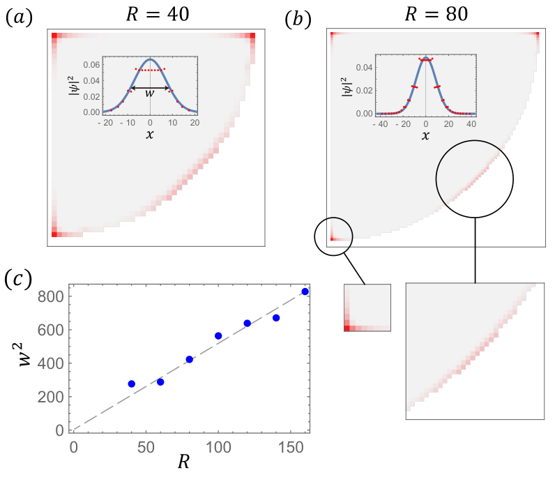
To verify these predictions obtained from the effective surface Hamiltonian, we diagonalize the tight-binding model in Eq.(1) on a finite-size system with the shape of one-quarter cylinder in Fig.7. The direction is taken to be periodic. We find that at , there are four eigenstates with zero energy, with three of them localized at the hinges, and one localized at cylindrical part of the surface. We use Gaussian fit to obtain the width of the state at the cylindrical surface, as shown in the inset of Fig.7. Here is the distance to the center of the zero mode. Define width by the location where the Gaussian curve reduces to half its peak value, then . The fitting shows the wave function profile approaches a Gaussian function when increases, while for small there is deviation from Gaussian due to finite size effect. For and we obtain and respectively. as a function of in various system sizes is shown in Fig.7(c). The linear relation between and indicates and at large system size. Therefore, as the system size increases, the angular width of the state at the cylindrical surface decreases, approaching an effective hinge state. Therefore, the emergence of hinge states as features of higher-order topology does not require the boundaries to preserve the protecting symmetry nor does it require the existence of a physical hinge. Although the computation in Fig.7 is performed for a non-interacting system, the hinge modes are expected to persist under weak interaction due to the presence of a finite surface gap. However, a direct numerical verification of the existence of hinge states in an interacting system with large system size is beyond the scope of this work.
We emphasize that the above conclusions do not imply these hinge states will emerge under arbitrary boundary conditions that break the protecting symmetry. For example, due to the absence of symmetry on the boundary, in principle the hinge states in Fig.1(a) can be removed by superimposing a layer of Chern insulator to the left and right side surfaces respectively. However, this process has to be a large perturbation that closes the surface gap. Our results in Fig.6 and 7 show that if the boundary is obtained by truncating the crystal rather than decorating with another material, then the presence of hinge states is a local property of the boundary, independent of whether the boundary satisfies the global symmetry. In regards of the realization of these hinge states in experiments, this implies the boundary termination of the sample does not need to strictly obey the symmetry and does not require a sharp hinge for these hinge states to be observed.
VII Conclusion
We show that the eigenstates of inverse Green’s function at zero frequency are useful tools in characterizing higher-order topological phases with electronic interaction. In particular, it enables us to compute the topological index of interacting -symmetric second-order topological insulator in a gauge-independent way, and with additional symmetry the topological index the interacting system can be determined by eigenvalues directly, similar to the Fu-Kane formula. This Green’s function-based approach can also be applied to compute the topological index for higher-order topological superconductors. We demonstrate that the hinge states as features of higher-order topology are robust to interaction and deformation of boundaries. If the sample of higher-order topological insulator is sufficiently large and has natural open boundary condition such that its boundaries are obtained by truncating the crystal, the hinge states survive even in the absence of a physical hinge at the boundary. We also propose crystal structures with -preserving magnetic order as possible platforms to realize this higher-order topological phase with electron interactions.
VIII Acknowledgement
This work is supported by the Natural Sciences and Engineering Research Council of Canada (NSERC) and the Center for Quantum Materials at the University of Toronto. H.Y.K acknowledges the support by the Canadian Institute for Advanced Research (CIFAR) and the Canada Research Chairs Program.
Appendix A Details in the derivation of topological indices
A.1 Proof of anti-symmetry
The Pfaffian formula Eq.(8) requires the matrix to be anti-symmetric. We show that is anti-symmetric for every -invariant point such that . Let , we can show that . This is due to , then and . Therefore is an anti-unitary operator similar to the time-reversal operator for spin 1/2 systems which gives rise to Kramers degeneracy. Then for every -invariant momentum we have
| (S1) | |||||
This shows is anti-symmetric, hence its Pfaffian is well-defined.
A.2 Proof of Eq.(12)
We present the derivation that leads to Eq.(12) in the main text. This part follows Ref. Li and Sun 2020b. First we show that the line quantity in Eq.(10) is gauge-invariant, i.e., invariant under gauge transformation where is a unitary matrix and the summation is over the eigenstates of inverse Green’s function with positive eigenvalues. First consider the limit in which and are close to each other. Then . Under the gauge transformation, , . Therefore
This shows that is gauge-invariant when is close to . For a general pair of separated momentum points and , we can divide the path connecting , by small segments . Then . For each small segment is gauge-invariant, therefore is gauge-invariant as well. This gauge-invariance allows us to compute without a smooth gauge.
Next we show that can be related to the topological index . Select a gauge on the straight line such that is smooth and periodic. For each in the region in Fig.1(b), let and then a parallel transport gauge Soluyanov and Vanderbilt 2012 that is smooth in can be defined by
| (S2) |
In this gauge for each , becomes unity, and we get
| (S3) |
Note that if . Therefore, Eq.(12) becomes the winding of the phase of along and , which is equivalent to since contribution along and cancel by periodicity. Therefore, Eq.(12) represents the winding of Pfaffian along , which is equivalent to Eq.(8). This proves Eq.(12) in the parallel transport gauge. Because is gauge-invariant, Eq.(12) should be true in any gauge. This finishes the proof.
References
- Qi and Zhang (2011) Xiao-Liang Qi and Shou-Cheng Zhang, “Topological insulators and superconductors,” Rev. Mod. Phys. 83, 1057–1110 (2011).
- Qi et al. (2008) Xiao-Liang Qi, Taylor L. Hughes, and Shou-Cheng Zhang, “Topological field theory of time-reversal invariant insulators,” Phys. Rev. B 78, 195424 (2008).
- Hasan and Kane (2010) M. Z. Hasan and C. L. Kane, “Colloquium: Topological insulators,” Rev. Mod. Phys. 82, 3045–3067 (2010).
- Fu and Kane (2006) Liang Fu and C. L. Kane, “Time reversal polarization and a adiabatic spin pump,” Phys. Rev. B 74, 195312 (2006).
- Fu et al. (2007) Liang Fu, C. L. Kane, and E. J. Mele, “Topological insulators in three dimensions,” Phys. Rev. Lett. 98, 106803 (2007).
- Fu and Kane (2007) Liang Fu and C. L. Kane, “Topological insulators with inversion symmetry,” Phys. Rev. B 76, 045302 (2007).
- Kane and Mele (2005) C. L. Kane and E. J. Mele, “ topological order and the quantum spin hall effect,” Phys. Rev. Lett. 95, 146802 (2005).
- Benalcazar et al. (2017a) Wladimir A. Benalcazar, B. Andrei Bernevig, and Taylor L. Hughes, “Quantized electric multipole insulators,” Science 357, 61–66 (2017a).
- Benalcazar et al. (2017b) Wladimir A. Benalcazar, B. Andrei Bernevig, and Taylor L. Hughes, “Electric multipole moments, topological multipole moment pumping, and chiral hinge states in crystalline insulators,” Phys. Rev. B 96, 245115 (2017b).
- Schindler et al. (2018a) Frank Schindler, Ashley M. Cook, Maia G. Vergniory, Zhijun Wang, Stuart S. P. Parkin, B. Andrei Bernevig, and Titus Neupert, “Higher-order topological insulators,” Sci. Adv 4 (2018a), 10.1126/sciadv.aat0346.
- Ahn and Yang (2019) Junyeong Ahn and Bohm-Jung Yang, “Symmetry representation approach to topological invariants in -symmetric systems,” Phys. Rev. B 99, 235125 (2019).
- (12) Benjamin J. Wieder and B. Andrei Bernevig, “The Axion Insulator as a Pump of Fragile Topology,” arXiv:1810.02373 .
- Ezawa (2018a) Motohiko Ezawa, “Strong and weak second-order topological insulators with hexagonal symmetry and 3 index,” Phys. Rev. B 97, 241402 (2018a).
- Ezawa (2018b) Motohiko Ezawa, “Magnetic second-order topological insulators and semimetals,” Phys. Rev. B 97, 155305 (2018b).
- Fang and Fu (2015) Chen Fang and Liang Fu, “New classes of three-dimensional topological crystalline insulators: Nonsymmorphic and magnetic,” Phys. Rev. B 91, 161105 (2015).
- van Miert and Ortix (2018) Guido van Miert and Carmine Ortix, “Higher-order topological insulators protected by inversion and rotoinversion symmetries,” Phys. Rev. B 98, 081110 (2018).
- Khalaf (2018) Eslam Khalaf, “Higher-order topological insulators and superconductors protected by inversion symmetry,” Phys. Rev. B 97, 205136 (2018).
- Kooi et al. (2018) Sander H. Kooi, Guido van Miert, and Carmine Ortix, “Inversion-symmetry protected chiral hinge states in stacks of doped quantum hall layers,” Phys. Rev. B 98, 245102 (2018).
- Călugăru et al. (2019) Dumitru Călugăru, Vladimir Juričić, and Bitan Roy, “Higher-order topological phases: A general principle of construction,” Phys. Rev. B 99, 041301 (2019).
- Varjas et al. (2015) Dániel Varjas, Fernando de Juan, and Yuan-Ming Lu, “Bulk invariants and topological response in insulators and superconductors with nonsymmorphic symmetries,” Phys. Rev. B 92, 195116 (2015).
- Ezawa (2019) Motohiko Ezawa, “Second-order topological insulators and loop-nodal semimetals in transition metal dichalcogenides xte2 (x = mo, w),” Sci. Rep 9, 5286 (2019).
- Wang et al. (2019) Zhijun Wang, Benjamin J. Wieder, Jian Li, Binghai Yan, and B. Andrei Bernevig, “Higher-order topology, monopole nodal lines, and the origin of large fermi arcs in transition metal dichalcogenides (),” Phys. Rev. Lett. 123, 186401 (2019).
- Song et al. (2017) Zhida Song, Zhong Fang, and Chen Fang, “-dimensional edge states of rotation symmetry protected topological states,” Phys. Rev. Lett. 119, 246402 (2017).
- Matsugatani and Watanabe (2018) Akishi Matsugatani and Haruki Watanabe, “Connecting higher-order topological insulators to lower-dimensional topological insulators,” Phys. Rev. B 98, 205129 (2018).
- Langbehn et al. (2017) Josias Langbehn, Yang Peng, Luka Trifunovic, Felix von Oppen, and Piet W. Brouwer, “Reflection-symmetric second-order topological insulators and superconductors,” Phys. Rev. Lett. 119, 246401 (2017).
- Yue et al. (2019) Changming Yue, Yuanfeng Xu, Zhida Song, Hongming Weng, Yuan-Ming Lu, Chen Fang, and Xi Dai, “Symmetry-enforced chiral hinge states and surface quantum anomalous hall effect in the magnetic axion insulator bi2-xsmxse3,” Nat. Phys 15, 577–581 (2019).
- Hsu et al. (2018) Chen-Hsuan Hsu, Peter Stano, Jelena Klinovaja, and Daniel Loss, “Majorana kramers pairs in higher-order topological insulators,” Phys. Rev. Lett. 121, 196801 (2018).
- Queiroz and Stern (2019) Raquel Queiroz and Ady Stern, “Splitting the hinge mode of higher-order topological insulators,” Phys. Rev. Lett. 123, 036802 (2019).
- Xue et al. (2019) Haoran Xue, Yahui Yang, Fei Gao, Yidong Chong, and Baile Zhang, “Acoustic higher-order topological insulator on a kagome lattice,” Nat. Mater 18, 108–112 (2019).
- Geier et al. (2018) Max Geier, Luka Trifunovic, Max Hoskam, and Piet W. Brouwer, “Second-order topological insulators and superconductors with an order-two crystalline symmetry,” Phys. Rev. B 97, 205135 (2018).
- Schindler et al. (2018b) Frank Schindler, Zhijun Wang, Maia G. Vergniory, Ashley M. Cook, Anil Murani, Shamashis Sengupta, Alik Yu Kasumov, Richard Deblock, Sangjun Jeon, Ilya Drozdov, Hélène Bouchiat, Sophie Guéron, Ali Yazdani, B. Andrei Bernevig, and Titus Neupert, “Higher-order topology in bismuth,” Nat. Phys 14, 918–924 (2018b).
- Trifunovic and Brouwer (2019) Luka Trifunovic and Piet W. Brouwer, “Higher-order bulk-boundary correspondence for topological crystalline phases,” Phys. Rev. X 9, 011012 (2019).
- Ghorashi et al. (2019) Sayed Ali Akbar Ghorashi, Xiang Hu, Taylor L. Hughes, and Enrico Rossi, “Second-order dirac superconductors and magnetic field induced majorana hinge modes,” Phys. Rev. B 100, 020509 (2019).
- Nag et al. (2021) Tanay Nag, Vladimir Juričić, and Bitan Roy, “Hierarchy of higher-order floquet topological phases in three dimensions,” Phys. Rev. B 103, 115308 (2021).
- Ghosh et al. (2021) Arnob Kumar Ghosh, Tanay Nag, and Arijit Saha, “Hierarchy of higher-order topological superconductors in three dimensions,” Phys. Rev. B 104, 134508 (2021).
- Trifunovic and Brouwer (2021) Luka Trifunovic and Piet W. Brouwer, “Higher-order topological band structures,” physica status solidi (b) 258, 2000090 (2021).
- Benalcazar et al. (2019) Wladimir A. Benalcazar, Tianhe Li, and Taylor L. Hughes, “Quantization of fractional corner charge in -symmetric higher-order topological crystalline insulators,” Phys. Rev. B 99, 245151 (2019).
- Fang and Cano (2021) Yuan Fang and Jennifer Cano, “Filling anomaly for general two- and three-dimensional symmetric lattices,” Phys. Rev. B 103, 165109 (2021).
- Lee et al. (2022) Wonjun Lee, Gil Young Cho, and Byungmin Kang, “Many-body quadrupolar sum rule for higher-order topological insulators,” Phys. Rev. B 105, 155143 (2022).
- Yu et al. (2011) Rui Yu, Xiao Liang Qi, Andrei Bernevig, Zhong Fang, and Xi Dai, “Equivalent expression of topological invariant for band insulators using the non-abelian berry connection,” Phys. Rev. B 84, 075119 (2011).
- Franca et al. (2018) S. Franca, J. van den Brink, and I. C. Fulga, “An anomalous higher-order topological insulator,” Phys. Rev. B 98, 201114 (2018).
- Bouhon et al. (2019) Adrien Bouhon, Annica M. Black-Schaffer, and Robert-Jan Slager, “Wilson loop approach to fragile topology of split elementary band representations and topological crystalline insulators with time-reversal symmetry,” Phys. Rev. B 100, 195135 (2019).
- Fang et al. (2012) Chen Fang, Matthew J. Gilbert, and B. Andrei Bernevig, “Bulk topological invariants in noninteracting point group symmetric insulators,” Phys. Rev. B 86, 115112 (2012).
- Bradlyn et al. (2017) Barry Bradlyn, L. Elcoro, Jennifer Cano, M. G. Vergniory, Zhijun Wang, C. Felser, M. I. Aroyo, and B. Andrei Bernevig, “Topological quantum chemistry,” Nature 547, 298 EP – (2017).
- Po et al. (2017) Hoi Chun Po, Ashvin Vishwanath, and Haruki Watanabe, “Symmetry-based indicators of band topology in the 230 space groups,” Nat. Commun 8, 50 (2017).
- Kruthoff et al. (2017) Jorrit Kruthoff, Jan de Boer, Jasper van Wezel, Charles L. Kane, and Robert-Jan Slager, “Topological classification of crystalline insulators through band structure combinatorics,” Phys. Rev. X 7, 041069 (2017).
- Khalaf et al. (2018) Eslam Khalaf, Hoi Chun Po, Ashvin Vishwanath, and Haruki Watanabe, “Symmetry indicators and anomalous surface states of topological crystalline insulators,” Phys. Rev. X 8, 031070 (2018).
- Ono and Watanabe (2018) Seishiro Ono and Haruki Watanabe, “Unified understanding of symmetry indicators for all internal symmetry classes,” Phys. Rev. B 98, 115150 (2018).
- Song et al. (2018) Zhida Song, Tiantian Zhang, Zhong Fang, and Chen Fang, “Quantitative mappings between symmetry and topology in solids,” Nature Communications 9, 3530 (2018).
- Zhang et al. (2019) Tiantian Zhang, Yi Jiang, Zhida Song, He Huang, Yuqing He, Zhong Fang, Hongming Weng, and Chen Fang, “Catalogue of topological electronic materials,” Nature 566, 475–479 (2019).
- Tang et al. (2019) Feng Tang, Hoi Chun Po, Ashvin Vishwanath, and Xiangang Wan, “Comprehensive search for topological materials using symmetry indicators,” Nature 566, 486–489 (2019).
- Vergniory et al. (2019) M. G. Vergniory, L. Elcoro, Claudia Felser, Nicolas Regnault, B. Andrei Bernevig, and Zhijun Wang, “A complete catalogue of high-quality topological materials,” Nature 566, 480–485 (2019).
- Fidkowski and Kitaev (2010) Lukasz Fidkowski and Alexei Kitaev, “Effects of interactions on the topological classification of free fermion systems,” Phys. Rev. B 81, 134509 (2010).
- Resta (1998) Raffaele Resta, “Quantum-mechanical position operator in extended systems,” Phys. Rev. Lett. 80, 1800–1803 (1998).
- Slager et al. (2015) Robert-Jan Slager, Louk Rademaker, Jan Zaanen, and Leon Balents, “Impurity-bound states and green’s function zeros as local signatures of topology,” Phys. Rev. B 92, 085126 (2015).
- Shiozaki et al. (2018) Ken Shiozaki, Hassan Shapourian, Kiyonori Gomi, and Shinsei Ryu, “Many-body topological invariants for fermionic short-range entangled topological phases protected by antiunitary symmetries,” Phys. Rev. B 98, 035151 (2018).
- Kang et al. (2019) Byungmin Kang, Ken Shiozaki, and Gil Young Cho, “Many-body order parameters for multipoles in solids,” Phys. Rev. B 100, 245134 (2019).
- Wheeler et al. (2019) William A. Wheeler, Lucas K. Wagner, and Taylor L. Hughes, “Many-body electric multipole operators in extended systems,” Phys. Rev. B 100, 245135 (2019).
- Kudo et al. (2019) Koji Kudo, Haruki Watanabe, Toshikaze Kariyado, and Yasuhiro Hatsugai, “Many-body chern number without integration,” Phys. Rev. Lett. 122, 146601 (2019).
- Kang et al. (2021) Byungmin Kang, Wonjun Lee, and Gil Young Cho, “Many-body invariants for chern and chiral hinge insulators,” Phys. Rev. Lett. 126, 016402 (2021).
- Wang et al. (2012) Zhong Wang, Xiao-Liang Qi, and Shou-Cheng Zhang, “Topological invariants for interacting topological insulators with inversion symmetry,” Phys. Rev. B 85, 165126 (2012).
- Wang and Zhang (2012a) Zhong Wang and Shou-Cheng Zhang, “Simplified topological invariants for interacting insulators,” Phys. Rev. X 2, 031008 (2012a).
- Wang and Zhang (2012b) Zhong Wang and Shou-Cheng Zhang, “Strongly correlated topological superconductors and topological phase transitions via green’s function,” Phys. Rev. B 86, 165116 (2012b).
- Zhao et al. (2021) Peng-Lu Zhao, Xiao-Bin Qiang, Hai-Zhou Lu, and X. C. Xie, “Coulomb instabilities of a three-dimensional higher-order topological insulator,” Phys. Rev. Lett. 127, 176601 (2021).
- (65) Yu-Wen Lee and Min-Fong Yang, “Comment on "coulomb instabilities of a three-dimensional higher-order topological insulator",” arXiv:2202.01642 .
- (66) Jing-Rong Wang and Chang-Jin Zhang, “Fate of higher-order topological insulator under coulomb interaction,” arXiv:2202.03417 .
- Li and Sun (2020a) Heqiu Li and Kai Sun, “Pfaffian formalism for higher-order topological insulators,” Phys. Rev. Lett. 124, 036401 (2020a).
- Li and Sun (2020b) Heqiu Li and Kai Sun, “Topological insulators and higher-order topological insulators from gauge-invariant one-dimensional lines,” Phys. Rev. B 102, 085108 (2020b).
- Wang et al. (2018) Yuxuan Wang, Mao Lin, and Taylor L. Hughes, “Weak-pairing higher order topological superconductors,” Phys. Rev. B 98, 165144 (2018).
- Soluyanov and Vanderbilt (2012) Alexey A. Soluyanov and David Vanderbilt, “Smooth gauge for topological insulators,” Phys. Rev. B 85, 115415 (2012).