The Subtype-Free Average Causal Effect for Heterogeneous Disease Etiology
Abstract
Studies have shown that the effect an exposure may have on a disease can vary for different subtypes of the same disease. However, existing approaches to estimate and compare these effects largely overlook causality. In this paper, we study the effect smoking may have on having colorectal cancer subtypes defined by a trait known as microsatellite instability (MSI). We use principal stratification to propose an alternative causal estimand, the Subtype-Free Average Causal Effect (SF-ACE). The SF-ACE is the causal effect of the exposure among those who would be free from other disease subtypes under any exposure level. We study non-parametric identification of the SF-ACE, and discuss different monotonicity assumptions, which are more nuanced than in the standard setting. As is often the case with principal stratum effects, the assumptions underlying the identification of the SF-ACE from the data are untestable and can be too strong. Therefore, we also develop sensitivity analysis methods that relax these assumptions. We present three different estimators, including a doubly-robust estimator, for the SF-ACE. We implement our methodology for data from two large cohorts to study the heterogeneity in the causal effect of smoking on colorectal cancer with respect to MSI subtypes.
Keywords: principal stratification, survivor average causal effect, competing risks, molecular pathological epidemiology
1 Introduction
In recent decades, it has become clear that many diseases that share general clinical characteristics evolve through a range of heterogeneous molecular pathologic processes, which may be affected differently by the same exposure. For this reason, classifying a disease into subtypes according to criteria based on molecular characteristics can improve our etiologic understanding of the disease (Ogino et al. 2016).
In this paper, we consider the causal effect smoking may have on having colorectal cancer (CRC). One well-established CRC subtype classification is based on microsatellite instability (MSI). The two mutually-exclusive subtypes are MSI-high (approximately 15% of the cases) and non-MSI-high (approximately 85%). Smoking has been found to be a strong risk factor for the MSI-high subtype, while weaker evidence was found that smoking is a risk factor for the non-MSI-high subtype (Carr et al. 2018; Amitay et al. 2020).
To study etiologic heterogeneity, researchers often use a multinomial regression model in which being healthy or having each of the disease subtypes form the possible values of the outcome. However, the multinomial regression parameters do not correspond to well-defined causal effects, because the multinomial regression parameters are equivalent to the parameters obtained from a series of logistics regressions, each comparing one disease subtype to the healthy controls, resulting in selection bias (Nevo et al. 2021).
This form of bias is not limited to subtype comparisons and is not unique to multinomial regression. More generally, competing events create a challenge in making causal statements. Section 4.2 reviews related approaches and considers their applicability in our setup (Young et al. 2020; Stensrud et al. 2020; Nevo et al. 2021).
In this paper, we use data from two large cohorts to study well-defined and relevant estimands representing the effect of smoking on the two CRC subtypes. We propose an alternative estimand, inspired by the Survivor Average Causal Effect () (Zhang and Rubin 2003; Rubin 2006; Zehavi and Nevo 2021). The is a causal effect typically-used to overcome the problem of truncation by death, which occurs when an outcome of interest is undefined for individuals who died before their outcome could be measured. The is defined using principal stratification (Robins 1986; Frangakis and Rubin 2002) as the average causal effect of a treatment among individuals that would have survived under both treatment/exposure values. The is not identifiable from the data under standard assumptions. Approaches to identify and estimate include relying on additional strong assumptions, performing sensitivity analyses, and obtaining bounds.
Our proposed approach is based on the same idea as the . First, we define principal strata with respect to the potential outcomes of other disease subtypes. Then, we define the Subtype-Free Average Causal Effect () to be the average causal effect of the exposure on one disease subtype among the individuals who would have been free of the other MSI disease subtype under either exposure level (smoking status).
One commonly-made assumption in truncation-by-death problems is Monotonicity, namely that treatment/exposure cannot hurt survival (Zhang and Rubin 2003). In the setting of disease heterogeneity with two subtypes, the definition of Monotonicity is more nuanced for two reasons. First, the assumption needs to be made (or not) for each subtype separately. Second, the disease could occur under both exposure statuses, but the subtype may differ. We term this phenomenon exposure-induced subtype switching and show it plays a key role in the (lack of) identification of the . We further show that unlike the setting, the is non-parametrically identifiable under certain Monotonicity assumptions. Under weaker Monotonicity assumptions, the is no longer identifiable. For this scenario, we develop a sensitivity analysis approach as a function of the unidentifiable exposure-induced subtype switching probabilities.
We consider three estimators. The first two, standardization-based estimator and an inverse probability of treatment weighting (IPTW) estimator, may rely on parametric modeling assumptions. We therefore present a doubly-robust (DR) estimator that will be consistent if at least one of two models, but not necessarily both, is correctly specified.
The rest of the paper is organized as follows. Section 2 describes the epidemiologic problem and the available data. Section 3 presents the notations and the causal framework. Section 4 reviews existing approaches for etiologic disease heterogeneity and discuss available causal estimands. Section 5 presents a detailed study of the proposed causal estimand, the , including its interpretation, assumptions needed for its identification, sensitivity analyses and estimation. Section 6 summarizes the results of our simulation studies. Section 7 presents various analyses of the data to study the causal effect of smoking on the two CRC subtypes. Final conclusions are given in Section 8. The R package TheSFACE is available from CRAN implements our methodology. Reproducibility materials are available from https://github.com/amitSasson/SFACE_Reproduce.
2 Data and problem description
We use data from two large US cohorts. The Nurses Health Study (NHS) was established in 1976 and consists of female nurses aged 30–55 at the beginning of follow-up. The Health Professionals Follow-up Study (HPFS) was established in 1986 and consists of male health professionals aged 40–75 at the beginning of follow-up. Participants answered biennial questionnaires about lifestyle, medical and other health-related information every two years. CRC diagnoses were reported by study participants. Formalin-fixed paraffin-embedded tumor tissue specimens were retrieved from hospitals across the US, and a CRC diagnosis was confirmed by the study pathologist (S.O.), who also conducted analyses to determine the MSI status. Further details can be found in Ugai et al. 2022 and references therein.
We set the baseline to be age 60, and define the exposure to be ever versus never smoking by age 60. Such binary exposure definitions are often used to minimize recall bias and measurement error. The outcome was CRC by age 70, subtyped by MSI status. Age 70 was chosen to minimize the impact of death as a competing event.
We removed from the data people who were older than 60 when enrolled in the study, or people who died, had CRC, or were lost to follow up before age 60. As in Ugai et al. 2022, we also removed people with missing baseline smoking data. In total, we were left with 114,947 people at baseline. Then, we removed 5,132 people (4.4%) who have died, without being diagnosed, prior to age 70. We were left with a final sample of 109,815. In this sample, 17,854 people were CRC-free and younger than 70 when the last questionnaire was collected (out of which 94.8% were older than 65). We treated them as CRC-free at age 70, and examined how it may affected our results by considering alternative analyses.
In our sample, the number of exposed (ever smoking) was 58,432 (53.3%) and the number of CRC cases by age 70 was 961 (0.9%). Out of them, 358 were diagnosed with non-MSI-high CRC (37.3%) and 61 were diagnosed with MSI-high CRC (6.3%). The subtype was missing for the remaining 542 (56.4%) diagnosed participants, as is often the case in such studies (Nevo et al. 2018; Liu et al. 2018). To have a clear presentation of the issues at end, we develop our theory and methodology under the assumption that subtypes are known for all disease cases. We address the issue of missing subtypes in our analysis in Section 7 using inverse probability weighting (Liu et al. 2018).
The NHS and HPFS cohorts include a vast number of covariates collected through biennial questionnaires. Table C.7 in the Appendix provides information on key baseline confounders we adjusted for in our analyses: gender (male/female), regular aspirin use (yes/no), first-degree family history of CRC (yes/no), history of lower endoscopy (yes/no), physical activity level (mean metabolic equivalent task score hours per week), body mass index (categorical), alcohol intake (g/day) and total calorie intake (kcal/day).
3 Preliminaries
Using the potential outcomes framework, let denote the potential disease status had the exposure of individual been set to for . In our study, indicates no smoking by age 60 (as captured by the cohort data), while indicates ever smoking by age 60. If individual would have been diagnosed with disease subtype under exposure value , then , and if they would be disease-free under , then . Let also indicate whether individual is diagnosed with disease type under . Note that because the subtypes are mutually exclusive, . In our study, , subtype 1 is non-MSI-high CRC, and subtype 2 is MSI-high CRC. So, for example, if person would have been diagnosed with non-MSI-high CRC by age 70 had they not been smoking by age 60.
Throughout the paper, we assume there is no interference between individuals and that there are no multiple versions of the exposure leading to different potential outcomes. Under these assumptions, known collectively as the stable unit treatment value assumption (SUTVA), the observed disease status for person , hereafter denoted by , with observed exposure value , equals to the appropriate potential outcome for that person. That is, (and ). The latter is also known as the consistency assumption.
As in many observational studies, we also assume weak ignorability, namely that rich enough data were collected as part of the NHS and HPFS cohorts such that for a vector of measured covariates , we have for . Another typically needed assumption for identification of causal effects is positivity, meaning that the exposure assignment probability is positive for and for all .
In summary, the observed data consists of i.i.d copies sampled from the distribution of , that can be equivalently represented as .
4 Review of existing approaches
A principled approach to causal inference typically starts with a definition of causal effects of interest, followed by the assumptions needed for their identification from observed data, and only then statistical models are discussed. However, as the existing approaches employed in practice for studying etiologic heterogeneity are model-based and are not grounded in the causal inference paradigm, we start with reviewing these models (Section 4.1). Then, we discuss relevant causal effects arising in the presence of competing events (Section 4.2).
4.1 Statistical models for disease heterogeneity
Let , , be the probability of subtype disease (or being subtype-free for ) among those with exposure and confounders . Let also . A commonly-used approach for studying etiologic heterogeneity is built upon the multinomial regression model
| (1) |
for and . Under this model, is the odds ratio (OR) between the exposure and the observed subtype-specific outcome compared with not having the disease, that is, The parameter also approximates the risk ratio (RR) when the disease is rare, as in our study. Model (1) was also extended for studies within which subtypes were not a-priori known and may be defined using multiple, possibly mis-meausred, biomarkers (Chatterjee 2004; Wang et al. 2015; Nevo et al. 2016). See also Wang et al. 2016; Zabor and Begg 2017 for a survey of and comparison between methods based on this and similar models.
Estimation of Model (1) parameters is typically carried out by standard maximum likelihood approach, with some exceptions when further complications arise (Chatterjee 2004; Nevo et al. 2016, e.g.,). In practice, researchers are often interested in whether there is heterogeneity in the effects of across disease subtypes. When the null hypothesis is rejected, researchers conclude that the exposure contributes to the risk of at least one subtype differently from its contribution to the risk of other subtypes.
A recently-proposed alternative approach postulates logistic regressions, each comparing a subtype disease to the alternative of being free of that subtype, that is, being either disease-free or diagnosed with the disease, but of a different subtype (Sun et al. 2017). Formally, these models can be expressed by
| (2) |
for . Under this model, is the OR between the exposure and the observed indicator of subtype-specific outcome ; that is, Because fitting these models separately may result in , estimation of the parameters in (2) calls for constrained maximization of the models’ likelihood. A more computationally attractive approach, developed by Sun et al. 2017, uses constrained Bayesian estimation, and limits the posterior distribution of the parameter vector to have positive mass only for parameter values such that .
Comparing models (1) and (2), it has been recently argued (Sun et al. 2017) that variation in across the subtypes (across ) is not a satisfactory measure of etiologic heterogeneity, because the parameter space of a multinomial regression model requires a risk factor for one subtype to be a risk factor for the other subtypes, and that may be preferred, although this issue was also debated (Begg et al. 2018; Sun et al. 2018).
4.2 Causal effects for competing risks
To fix ideas, we focus on the effect of on , the first subtype, and start with a naïve approach that does not correspond to a causal effect. Researchers may opt for a comparison of the subtype 1 proportion of cases at each exposure level only among individuals who are free of other disease subtypes. When researchers also adjust for the confounders , their statistical estimand on the difference scale is
| (3) |
and can be analogously defined on the RR or OR scales. Because model (1) is equivalent to separate logistic regression models, each comparing one disease subtype to the disease-free individuals (Wang et al. 2016), then is the OR analogue of (3), and approximates the RR as CRC is a rare disease. However, (3) does not correspond to a causal effect, because of selection bias due to common causes of the different subtypes (Nevo et al. 2021). These common causes cannot be classified as classical confounders, as they can be independent of the exposure. If these common causes are also mediators of an exposure-subtype mechanisms that are shared between more than one subtype, even had they been observed, adjusting for them would have eliminated part of the causal effect of the exposure on the subtype (Nevo et al. 2021). Importantly, because MSI-high and non-MSI-high are subtypes of the same disease, CRC, they are likely to have unknown and/or unmeasured common causes.
Young et al. 2020 considered possible causal estimands in the presence of competing events. The total effect, contrasts the population-level subtype risk had the entire population been exposed, with the population-level subtype risk had the entire population were unexposed. In the presence of measured confounders, this effect is identified from the observed data under SUTVA, weak ignorability and positivity by
| (4) |
Unlike (3), the definition of does not involve conditioning on the post-exposure variable of not having the other subtypes. Note also that if model (2) is correctly specified, is the total effect for subtype on the OR/RR scales.
However, despite being a valid causal effect, it does not suffice to describe exposure effects in the presence of etiologic disease heterogeneity. The total effect of on , for example, includes the effect caused by changes in , , or, in other words, is sensitive to the phenomenon of exposure-induced subtype switching. For example, assume some individuals would have been diagnosed with subtype 1 under and would have been diagnosed with subtype 2 under , while the rest of the population will be free of subtype 1 for all values. Then, the total effect on subtype 1 will be negative, , and it would appear as if the exposure protects from subtype 1, even though the individuals “protected” by would still have the disease, just of another subtype.
The direct effect (Young et al. 2020) is the causal effect comparing subtype 1 rates under two hypothetical joint interventions. The first sets the exposure to and eliminates the possibility of disease subtypes other than subtype 1 disease, and the second sets the exposure to and also eliminates risks of other disease subtypes. This approach is, however, irrelevant for our study, because an intervention eliminating the risk of a particular CRC subtype is not currently available and is not expected to be in the near future.
Another alternative considers the separable effects (Stensrud et al. 2020), which rely on a conceptual separation of the exposure into the components affecting each disease subtype. Such separation requires profound understanding of the mechanisms leading to each CRC subtype. Furthermore, the conditions needed for identifiability of these effects are violated if there are unobserved common causes of both disease subtypes (Stensrud et al. 2020). Such common causes are expected to exist in our study and in many disease subtype studies (Nevo et al. 2021).
5 The Subtype-Free Average Causal Effect
Our focus in this paper is on the common scenario of two disease subtypes (), as in our study. We propose a new estimand, inspired by the (Rubin 2006). We define the on the difference scale by
| (5) |
and analogously define
to be the on the RR scale. The is the average causal effect among the individuals that would have been free of disease subtype 2 under either exposure level (i.e., regardless of smoking status). Similarly to , let
be the average causal effect on the difference scale of on among the individuals that would have been free of disease subtype 1 under either exposure level. Let also be the analogous causal effect on the RR scale. Disease heterogeneity studies often focus on whether the exposure has the same effect on both disease subtypes. For investigating the heterogeneity of the causal effects, one can use and test the null hypothesis of versus the alternative of .
5.1 Interpretation of the
As explained in Section 4.2, competing events present a challenge in defining causal estimands that shed light on the scientific question of interest. The presents another source of information. A positive value means that in the sub-population who would have been free of MSI-high CRC regardless of their smoking status, we will expect more non-MSI-high CRC cases had the entire sub-population smoked compared to the scenario the entire sub-population did not smoke before age 60.
Therefore, the offers a way to circumvent non-zero causal effects due to exposure-induced subtype switching. Nevertheless, the above appealing advantage does not come without a price. One disadvantage is that the is defined in a latent subset of the population. This is a general problem with principal stratification approaches. A second, related, issue is that when contrasting and , we contrast effects defined in two overlapping, but not identical, sub-populations. The is defined within the sub-population , and the is defined within the sub-population .
Thus, a non-zero captures changes that might be due to the different population, and as a result, the exact source of heterogeneity in the causal effect is not revealed. Instead, a non-zero presents evidence of heterogeneity and calls for further investigation. Lastly but importantly, in rare disease scenarios, such as CRC, this problem is less concerning because the two sub-populations and have almost perfect overlap, as those who would not have CRC of any subtype under any exposure value belong to both groups and comprise the vast majority of the population.
5.2 Identifiability
Similar to the in truncation-by-death scenarios, the is not identifiable from the data under the standard assumptions of SUTVA, weak ignorability and positivity. One commonly-made assumption when targeting the SACE is Monotonicity (Zhang and Rubin 2003), stating that treatment cannot hurt survival. In our study, the definition and plausibility of Monotonicity-like assumptions are more nuanced, and, as it turns out, resulting in new insights regarding principal causal effects and their identification in a competing risks setup. We start with the definition of Subtype Monotonicity (S-Monotonicity).
Assumption 1
Subtype Monotonicity (S-Monotonicity): .
S-Monotonicity states that an individual that would have been diagnosed with disease subtype under no exposure (never smoking), would have also been diagnosed with disease subtype under exposure (ever smoking). Therefore, an individual who would have been free of disease subtype under exposure, would have also been free of disease subtype under no exposure. In other words, S-Monotonicity asserts that the exposure cannot prevent the subtype -specific disease. S-Monotonicity trivially holds if the exposure does not affect the outcome at all, and can be easily modified to address scenarios in which the exposure is suspected to have a protective effect.
Importantly, S-Monotonicity is a subtype-specific assumption. It can hold for both subtypes, for one subtype, or for none of them. Interestingly, we show in Section A of the Appendix that under S-Monotonicity for both subtypes, the equals to the total effect . When the effects are defined on the difference scale, this equality does not hold.
It is clear from the above that the is identifiable from the data under SUTVA, weak ignorability, positivity, and S-Monotonicity for both subtypes. The following proposition establishes identification of , and presents identification formulas under either standardization or IPTW (Hernán and Robins 2020).
Proposition 1
Under SUTVA, weak ignorability, positivity, and S-Monotonicity for subtypes , the is identifiable from the observed data by
| (6) | ||||
| using standardization, or via IPTW by | ||||
| (7) |
The proofs and analogous expressions for , , and for causal contrasts on the RR scale are all given in Section A of the Appendix. Estimation based on these identification formulas is discussed in Section 5.5.
5.3 Relaxing S-Monotonicity
Assuming S-Monotonicity for both subtypes might be too restrictive, even if we believe the exposure cannot protect from the outcome, as S-Monotonicity disallows subtype switching for any individual in the population. For example, consider the scenario the exposure is believed to increase non-MSI-high CRC risk but not MSI-high CRC risk. If individual would have been diagnosed with MSI-high CRC when unexposed, then under S-Monotonicity for MSI-high CRC, it will be impossible for individual to be diagnosed with non-MSI-high CRC when exposed. This is even though the exposure is a risk factor only for non-MSI-high CRC.
Therefore, we consider a weaker assumption, termed Disease Monotonicity (D-Monotonicity), that states that an individual who would have been diagnosed with disease subtype under no exposure, would have also been diagnosed with the disease under exposure, but not necessarily with the same subtype.
Assumption 2
Disease Monotonicity (D-Monotonicity): .
D-Monotonicity keeps the premise that the exposure cannot protect from the disease while being less restrictive than S-Monotonicity. As with S-Monotonicity, D-Monotonicity can be modified for scenarios where the exposure is suspected to have a protective effect.
For each disease subtype, we may assume S-Monotonicity, D-Monotonicity, or neither. With two disease subtypes, we have eight different combinations of possible assumptions. Under each combination, certain potential outcome profiles of are assumed to be absent from the population. For example, under S-Monotonicity for subtype 1, there is no one in the population with . Note also that because the subtypes are mutually exclusive, it is impossible to have regardless of the taken monotonicity assumptions.
Table 1 presents the nine possible potential outcome profiles, and specifies whether each profile exists under four different combinations of assumptions. This table demonstrates that the exact implications of the different monotonicity assumptions on the potential outcomes in the population are quite explicit. The observed data, however, does not hold all the information required for classifying each individual into their potential outcome profile. Table A.1 in Section A of the Appendix specifies the possible profiles for each participant according to their observed under each of the four combinations of assumptions.
| Potential outcomes profiles | Monotonicity assumptions | ||||
| Profile | S-Mono S-Mono | D-Mono D-Mono | S-Mono D-Mono | D-Mono S-Mono | |
|---|---|---|---|---|---|
| 0 | ✓ | ✓ | ✓ | ✓ | |
| 1 | ✓ | ✓ | ✓ | ✓ | |
| 2 | ✗ | ✗ | ✗ | ✗ | |
| 3 | ✓ | ✓ | ✓ | ✓ | |
| 4 | ✗ | ✗ | ✗ | ✗ | |
| 5 | ✓ | ✓ | ✓ | ✓ | |
| 6 | ✓ | ✓ | ✓ | ✓ | |
| 7 | ✗ | ✓ | ✗ | ✓ | |
| 8 | ✗ | ✓ | ✓ | ✗ | |
5.4 A sensitivity analysis approach
By Proposition 1, under S-Monotonicity for both disease subtypes, the , and are identifiable from the observed data distribution. If we replace S-Monotonicity with D-Monotonicity or with no monotonicity assumption for at least one subtype, then the causal effects are no longer identifiable, and does not equal to the .
Therefore, we take a sensitivity analysis approach, as is common when studying causal effects under untestable assumptions. Let be the proportion of individuals who would have been diagnosed with disease subtype 2 when exposed, out of the individuals who would have been diagnosed with disease subtype 1 when unexposed. That is, is the probability of exposure-induced subtype switching from subtype 1 to subtype 2. Note that under S-Monotonicity for subtype 1 and under D-Monotonicity for subtype 1. Let also be the subtype-switching probability from subtype 2 to subtype 1. While and are not identifiable from the observed data, they can be bounded. Specifically, because , a data-driven upper bound for is . Similarly, .
The following two propositions demonstrate that the subtype-switching probabilities play a key role in the identification of the whenever the S-Monotonicity assumptions are not met. Proposition 2 shows that (a) under D-Monotonicity for subtype 1 and S-Monotonicity for subtype 2, both the and are identifiable as functions of , (b) under D-Monotonicity for subtype 2 and S-Monotonicity for subtype 1, the and are identifiable as functions of , and (c) under D-Monotonicity for both subtypes, the s are identifiable as functions of and .
Proposition 2
Under SUTVA, weak ignorability, positivity and D-Monotonicity for both subtypes, the is identifiable from the data by
| (8) | ||||
| using standardization, or via IPTW by | ||||
| (9) |
The identification of is analogous.
The proof is given in Section A of the Appendix. Of note is that if one further assumes S-Monotonicity for one of the subtypes (say subtype 2), then an identification formula of is obtained by setting the appropriate (say ) to zero in (8) and (9). A second remark is that, technically, results (8) and (9) require D-Monotonicity for subtype 2 only, and similarly, the identification for subtype 2 requires D-Monotonicity for subtype 1 only. In Section A of the Appendix, we present further identification results for under D-Monotonicity for one subtype only or without any monotonicity assumptions, and show that in these cases and do not suffice for identification of .
Turning to the RR scale, Proposition 3 asserts that is identifiable as a function of and and the observed data without imposing any monotonicity assumptions.
Proposition 3
Under SUTVA, weak ignorability and positivity, the is identifiable via standardization by
or using IPTW,
The identification of is analogous.
The proof is given in Section A of the Appendix.
Propositions 2 and 3 serve as basis for our proposed sensitivity analyses. Researchers first decide what is the effect scale of interest, and then for which if any of the two subtypes the S-Monotonicity or D-Monotonicity assumptions are plausible. Then, depending on the taken assumptions, they may set or to zero, and estimate the and as a function of and/or . Such an analysis can reveal how sensitive the results are to different levels of exposure-induced subtype switching. We implement these analyses in our study of smoking effect on CRC MSI subtypes in Section 7.
5.5 Estimation
Recall that for each individual , the observed data are () or equivalently (). Estimation of and from the data alongside the sensitivity analyses for the S-Monotonicity assumptions require estimation of , for the standardization-based formulas, or for the IPTW-based identification formulas. Expectations over or are estimated by taking the sample analogues.
Non-parametric estimation of or when the vector of measured confounders is of high dimension or includes many continuous variables could be a difficult task, that will yield an estimator with a too large variance to be able to derive conclusions from the data. Therefore, parametric estimation might be a better option, and also aligns with the models used in practice and that were presented in Section 4.1. We first discuss parametric estimation, before implementing a DR estimator that will be consistent even if not all models are correctly-specified.
Starting with standardization, let be the parametric model for with parameter vector . This could be, for example, the regression models (1) or (2). Upon estimating , the estimated probabilities are calculated in the entire sample, for , before plugged in the relevant identification formulas. For example, the proposed estimator is
| (10) |
If there is an unmeasured covariate affecting both disease subtypes , model (1) might be misspecified, if one believes the model that is also conditioned on is a multinomial regression model. However, this is not a main concern in studies involving rare disease, as in our study (Nevo et al. 2021).
Turning to IPTW, let be a parametric model for , with parameter vector , for example a logistic regression. Then, after estimating , the estimator is obtained by
| (11) |
and similar estimators for and , or for effects on other scales, can be obtained.
When using the maximum likelihood approach to fit models or , the obtained estimators or are consistent and asymptotically normal. Thus, the continuous mapping theorem and the delta method can be used to show that the and estimators are also consistent and asymptotically normal. In practice, the bootstrap can be used to estimate the standard errors (SEs) and construct confidence intervals (CIs).
The standardization estimator or the IPTW estimator will be consistent only if their respective models are correctly specified. Therefore, we extend our estimation approach to DR estimation (Robins et al. 1994; Lunceford and Davidian 2004). That is, we construct an estimator that will be consistent whenever at least one of the two models, or , but not necessarily both, is correctly specified. DR estimators are frequently used in causal inference to reduce dependency on the chosen model. Furthermore, a DR estimator constructed as an augmented-IPTW estimator is also more efficient than IPTW estimators and have desirable theoretical properties (Robins et al. 1994).
Let and be the estimators obtained for and . As can be seen from the proof of Proposition 1 (Section A of the Appendix), under S-Monotonicity, the s and are functions of . For example, is equal to . Under weak ignorability and positivity, a DR augmented-IPTW estimator for is
| (12) |
(Bang and Robins 2005; Lunceford and Davidian 2004). The estimator (12) and analogous expressions for can be then plugged in and similar equations to obtain estimators for the causal effects that are consistent by the continuous mapping theorem, if at least one of the models, or , is correctly specified. Similar arguments can be used to construct DR estimators when conducting sensitivity analyses based on Proposition 2 and 3.
6 Simulations
We conducted simulation studies to evaluate the finite-sample performance of our proposed estimators and to compare the to existing estimands. Detailed information about the data generating mechanism and parameters used, as well as more detailed results are given in Section B of the Appendix. For each , potential outcomes were simulated using a multinomial regression model with two confounders, , , and one unobserved covariate affecting both subtypes. S-Monotonicity was imposed for both subtypes (without violating the multinomial model assumption, see Section B). The exposure was simulated using a logistic regression with and . The observed outcomes were obtained by .
To study different aspects of the proposed approach, we conducted three studies. In the first, we fixed the model parameters and varied the sample size between 5,000 and 50,000, to study the methods’ performance in different sample sizes. In the second study, we fixed the sample size and varied the effect the unmeasured covariate had on to compare between the different causal effects. In the third study, we investigated the methods’ performance when the fitted models were misspecified.
In each simulated dataset, we first fitted the multinomial regression (1), and a logistic regression for . Then, we calculated the conditional estimators (3), the TE estimators (4), and the three estimators described in Section 5.5. We used the bootstrap with 200 repetitions to estimate the SEs and to construct Wald-type 95% CIs.
In the first study (Tables B.3 and B.4), the estimators had a small relative bias. The SE of all estimators were similar, and were generally well-estimated. Empirical coverage rates of the CIs were satisfactory. These results were also apparent for the second study (Figures B.1 and B.2). In the second study, as the effect of on increased, absolute bias of the conditional estimand and the TE on the difference scale, compared to the true s, increased, while the estimators remained unbiased. As expected, because data were simulated under S-Monotonicity for both subtypes, the and coincided. Finally, the last study results demonstrated that when at least one of the models, or is correct, the DR estimator was the only estimator with negligible bias (Tables B.5 and B.6).
7 Data analysis
We conducted several analyses to study the causal effects of ever smoking by age 60 on having CRC MSI subtypes by age 70, using the NHS and HPFS datasets described in Section 2. The main results are presented here, and additional results are given in Section C of the Appendix. In all of our analyses, we used the confounders detailed in Section 2 and Table C.7. Wald-type 95% CIs and -values were calculated using the bootstrap with 200 repetitions.
As indicated in Section 2, for more than 50% of CRC cases the subtype status was unknown. To minimize the impact of potential selection bias, we used inverse probability weighting for missing subtype (Liu et al. 2018). We first fitted a model for the probability of observing the subtypes (Table C.8). The model included additional variables available for CRC cases (e.g., tumor stage and size). Then, for each CRC case with known subtype, we calculated the weight as the reciprocal of the probability of observing the subtype. The weights were truncated at the 99% percentile and then incorporated into our estimators.
We estimated the TE of smoking on each disease subtype by standardization (4), using a multinomial regression model (1) (Table C.9). The point estimates indicated smoking increases the risk of both CRC MSI subtypes (Tables 2 and C.10), although the results were not significant at the 5% level. The point estimates indicated that the effect on non-MSI-high subtype was larger than the effect on the MSI-high subtype on the difference scale and vice versa on the RR scale. These results are in agreement with the existing literature, because MSI-high is more rare, so while the RR is larger, the number of excess cases due to smoking can be smaller.
| Subtype | Effect | Method | Estimate | 95%CI | |
| non-MSI-high | Stand | 129.9 | 87.6 | [-41.8, 301.6] | |
| IPTW | 141.8 | 89.7 | [-34.0, 317.6] | ||
| DR | 161.3 | 77.9 | [ 8.6, 314.0] | ||
| Stand | 129.8 | 88.6 | [-43.9, 303.5] | ||
| MSI-high | Stand | 32.7 | 29.8 | [-25.7, 91.1] | |
| IPTW | 34.8 | 26.3 | [-16.7, 86.3] | ||
| DR | 37.2 | 23.9 | [-9.6, 84.0] | ||
| Stand | 32.4 | 28.5 | [-23.5, 88.3] |
Turning to the , we first considered an analysis under S-Monotonicity for both disease subtypes. For the standardization-based estimator we used the multinomial regression model (1). For the IPTW-based estimator we used a logistic regression for the exposure (Table C.10). We used both models to calculate the DR estimator. As expected, for causal effects defined on the RR scale, the standardization-based and TE estimators were the same (Table C.11). Compared with the TE, the on the difference scale (Table 2) indicated larger causal effects for both subtypes within the appropriate principal strata. The estimated effects were the largest using the DR estimators, which also had the lowest estimated SE. The only significant smoking effect was obtained by the DR estimator for the non-MSI-high subtype, who estimated additional 161.3 cases per 100,000 people (95%CI: 8.6, 314.0), had the entire principal stratum free of MSI-high-subtype been smokers (compared with had they were all non-smokers). The RR estimate was 1.26 (95%CI: 1.03, 1.58). The estimated effect on MSI-high subtype was smaller on the difference scale (37.2 additional MSI-high cases per 100,000 people, 95%CI: -9.6, 84.0) and larger on the RR scale (1.48, 95CI%: 0.64, 2.32) than the corresponding effects on the non-MSI-high subtype. Nevertheless, the null hypothesis of was not rejected ().
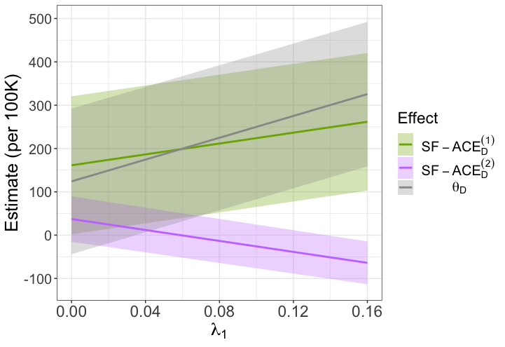
The S-Monotonicity assumption might be too restrictive, especially for the non-MSI-high subtype, for which there is limited information about the relative effect strength (Amitay et al. 2020). From a subject-manner perspective, we could not overlook the possibility of exposure-induced subtype switching for non-MSI-high subtype, as the relative effect of smoking on MSI-high CRC is known to be larger. Therefore, we replaced the S-Monotonicity assumption for non-MSI-high (subtype 1) with D-Monotonicity by fixing and varying the values of between 0 and (Figure 1). As increased, the estimated for non-MSI-high CRC increased, the estimated for MSI-high CRC decreased. For , was rejected. This result serves as evidence for heterogeneity in the as long as we believe subtype switching is possible and not extremely rare.
Given some a-priori evidence for smoking effects on both subtypes, we also considered an analysis under D-Monotonicity for both subtypes. Figure 2 presents the estimated effects on the difference scale as a function of and (for which the data did not restrict the range), along with 95% CIs. For nearly the entire range, the effect on non-MSI-high CRC was significant and the effect on MSI-high CRC was not. Sensitivity analysis results were similar for all three estimators (Figures 2, C.4 and C.5). As increased, the larger was the minimal value of for which heterogeneity can be concluded. For the RR (Figures C.6–C.8), under the combination of low and large the heterogeneity assumption was rejected.

As described in Section 2, there were 17,854 study participants for which the last available data were before age 70 (and they were not diagnosed with CRC and did not die). We treated these people as CRC-free at age 70. To assess the impact of this decision, we repeated our analyses while removing these people. In an additional analysis, we again removed these people but used inverse probability of weighting to take them into account. The results did not change materially, although the estimated effect sizes and the standard errors were generally larger (Tables C.13 and C.14).
To summarize our main findings, we have provided evidence for smoking effect on both CRC MSI subtypes and evidence for heterogeneity under reasonable causal assumptions. Even though our case numbers were smaller and our follow-up was more limited than previous studies, the estimated lend support of a causal effect on non-MSI-high CRC, for which available evidence was limited.
8 Discussion
Questions of etiologic heterogeneity are central to our understanding of how diseases evolve. Viewed through the lenses of competing events, existing approaches largely overlooked formal discussions of causal estimands and identifiability assumptions. On the other hand, the recent progress in causal inference methodology for competing events presented causal estimands that either provide little information about etiology heterogeneity or estimands requiring identifiability assumptions that are implausible in the study of CRC subtypes.
In this paper, to study the effect of smoking on CRC subtypes defined by MSI status, we proposed the SF-ACEs as causal effects that can complement existing methods and provide further insight towards the study of etiologic heterogeneity. One challenge with using multinomial regression with cohort data is the issue of right censoring due to loss to follow-up or administrative censoring. To assess its impact, we considered in this paper a number of analyses. The censoring problem would have been more pronounced if follow-up was longer than 10 years. Therefore, considering time-to-event outcomes is an important topic of future research. Another potential extension will consider continuous exposures instead of binary ones. Specifically, the generalization of the monotonicity assumptions, both in terms of definition and plausibility, is of interest.
References
- Amitay et al. (2020) Amitay, E. L., P. R. Carr, L. Jansen, W. Roth, E. Alwers, E. Herpel, M. Kloor, H. Bläker, J. Chang-Claude, H. Brenner, and M. Hoffmeister (2020). Smoking, alcohol consumption and colorectal cancer risk by molecular pathological subtypes and pathways. British Journal of Cancer 122(11), 1604–1610.
- Bang and Robins (2005) Bang, H. and J. M. Robins (2005). Doubly robust estimation in missing data and causal inference models. Biometrics 61(4), 962–973.
- Begg et al. (2018) Begg, C. B., V. E. Seshan, and E. C. Zabor (2018). Re:“a multinomial regression approach to model outcome heterogeneity”. American journal of epidemiology 187(5), 1129–1130.
- Carr et al. (2018) Carr, P., E. Alwers, S. Bienert, J. Weberpals, M. Kloor, H. Brenner, and M. Hoffmeister (2018). Lifestyle factors and risk of sporadic colorectal cancer by microsatellite instability status: a systematic review and meta-analyses. Annals of Oncology 29(4), 825–834.
- Chatterjee (2004) Chatterjee, N. (2004). A two-stage regression model for epidemiological studies with multivariate disease classification data. Journal of the American Statistical Association 99(465), 127–138.
- Frangakis and Rubin (2002) Frangakis, C. E. and D. B. Rubin (2002). Principal stratification in causal inference. Biometrics 58(1), 21–29.
- Hernán and Robins (2020) Hernán, M. A. and J. M. Robins (2020). Causal inference: what if. Boca Raton: Chapman & Hill/CRC 2020.
- Liu et al. (2018) Liu, L., D. Nevo, R. Nishihara, Y. Cao, M. Song, T. S. Twombly, A. T. Chan, E. L. Giovannucci, T. J. VanderWeele, M. Wang, and S. Ogino (2018). Utility of inverse probability weighting in molecular pathological epidemiology. European journal of epidemiology 33(4), 381–392.
- Lunceford and Davidian (2004) Lunceford, J. K. and M. Davidian (2004). Stratification and weighting via the propensity score in estimation of causal treatment effects: a comparative study. Statistics in medicine 23(19), 2937–2960.
- Nevo et al. (2018) Nevo, D., R. Nishihara, S. Ogino, and M. Wang (2018). The competing risks cox model with auxiliary case covariates under weaker missing-at-random cause of failure. Lifetime data analysis 24(3), 425–442.
- Nevo et al. (2021) Nevo, D., S. Ogino, and M. Wang (2021). Reflection on modern methods: causal inference considerations for heterogeneous disease etiology. International Journal of Epidemiology.
- Nevo et al. (2016) Nevo, D., D. M. Zucker, R. M. Tamimi, and M. Wang (2016). Accounting for measurement error in biomarker data and misclassification of subtypes in the analysis of tumor data. Statistics in medicine 35(30), 5686–5700.
- Ogino et al. (2016) Ogino, S., R. Nishihara, T. J. VanderWeele, M. Wang, A. Nishi, P. Lochhead, Z. R. Qian, X. Zhang, K. Wu, H. Nan, et al. (2016). The role of molecular pathological epidemiology in the study of neoplastic and non-neoplastic diseases in the era of precision medicine. Epidemiology (Cambridge, Mass.) 27(4), 602.
- Robins (1986) Robins, J. (1986). A new approach to causal inference in mortality studies with a sustained exposure period—application to control of the healthy worker survivor effect. Mathematical modelling 7(9-12), 1393–1512.
- Robins et al. (1994) Robins, J. M., A. Rotnitzky, and L. P. Zhao (1994). Estimation of regression coefficients when some regressors are not always observed. Journal of the American statistical Association 89(427), 846–866.
- Rubin (2006) Rubin, D. B. (2006). Causal inference through potential outcomes and principal stratification: application to studies with “censoring” due to death. Statistical Science 21(3), 299–309.
- Stensrud et al. (2020) Stensrud, M. J., J. G. Young, V. Didelez, J. M. Robins, and M. A. Hernán (2020). Separable effects for causal inference in the presence of competing events. Journal of the American Statistical Association, 1–9.
- Sun et al. (2017) Sun, B., T. VanderWeele, and E. J. Tchetgen Tchetgen (2017). A multinomial regression approach to model outcome heterogeneity. American journal of epidemiology 186(9), 1097–1103.
- Sun et al. (2018) Sun, B., T. VanderWeele, and E. J. Tchetgen Tchetgen (2018, 03). THE AUTHORS REPLY. American Journal of Epidemiology 187(5), 1130–1131.
- Ugai et al. (2022) Ugai, T., J. P. Väyrynen, K. Haruki, N. Akimoto, M. C. Lau, R. Zhong, J. Kishikawa, S. A. Väyrynen, M. Zhao, K. Fujiyoshi, et al. (2022). Smoking and incidence of colorectal cancer subclassified by tumor-associated macrophage infiltrates. JNCI: Journal of the National Cancer Institute 114(1), 68–77.
- Wang et al. (2015) Wang, M., A. Kuchiba, and S. Ogino (2015). A meta-regression method for studying etiological heterogeneity across disease subtypes classified by multiple biomarkers. American journal of epidemiology 182(3), 263–270.
- Wang et al. (2016) Wang, M., D. Spiegelman, A. Kuchiba, P. Lochhead, S. Kim, A. T. Chan, E. M. Poole, R. Tamimi, S. S. Tworoger, E. Giovannucci, et al. (2016). Statistical methods for studying disease subtype heterogeneity. Statistics in medicine 35(5), 782–800.
- Young et al. (2020) Young, J. G., M. J. Stensrud, E. J. Tchetgen Tchetgen, and M. A. Hernán (2020). A causal framework for classical statistical estimands in failure-time settings with competing events. Statistics in Medicine 39(8), 1199–1236.
- Zabor and Begg (2017) Zabor, E. C. and C. B. Begg (2017). A comparison of statistical methods for the study of etiologic heterogeneity. Statistics in medicine 36(25), 4050–4060.
- Zehavi and Nevo (2021) Zehavi, T. and D. Nevo (2021). A matching framework for truncation by death problems. arXiv preprint arXiv:2110.10186.
- Zhang and Rubin (2003) Zhang, J. L. and D. B. Rubin (2003). Estimation of causal effects via principal stratification when some outcomes are truncated by “death”. Journal of Educational and Behavioral Statistics 28(4), 353–368.
Appendix
- •
Section A includes proofs and additional theory. Section A.1 presents the proofs of Propositions 1–3. Section A.2 illustrates the the connection between observed data and the potential outcomes. Section A.3 discuss identification results under weaker combination of assumptions. Section A.4 provides the complete expression for the DR estimator.
- •
Section B includes details on the simulations and presents the results. Section B.1 gives additional details about the data generating mechanism of the simulation. Section B.2 presents the details of three different simulation studies. Finally, Section B.3 presents tables and figures summarizing the different simulation results.
- •
Section C presents details on the data as well as additional analyses and results. Section C.1 includes descriptive information about the data used. Section C.2 gives additional information about the weights used for handling missing subtypes and about the models fitted for estimating effects. Finally, Section C.3 presents additional data analysis results.
Appendix A Proofs and additional theory
A.1 Proof of identification results
Before providing the identification formulas for the , we first show that the equals to the when defined on the RR scale under S-Monotonicity for both disease subtypes.
A.1.1 Equivalence of the and TE
A.1.2 Proof of Proposition 1
Starting from the definition of , we have
| (A.15) | ||||
| (A.16) |
Equality (A.15) follows from the S-Monotonicity assumption for subtype 2, and (A.16) is justified because the subtypes are mutually exclusive (first expression in the numerator) and by S-Monotonicity for subtype 1 (second expression in the numerator).
For the standardization-based identification formula, we continue by recalling that under positivity and weak ignorability, is identified by
for (Hernán and Robins 2020). With previously denoted by for and hence equals to for , we substitute these expressions in (A.16) to get
| (A.17) |
Alternatively, to get IPTW-based identification results, we may continue from (A.16) by recalling that under positivity and weak ignorability, is identified by (Hernán and Robins 2020). Substituting these expressions in (A.16), we get
| (A.18) |
The identification formulas for subtype 2 are analogous. Using standardization,
or using IPTW,
The difference between the effects is given by substituting the expressions above in
The RR-based measures (A.14) are identified under weak ignorability and positivity using standardization by
for , or using IPTW,
Finally, define to be the difference between the effects in the RR scale. So is given by
A.1.3 Proof of Proposition 2
Recall that and . We start with the effect on subtype 1.
| (A.19) | ||||
| (A.20) | ||||
| (A.21) |
In (A.19), the numerator follows from the fact the subtypes are mutually exclusive and the denominator is justified by the law of total probability. In (A.20), the numerator holds because of the law of total probability and the denominator follows by noting that the D-Monotonicity assumption for subtype 2 implies .
Now, similarly to the proof of Proposition 1, we can continue using standardization,
by weak ignorability and positivity. Alternatively, as in the proof of Proposition 1, we can continue from (A.21) using IPTW to obtain
again by weak ignorability and positivity, similarly to the standard IPTW-based identification.
The identification formulas for subtype 2 are analogous. Using standardization,
or using IPTW,
The difference between the effects is given by
A.1.4 Proof of Proposition 3
Recall that and . We start with the effect on subtype 1.
| (A.22) | ||||
| (A.23) | ||||
Equality (A.22) holds because the subtypes are mutually exclusive. Equality (A.23) is by the law of total probability. As before, using standardization, we may write
or using IPTW,
The identification formula of subtype 2 is analogous. Using standardization,
or using IPTW,
The difference between the effects is given by .
An interesting distinction between the results in Propositions 2 and 3 compared to Proposition 1, is that if one further assumes S-Monotonicity for one of the subtypes only, such that S-Monotonicity holds for one subtype only, say subtype 1 so , then the identification formulas for the two subtypes are no longer symmetric.
A.2 Relationship between observed data and potential outcome profiles
Table 1 of the main text defines the nine possible potential outcome profiles. Table A.3 specifies the possible profiles for each participant according to their observed data under each of the four combinations of assumptions.
Observed data Monotonicity assumptions S-Mono S-Mono D-Mono D-Mono S-Mono D-Mono D-Mono S-Mono 0,1,3 0,1,3 0,1,3 0,1,3 5 5,7 5 5,7 6 6,8 6,8 6 0 0 0 0 3, 5 3, 5,8 3,5,8 3, 5 1, 6 1,6,7 1,6 1,6,7
A.3 Additional identification results
A.3.1 S-Monotonicity for one subtype and no monotonicity assumption for the other subtype
We present here identification for the under S-Monotonicity for subtype 1 and no monotonicity assumption, of any version, for subtype 2. To this end, in addition to , we define an additional sensitivity parameter . This sensitivity parameter is the probability to be CRC-free when exposed among those who would have been diagnosed with subtype 2 had they were unexposed. Under either S-Monotonicity or D-Monotonicity, .
We begin with the effect on subtype 1,
| (A.24) | ||||
| (A.25) | ||||
| (A.26) | ||||
Equality (A.24) holds because the subtypes are mutually exclusive and because of the equality which holds due to the S-Monotonicity assumption for subtype 1. Equality (A.25) holds because of the law of total probability. Equality (A.26) holds because of the law of total probability and because the subtypes are mutually exclusive.
Because different assumptions were made for subtype 1 and subtype 2, the effects are not analogous. Turning to the effect on subtype 2,
| (A.27) | ||||
| (A.28) | ||||
| (A.29) | ||||
Equality (A.27) holds because of the S-Monotonicity assumption for subtype 1. Equality (A.28) holds because the subtypes are mutually exclusive. Equality (A.29) holds because of the law of total probability. As before, standardization, IPTW or DR estimation can be used to identify and estimate the effects.
A.3.2 Sensitivity analysis without monotonicity assumptions
We present here identification on the difference scale, for the under no specified monotonicity assumptions for both subtypes. Recall that , and .
We begin with the effect on subtype 1,
| (A.30) | ||||
| (A.31) | ||||
| (A.32) | ||||
Equality (A.30) holds because the subtypes are mutually exclusive. Equality (A.31) holds because of the law of total probability. Equality (A.32) holds because of the law of total probability and because the subtypes are mutually exclusive.
The identification formula of subtype 2 is analogous, and requires one additional parameter .
As before, standardization, IPTW or DR estimation can be used to identify and estimate the effects.
A.4 Details about the doubly-robust estimator
Appendix B Additional simulation details and results
Section B.1 gives additional details about the data generating mechanism of the simulation. Section B.2 presents the details of three different simulation studies. Finally, Section B.3 presents tables and figures summarizing the different simulation results.
B.1 Data generating mechanism
The data were simulated to resemble an observational study. For each individual , we first simulated two independent measured confounders, , where and and one normally distributed unmeasured covariate . To simulate the potential outcomes, we used the multinomial regression model
| (A.33) |
for , and
We first simulated the potential outcome under no exposure , for each individual , using model (A.33). To make sure the data followed the S-Monotonicity assumption for both disease subtypes, the potential outcomes under exposure () were created as follows: Individuals with , namely that they would have been diagnosed with disease subtype 1 or 2 under , would automatically be diagnosed with the same disease subtype under . For individuals who were disease-free under the disease subtype under was simulated using Equation (A.33) with an adjusted probability using the Law of Total Probability,
We simulated the actual exposure status for each individual using a logistic regression model,
| (A.34) |
The observed outcome was obtained for each individual by setting s. For each individual , the observed data were ().
B.2 Additional details about the simulation studies
As indicated in the main text, in each of the studies and scenarios described below, we first estimated using a multinomial regression model and using a logistic regression model. Then, we computed the estimators for the conditional statistical estimand, the total effect, and the three estimators.
Three studies were investigated. In Study I, we fixed the model parameters and varied the sample size between 5,000 and 50,000. In Study II, we varied , the effect of the unmeasured covariate on , while keeping all the other parameters fixed. In Study III, we investigated the estimators’ performance when the models fitted were misspecified. To achieve this, a transformation of was used to create the data, but the analysis assumed is (logit) linearly connected to the exposure or/and the outcome. Misspecification of the relationship was created by taking when generating the data instead of . Misspecification of the model was also created by replacing with when generating the data. Table B.4 gives the model parameters and sample sizes used in the three studies. It also gives the obtained true values for each set of parameters yields. In all studies, the prevalence of subtype 1 ranged between 5%-6% and the prevalence of subtype 2 ranged between 2%-4%. The prevalence of the exposure was 49%.
| Study | n | † | † | ||||||||||||
| I | 5,000 | (, ) | (, ) | (, ) | 3470.5 | 969.1 | 1.75 | 1.61 | |||||||
| 10,000 | (, ) | (, ) | (, ) | 3470.5 | 969.1 | 1.75 | 1.61 | ||||||||
| 25,000 | (, ) | (, ) | (, ) | 3470.5 | 969.1 | 1.75 | 1.61 | ||||||||
| 50,000 | (, ) | (, ) | (, ) | 3470.5 | 969.1 | 1.75 | 1.61 | ||||||||
| II | 10,000 | (, ) | (, ) | (, ) | 3470.5 | 969.1 | 1.75 | 1.61 | |||||||
| 10,000 | (, ) | (, ) | (, ) | 3417.6 | 1228.2 | 1.78 | 1.76 | ||||||||
| 10,000 | (, ) | (, ) | (, ) | 3364.5 | 1498.5 | 1.77 | 1.71 | ||||||||
| 10,000 | (, ) | (, ) | (, ) | 3320.2 | 1727.2 | 1.76 | 1.65 | ||||||||
| 10,000 | (, ) | (, ) | (, ) | 3261.1 | 1947.6 | 1.76 | 1.61 | ||||||||
| III | 10,000 | (, ) | (, ) | (, ) | 2406.1 to 3470.5 | 656.6 to 969.1 | 1.63 to 1.78 | 1.67 to 1.81 |
B.3 Simulation Results
Tables B.5 and B.6 present the result for Study I. As can be seen from the Tables, the estimators had a smaller relative bias than the other estimators, even with a small sample size. The SD of all estimators in each sample size was similar, and the bootstrap SE estimator was approximately unbiased. The Wald-type CIs for the estimators had a satisfactory empirical coverage level, close to the desired 95%.
| Subtype | Sample Size | Effect | Method | Diff | ||||
| Bias | %Bias | CP95 | emp.SD | est.SE | ||||
| subtype 1 | 5,000 | Stand | -18.3 | -0.5 | 94.6 | 694.6 | 703.0 | |
| IPTW | -26.2 | -0.8 | 94.8 | 711.1 | 718.1 | |||
| DR | -23.0 | -0.7 | 94.9 | 704.5 | 714.2 | |||
| Stand | -86.8 | -2.5 | 94.5 | 681.1 | 689.2 | |||
| Stand | 98.3 | 2.8 | 94.7 | 706.7 | 713.7 | |||
| 10,000 | Stand | 1.9 | 0.1 | 94.9 | 492.0 | 496.2 | ||
| IPTW | -3.0 | -0.1 | 94.9 | 502.5 | 507.4 | |||
| DR | -1.9 | -0.1 | 94.9 | 499.3 | 504.6 | |||
| Stand | -67.1 | -1.9 | 95.1 | 482.4 | 486.5 | |||
| Stand | 119.3 | 3.4 | 94.7 | 499.3 | 503.7 | |||
| 25,000 | Stand | 10.1 | 0.3 | 96.2 | 309.2 | 315.3 | ||
| IPTW | 4.1 | 0.1 | 95.5 | 320.9 | 322.5 | |||
| DR | 4.9 | 0.1 | 95.3 | 318.5 | 320.8 | |||
| Stand | -59.4 | -1.7 | 95.7 | 303.2 | 309.1 | |||
| Stand | 129.3 | 3.7 | 93.9 | 314.0 | 320.1 | |||
| 50,000 | Stand | 10.8 | -0.3 | 95.1 | 221.2 | 221.3 | ||
| IPTW | -14.1 | -0.4 | 95.2 | 225.0 | 226.1 | |||
| DR | -13.7 | -0.3 | 95.0 | 225.0 | 225.0 | |||
| Stand | -79.7 | -2.3 | 93.8 | 217.1 | 217.1 | |||
| Stand | 107.0 | 3.1 | 91.7 | 224.0 | 224.6 | |||
| subtype 2 | 5,000 | Stand | 6.3 | 0.6 | 94.4 | 393.4 | 393.0 | |
| IPTW | 6.4 | 0.7 | 94.5 | 404.9 | 402.2 | |||
| DR | 5.5 | 0.6 | 94.9 | 402.0 | 401.7 | |||
| Stand | -69.0 | -7.1 | 93.9 | 362.9 | 362.7 | |||
| Stand | 152.3 | 15.7 | 93.0 | 422.8 | 422.3 | |||
| 10,000 | Stand | 13.2 | 1.4 | 94.8 | 277.6 | 277.5 | ||
| IPTW | 12.7 | 1.3 | 94.6 | 286.0 | 285.2 | |||
| DR | 12.2 | 1.3 | 94.7 | 285.3 | 284.6 | |||
| Stand | -62.7 | -6.5 | 95.0 | 256.3 | 256.2 | |||
| Stand | 160.2 | 16.5 | 91.2 | 298.9 | 298.1 | |||
| 25,000 | Stand | 23.1 | 2.4 | 93.5 | 182.7 | 175.9 | ||
| IPTW | 20.5 | 2.1 | 94.6 | 188.4 | 181.4 | |||
| DR | 20.5 | 2.1 | 94.4 | 188.8 | 180.9 | |||
| Stand | -53.5 | -5.5 | 93.5 | 168.7 | 162.3 | |||
| Stand | 170.2 | 17.6 | 83.1 | 196.5 | 188.8 | |||
| 50,000 | Stand | 19.7 | 2.0 | 93.5 | 130.0 | 124.9 | ||
| IPTW | 17.4 | 1.8 | 93.5 | 135.4 | 128.4 | |||
| DR | 17.1 | 1.76 | 93.7 | 135.0 | 127.1 | |||
| Stand | -56.6 | -5.8 | 90.3 | 120.0 | 114.4 | |||
| Stand | 167.0 | 17.3 | 83.1 | 140.1 | 133.9 | |||
| RR | ||||
| Bias | %Bias | CP95 | emp.SD | est.SE |
| 0.01 | 0.60 | 94.50 | 0.22 | 0.23 |
| 0.01 | 0.56 | 94.40 | 0.23 | 0.24 |
| 0.01 | 0.59 | 94.70 | 0.23 | 0.23 |
| 0.01 | 0.60 | 94.50 | 0.22 | 0.23 |
| 0.03 | 1.52 | 94.80 | 0.23 | 0.23 |
| 0.01 | 0.42 | 95.20 | 0.16 | 0.16 |
| 0.01 | 0.35 | 95.70 | 0.16 | 0.16 |
| 0.01 | 0.36 | 95.40 | 0.16 | 0.16 |
| 0.01 | 0.42 | 95.20 | 0.16 | 0.16 |
| 0.02 | 1.36 | 95.20 | 0.16 | 0.16 |
| 0.01 | 0.29 | 95.20 | 0.10 | 0.10 |
| 0.00 | 0.13 | 94.70 | 0.10 | 0.10 |
| 0.00 | 0.15 | 94.80 | 0.10 | 0.10 |
| 0.01 | 0.29 | 95.20 | 0.10 | 0.10 |
| 0.02 | 1.25 | 95.70 | 0.10 | 0.10 |
| 0.00 | -0.19 | 94.80 | 0.07 | 0.07 |
| 0.01 | -0.29 | 95.60 | 0.07 | 0.07 |
| 0.01 | -0.29 | 95.20 | 0.07 | 0.07 |
| 0.00 | -0.19 | 94.80 | 0.07 | 0.07 |
| 0.01 | 0.75 | 94.50 | 0.07 | 0.07 |
| 0.11 | 6.26 | 95.70 | 0.54 | 5.55 |
| 0.13 | 7.15 | 95.70 | 0.59 | 5.56 |
| 0.13 | 7.00 | 96.50 | 0.59 | 5.55 |
| 0.11 | 6.26 | 95.70 | 0.54 | 5.55 |
| 0.19 | 10.61 | 96.50 | 0.57 | 5.55 |
| 0.07 | 4.02 | 96.20 | 0.37 | 0.39 |
| 0.08 | 4.47 | 96.10 | 0.39 | 0.41 |
| 0.08 | 4.40 | 96.10 | 0.39 | 0.41 |
| 0.07 | 4.02 | 96.20 | 0.37 | 0.39 |
| 0.15 | 8.33 | 97.80 | 0.38 | 0.40 |
| 0.05 | 2.83 | 95.20 | 0.23 | 0.23 |
| 0.05 | 2.74 | 95.30 | 0.25 | 0.24 |
| 0.05 | 2.74 | 95.00 | 0.25 | 0.24 |
| 0.05 | 2.83 | 95.20 | 0.23 | 0.23 |
| 0.13 | 7.01 | 95.10 | 0.24 | 0.24 |
| 0.04 | 2.15 | 94.50 | 0.17 | 0.16 |
| 0.04 | 2.07 | 93.80 | 0.18 | 0.17 |
| 0.04 | 2.03 | 94.60 | 0.17 | 0.17 |
| 0.04 | 2.15 | 94.50 | 0.17 | 0.16 |
| 0.11 | 6.39 | 91.50 | 0.17 | 0.17 |
| Sample Size | Effect | Method | Diff | ||||
| Bias | %Bias | CP95 | emp.SD | est.SE | |||
| 5,000 | Stand | -24.6 | -1.0 | 95.2 | 791.1 | 810.5 | |
| IPTW | -32.6 | -1.3 | 94.5 | 809.1 | 828.8 | ||
| DR | -28.5 | -1.1 | 94.7 | 802.9 | 825.5 | ||
| Stand | -17.7 | -0.7 | 95.1 | 771.5 | 790.2 | ||
| Stand | -54.0 | -2.2 | 95.3 | 790.5 | 808.8 | ||
| 10,000 | Stand | -11.3 | -0.5 | 95.4 | 570.2 | 573.5 | |
| IPTW | -15.7 | -0.6 | 95.3 | 583.8 | 587.3 | ||
| DR | -14.1 | -0.6 | 94.9 | 581.7 | 585.0 | ||
| Stand | -4.4 | -0.2 | 95.3 | 555.7 | 559.2 | ||
| Stand | -40.9 | -1.6 | 95.1 | 569.6 | 572.4 | ||
| 25,000 | Stand | -13.0 | -0.5 | 94.4 | 363.9 | 361.8 | |
| IPTW | -16.4 | -0.7 | 94.1 | 378.2 | 370.9 | ||
| DR | -15.6 | -0.6 | 94.6 | 376.0 | 369.4 | ||
| Stand | -5.9 | -0.2 | 94.2 | 354.4 | 352.8 | ||
| Stand | -40.9 | -1.6 | 94.2 | 362.9 | 361.0 | ||
| 50,000 | Stand | -30.4 | -1.2 | 94.1 | 259.1 | 255.8 | |
| IPTW | -31.5 | -1.3 | 94.7 | 264.4 | 261.1 | ||
| DR | -30.8 | -1.2 | 94.6 | 263.0 | 260.4 | ||
| Stand | -23.1 | -0.9 | 94.5 | 252.1 | 248.1 | ||
| Stand | -60.1 | -2.4 | 94.0 | 258.0 | 254.1 | ||
| RR | ||||
| Bias | %Bias | CP95 | emp.SD | est.SE |
| -0.10 | 374.86 | 97.10 | 0.58 | 0.68 |
| -0.12 | 436.64 | 97.10 | 0.63 | 0.74 |
| -0.12 | 424.36 | 97.30 | 0.63 | 0.74 |
| -0.10 | 374.86 | 97.10 | 0.58 | 0.68 |
| -0.17 | 602.76 | 97.40 | 0.59 | 0.70 |
| -0.07 | 238.18 | 96.60 | 0.41 | 0.42 |
| -0.07 | 272.83 | 96.50 | 0.43 | 0.45 |
| -0.07 | 267.64 | 96.60 | 0.43 | 0.45 |
| -0.07 | 238.18 | 96.60 | 0.41 | 0.42 |
| -0.13 | 462.35 | 97.30 | 0.41 | 0.43 |
| -0.05 | 168.16 | 95.40 | 0.26 | 0.25 |
| -0.05 | 172.42 | 95.20 | 0.27 | 0.26 |
| -0.05 | 171.47 | 95.30 | 0.27 | 0.26 |
| -0.05 | 168.16 | 95.40 | 0.26 | 0.25 |
| -0.10 | 382.06 | 95.20 | 0.26 | 0.25 |
| -0.04 | 154.71 | 94.70 | 0.18 | 0.17 |
| -0.04 | 155.81 | 94.90 | 0.19 | 0.18 |
| -0.04 | 153.37 | 94.80 | 0.19 | 0.18 |
| -0.04 | 154.71 | 94.70 | 0.18 | 0.17 |
| -0.10 | 373.38 | 93.30 | 0.18 | 0.18 |
Turning to Study II, Figures B.3 and B.4 presents the bias of the different estimators, relative to the true s and , and as a function of the strength of the effect of on . The absolute difference between non- estimators and the s on the difference scale increased (in absolute value) as increased and remained the similar on the RR scale (Figure B.3). As expected, because the data were simulated under S-Monotonicity for both subtypes the and coincide on the RR scale. The relative bias (Figure B.4) remained generally the same. As all three methods (standardization, IPTW, and DR estimation) were based on correctly-specified models, their finite sample bias was minimal.


Finally, Table B.7 presents results from Study III under four settings: (a) Both and are correctly specified, (b) The model is correctly-specified and model is misspecified, (c) The model is misspecified and model is correctly-specified, and (d) both models are misspecified. As expected the standardization-based estimator had minimal bias when was correctly specified, and was biased when the model was misspecified. The IPTW-based model had minimal bias whenever model was correctly specified and produced considerable bias when the model was misspecified. As expected the DR estimator was only biased when both models were misspecified and had minimal bias under scenarios (a), (b), and (c) described above.
Table B.7 also shows that the SE was well estimated by the bootstrap and that the Wald-type 95% confidence intervals had satisfactory coverage rate whenever the respective model was correctly-specified.
| Method | Bias | %Bias | CP95 | emp.SD | est.SE |
| Both models correct | |||||
| Stand | 1.88 | 0.1 | 94.9 | 492.0 | 496.2 |
| IPTW | -2.99 | -0.1 | 94.9 | 502.5 | 507.3 |
| DR | -1.91 | -0.1 | 94.9 | 499.3 | 504.6 |
| Model is misspecified | |||||
| Stand | -35.05 | -1.0 | 95.0 | 508.2 | 509.6 |
| IPTW | 557.64 | 16.1 | 81.1 | 510.3 | 516.1 |
| DR | -37.65 | -1.1 | 94.8 | 508.3 | 510.0 |
| Model is misspecified | |||||
| Stand | -182.67 | -7.6 | 91.6 | 419.5 | 406.9 |
| IPTW | -4.19 | -0.2 | 93.6 | 494.8 | 481.0 |
| DR | -4.56 | -0.2 | 93.9 | 489.2 | 476.0 |
| Both models misspecified | |||||
| Stand | 2344.12 | 97.4 | 0.2 | 451.9 | 473.3 |
| IPTW | 2344.82 | 97.5 | 0.2 | 450.8 | 473.7 |
| DR | 2338.78 | 97.2 | 0.2 | 451.3 | 473.9 |
| Method | Bias | %Bias | CP95 | emp.SD | est.SE |
| Both models correct | |||||
| Stand | 13.16 | 1.36 | 94.80 | 277.60 | 277.52 |
| IPTW | 12.68 | 1.31 | 94.60 | 285.99 | 285.18 |
| DR | 12.18 | 1.26 | 94.70 | 285.28 | 284.61 |
| Model is misspecified | |||||
| Stand | 24.18 | 2.49 | 94.70 | 276.21 | 274.79 |
| IPTW | 199.86 | 20.62 | 89.40 | 279.62 | 278.17 |
| DR | 23.02 | 2.38 | 95.00 | 275.89 | 275.13 |
| Model is misspecified | |||||
| Stand | -89.72 | -13.6 | 92.6 | 217.5 | 214.5 |
| IPTW | 9.47 | 1.4 | 94.8 | 250.1 | 250.2 |
| DR | 9.26 | 1.4 | 94.6 | 249.7 | 249.5 |
| Both models misspecified | |||||
| Stand | 659.26 | 100.4 | 21.2 | 247.2 | 243.5 |
| IPTW | 663.16 | 100.9 | 21.2 | 246.6 | 243.6 |
| DR | 656.57 | 99.9 | 21.6 | 246.9 | 243.9 |
Appendix C Details on the data analysis and additional results
Section C.1 presents details on the data as well as additional analyses and results. Section C.1 includes descriptive information about the data used. Section C.2 gives additional information about the weights used for handling missing subtypes and about the models fitted for estimating effects. Finally, Section C.3 presents additional data analysis results.
C.1 Additional information about the data
Table C.9 gives basic descriptive information about the different covariates used in our analyses.
| Total | CRC free | MSI-high | Non-MSI-high | Missing subtype | |
| n = 109,272 | n = 108,853 | n = 61 | n = 358 | n=542 | |
| Smoking | |||||
| No | 50840 (46.5%) | 50667 (46.5%) | 24 (39.3%) | 149 (41.6%) | 229 (42.3%) |
| Yes | 58432 (53.5%) | 58186 (53.5%) | 37 (60.7%) | 209 (58.4%) | 313 (57.7%) |
| Gender | |||||
| Men (HPFS) | 28801 (26.4%) | 28675 (26.3%) | 15 (24.6%) | 111 (31%) | 169 (31.2%) |
| Women (NHS) | 80471 (73.6%) | 80178 (73.7%) | 46 (75.4%) | 247 (69%) | 373 (68.8%) |
| Body mass index | |||||
| high | 14506 (13.3%) | 14440 (13.3%) | 9 (14.8%) | 57 (15.9%) | 97 (17.9%) |
| low | 56789 (52%) | 56607 (52%) | 26 (42.6%) | 156 (43.6%) | 253 (46.7%) |
| normal | 37977 (34.8%) | 37806 (34.7%) | 26 (42.6%) | 145 (40.5%) | 192 (35.4%) |
| Using aspirin regularly | |||||
| No | 71180 (65.1%) | 70898 (65.1%) | 43 (70.5%) | 239 (66.8%) | 371 (68.5%) |
| Yes | 38092 (34.9%) | 37955 (34.9%) | 18 (29.5%) | 119 (33.2%) | 171 (31.5%) |
| Family history of colorectal cancer | |||||
| No | 95990 (87.8%) | 95641 (87.9%) | 48 (78.7%) | 301 (84.1%) | 469 (86.5%) |
| Yes | 13282 (12.2%) | 13212 (12.1%) | 13 (21.3%) | 57 (15.9%) | 73 (13.5%) |
| History of endoscopy | |||||
| No | 67821 (62.1%) | 67511 (62%) | 41 (67.2%) | 269 (75.1%) | 410 (75.6%) |
| Yes | 41451 (37.9%) | 41342 (38%) | 20 (32.8%) | 89 (24.9%) | 132 (24.4%) |
| Alcohol intake, g/d | 7.4 (11.0) | 7.4 (11.0) | 6.7 (10.6) | 8.3 (12.5) | 9.0 (13.3) |
| Total calorie intake, () | 1762.4 (496.5) | 1762.4 (496.5) | 1695.2 (460.5) | 1767.9 (499.3) | 1748.9 (542.5) |
| Physical activity, METS-h/wk | 20.0 (18.7) | 20.0 (18.7) | 17.3 (14.2) | 18.7 (20.2) | 19.0 (16.2) |
C.2 Additional information about the models
To take into account the individuals diagnosed with CRC without having their MSI subtype identified, we used inverse probability weighting (Liu et al. 2018). We fitted a logistic regression model among the individuals diagnosed with CRC, the outcome being missing or available MSI subtype. The covriates included were tumor location (proximal colon, distal colon, rectum, missing) disease stage (stage I, stage II, stage III, stage IV, missing), tumor differentiation (well, moderate, poor, unspecified, missing), age of diagnosis, year of diagnosis (1976–1995, 1996–2000, 2001–2012) and family history of colorectal cancer (yes or no). The estimates and 95% CI of the model coefficients are given in Table C.10. After fitting the model, we removed the individuals who were diagnosed with CRC but their MSI subtype was missing, and used weights based on the inverse of the logistic regression predictions to adjust our sample. We truncated the weights at the 99% percentile to reduce variance. The distribution of the final weights used are given in Figure C.5.
| Covariate | Estimate | 95% CI |
| Gender | 0.31 | (0.04, 0.58) |
| Tumor location - missing | 2.19 | (3.61, 0.76) |
| Tumor location - proximal colon | 0.02 | (0.24, 0.29) |
| Tumor location - rectum | 0.18 | (0.51, 0.14) |
| Disease stage - II | 0.01 | (0.32, 0.33) |
| Disease stage - III | 0.05 | (0.39, 0.29) |
| Disease stage - IV | 0.49 | (0.87, 0.11) |
| Disease stage - missing | 1.50 | (1.96, 1.03) |
| Tumor differentiation - missing | 0.50 | (2.35, 1.35) |
| Tumor differentiation - poor | 0.06 | (0.26, 0.38) |
| Tumor differentiation - unspecified | 0.59 | (0.96, 0.21) |
| Tumor differentiation - well | 0.26 | (0.63, 0.11) |
| Age of diagnosis | 0.03 | (0.002, 0.06) |
| Year of diagnosis - 2001–2012 | 0.66 | (0.96, 0.37) |
| Year of diagnosis - 1976–1995 | 0.65 | (0.98, 0.33) |
| Family history of CRC | 0.17 | (0.15, 0.49) |
When estimating the using IPTW and DR estimators, we fitted a logistic regression model, predicting the probability of smoking by age 60 based on the baseline covariats. The summary of this model is given in Table C.12. Similarly, when estimating the and using standardization and DR estimators, we fitted a multinomial regression model, predicting the probability of having non-MSI-high CRC, MSI-high CRC or being CRC free by age 70, based on smoking status by age 60 and the baseline covariates. The summary of this model is given in Table C.11.
| Covariate | non-MSI-high | MSI-high | ||
| Estimated OR | 95%CI | Estimated OR | 95%CI | |
| Smoking | 1.19 | (1.06, 1.33) | 1.39∗∗ | (1.38, 1.41) |
| Gender (Men) | 1.25∗∗ | (1.08, 1.42) | 0.87∗∗ | (0.83, 0.92) |
| Body mass index (low) | 0.68∗∗ | (0.54, 0.83) | 0.81∗ | (0.61, 1.01) |
| Body mass index (normal) | 1.04 | (0.90, 1.19) | 1.20∗ | (1.00, 1.39) |
| Using aspirin regularly | 0.93 | (0.78, 1.08) | 0.86∗∗ | (0.84, 0.87) |
| Alcohol intake | 1.00 | (1.00, 1.01) | 1.00 | (0.98, 1.02) |
| Total calorie intake | 1.00 | (1.00, 1.00) | 1.00∗∗ | (1.00, 1.00) |
| Family history of CRC | 1.52∗∗ | (1.33, 1.71) | 1.89∗∗ | (1.89, 1.90) |
| History of endoscopy | 0.44∗∗ | (0.27, 0.61) | 0.81∗∗ | (0.80, 0.81) |
| Physical activity | 1.00 | (1.00, 1.00) | 0.99 | (0.98, 1.01) |
| Covariate | Estimated OR | 95%CI |
| Gender (Men) | 0.67∗∗ | (0.64, 0.71) |
| Body mass index (low) | 0.99 | (0.95, 1.02) |
| Body mass index (normal) | 1.04 | (1.00, 1.08) |
| Using aspirin regularly | 1.05∗∗ | (1.03, 1.08) |
| Alcohol intake | 1.05∗∗ | (1.05, 1.05) |
| Total calorie intake | 1.00∗∗ | (1.00, 1.00) |
| Family history of CRC | 1.00 | (0.96, 1.04) |
| History of endoscopy | 0.95∗∗ | (0.92, 0.98) |
| Physical activity | 1.00∗∗ | (1.00, 1.00) |

C.3 Additional results
Turning to the analysis results. First, we estimated the effects under S-Monotonicity for both disease subtypes. The results for the are given in Table 2 of the main text. Here, we give the results for the in Table C.13, and the results for in Table C.14.
We then continued to the analysis under D-Monotonicity for both disease subtypes. The results for the and using the DR estimator were given in Figures 2 and 3 of the main text. Figures C.6 and C.7 give the corresponding results for standardization and IPTW methods. Figures C.8, C.9 and C.10 give the results for the and using standardization, IPTW and DR estimators, respectively. While the range for was [0, 1], we only considered . For larger values the estimators and hence estimators became unreasonably large.
Additionally, we give the results under D-Monotonicity for one subtype and S-Monotonicity for the other. The results for the and under the more plausible scenario of D-Monotonicity for subtype 1 and S-Monotonicity for subtype 2 are given in Figure 2 of the main text. For completeness, Figure C.11 gives the results for the and under D-Monotonicity for subtype 2 and S-Monotonicity for subtype 1. Figure C.12 gives the results for and . The estimator was relatively stable while increased as a function of and decreased as a function of .
Finally, we present the results of an analysis after removing participants for which the last available data were before age 70, with and without inverse probability weighting to take them into account (Tables C.15 and C.16)
| Subtype | Effect | Method | Estimate | SE | 95%CI |
| non-MSI-high | Stand | 1.19 | 0.15 | [0.91, 1.48] | |
| IPTW | 1.21 | 0.14 | [0.93, 1.48] | ||
| DR | 1.26 | 0.14 | [0.98, 1.54] | ||
| Stand | 1.19 | 0.15 | [0.91, 1.48] | ||
| MSI-high | Stand | 1.39 | 0.49 | [0.43, 2.35] | |
| IPTW | 1.39 | 0.40 | [0.60, 2.27] | ||
| DR | 1.48 | 0.43 | [0.64, 2.32] | ||
| Stand | 1.39 | 0.54 | [0.32, 2.46] |
| Scale | Effect | Method | Estimate | SE | 95%CI |
| Diff | Stand | 97.3 | 89.6 | [-78.3, 273.2] | |
| IPTW | 106.8 | 86.8 | [-63.7, 276.1] | ||
| DR | 124.1 | 85.8 | [-44.0, 292.6] | ||
| Stand | 97.4 | 88.6 | [-76.2, 271.1] | ||
| RR | Stand | -0.19 | 0.44 | [-1.05, 0.67] | |
| IPTW | -0.18 | 0.47 | [-1.08 0.72] | ||
| DR | -0.22 | 0.46 | [-1.12, 0.68] | ||
| Stand | -0.19 | 0.44 | [-1.05, 0.67] |


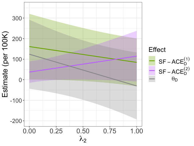

| Scale | Subtype | Effect | Method | Estimate | SE | 95%CI |
| Diff | non-MSI-high | Stand | 146.68 | 100.47 | [-50.24, 343.60] | |
| IPTW | 161.92 | 91.71 | [-17.82, 341.66] | |||
| DR | 186.87 | 105.60 | [-20.10, 393.83] | |||
| Stand | 146.48 | 91.81 | [-33.48, 326.43] | |||
| MSI-high | Stand | 37.98 | 28.58 | [-18.03, 93.99] | ||
| IPTW | 40.97 | 36.03 | [-29.64, 111.58] | |||
| DR | 44.01 | 30.45 | [-15.67, 103.69] | |||
| Stand | 37.62 | 30.49 | [-22.15, 97.38] | |||
| RR | non-MSI-high | Stand | 1.18 | 0.15 | [0.89, 1.47] | |
| IPTW | 1.21 | 0.15 | [0.92, 1.49] | |||
| DR | 1.25 | 0.13 | [0.99, 1.51] | |||
| Stand | 1.18 | 0.15 | [0.88, 1.48] | |||
| MSI-high | Stand | 1.38 | 0.39 | [0.60, 2.15] | ||
| IPTW | 1.43 | 0.42 | [0.61, 2.25] | |||
| DR | 1.48 | 0.58 | [0.35, 2.61] | |||
| Stand | 1.38 | 0.43 | [0.54, 2.22] |
| Scale | Subtype | Effect | Method | Estimate | SE | 95%CI |
| Diff | non-MSI-high | Stand | 130.66 | 98.68 | [-62.75, 324.07] | |
| IPTW | 145.93 | 91.88 | [-34.16, 326.02] | |||
| DR | 171.47 | 105.58 | [-35.45, 378.40] | |||
| Stand | 130.48 | 94.42 | [-54.58, 315.54] | |||
| MSI-high | Stand | 35.73 | 35.73 | [-34.31, 105.77] | ||
| IPTW | 38.75 | 35.93 | [-31.67, 109.17] | |||
| DR | 41.67 | 30.97 | [-19.03, 102.37] | |||
| Stand | 35.39 | 36.27 | [-35.70, 106.48] | |||
| RR | non-MSI-high | Stand | 1.16 | 0.15 | [0.87, 1.45] | |
| IPTW | 1.20 | 0.15 | [0.91, 1.48] | |||
| DR | 1.23 | 0.13 | [0.97, 1.48] | |||
| Stand | 1.16 | 0.15 | [0.87, 1.45] | |||
| MSI-high | Stand | 1.35 | 0.45 | [0.47, 2.23] | ||
| IPTW | 1.42 | 0.41 | [0.61, 2.23] | |||
| DR | 1.45 | 0.56 | [0.34, 2.55] | |||
| Stand | 1.35 | 0.55 | [0.27, 2.43] |