Concentration inequalities using approximate zero bias couplings with applications to Hoeffding’s statistic under the Ewens distributionThis research was partially supported by NSTDA young researcher fund 64000343.
Email: nathakhun.wir@kmutt.ac.th
Abstract
We prove concentration inequalities of the form for a random variable with mean zero and variance using a coupling technique from Stein’s method that is so-called approximate zero bias couplings. Applications to the Hoeffding’s statistic where the random permutation has the Ewens distribution with parameter are also presented. A few simulation experiments are then provided to visualize the tail probability of the Hoeffding’s statistic and our bounds. Based on the simulation results, our bounds work well especially when .
AMS 2010 subject classifications: Primary 60E15, 60C05 Secondary 62G10
Key words: Tail probabilities, Approximate Zero bias coupling, Stein’s method, Simulation, Accept-Reject algorithm, Ewens’s Sampling Formula
1 Introduction
Stein’s method was first introduced by Charles Stein in his seminal paper (Stein 1972) and is best known for obtaining non-asymptotic bounds on various distances for distributional approximations, see the text (Chen et al. 2011) and the introductory notes (Ross 2011). Thus far, many applications in several areas such as combinatorics, statistics, statistical physics and applied sciences have been developed using this method. Meanwhile, some researchers have used Stein’s method for non-distributional approximation contexts. Chatterjee 2007 introduced a version of Stein’s method for deriving concentration of measure inequalities.
The name ‘concentration of measure’ was first used in Talagrand 1995 when the author aimed to derive deviation bounds of the form in the situations where the exact evaluation is impossible or is hard to obtain. A bound of this form is considered ‘good’ if it decays sufficiently rapidly in . For instance, most of the works in the literature seek for bounds that are decreasing at exponential rate.
Now we only restrict our attention to concentration inequalities using Stein’s method. Laipaporn and Neammanee 2006 and Rattanawong 2013 obtained non-uniform concentration inequalities for randomized orthogonal array sampling designs and random permutation sum, respectively, however, they are not in the form that we focus on. Chatterjee 2007 used exchangeable pairs technique to provide concentration of measure for functions of dependent random variables, including the Hoeffding’s statistic when the random permutation has the uniform distribution and the net magnetization in the Curie-Weiss model. Once the connection between Stein’s method and concentration inequalities was uncovered, many results have been obtained using various techniques related to Stein’s method. Concentration bounds using bounded size bias couplings was introduced in Ghosh and Goldstein 2011b and Ghosh and Goldstein 2011a with examples including the number of relatively ordered subsequences of a random permutation, sliding window statistics, the lightbulb process, and etc. The same type of results with the help of bounded zero bias couplings occurred in Goldstein and Işlak 2014 with applications to the Hoeffding’s statistic where the random permutation has either the uniform distribution or one which is constant over permutations with the same cycle type and having no fixed points. The bounded size bias technique was strengthened in Arratia and Baxendale 2015 and the bounded assumption was relaxed by Cook et al. 2018 with applications to Erdös-Rényi graphs and permutation models.
In this work, we generalize the results in Goldstein and Işlak 2014 with zero bias couplings replaced by approximate zero bias couplings, first appeared in Wiroonsri 2017. This coupling is constructed by adding a remainder term to the construction of the zero bias coupling generated by a -Stein pair (see Goldstein and Reinert 1997 or Section 4.4 of Chen et al. 2011). Here we provide brief detail, presented in Wiroonsri 2017, of the construction of approximate zero bias couplings generated by approximate -Stein pairs. Recall that we call a pair of random variables , an approximate -Stein pair if it is exchangeable and satisfies
| (1) |
with , and
| (2) |
for some and .
Now we state the following lemma proved in Wiroonsri 2017 which is the generalized version of the result in Goldstein and Reinert 1997 with a -Stein pair replaced by an approximate -Stein pair. We call that satisfies (3), an approximate -zero bias variable.
Lemma 1.1
Let be an approximate -Stein pair with distribution . Then when has distribution
and has a uniform distribution on , independent of , the variable satisfies
| (3) |
for all absolutely continuous functions .
The core idea of Stein’s method is based on the fact that a mean zero random variable is normal if and only if for all absolutely continuous function. Therefore if and can be closely coupled by using Lemma 1.1 satisfying (3) with some small remainder term then we expect that the behavior of , including the decay of its tail probabilities, may be simlar to that of the normal. Wiroonsri 2017 obtained and bounds between and the standard normal in term of the difference and the remainder term . Here we focus on the concentration bounds on the same setting.
We also apply our result to the Hoeffding’s statistic (Hoeffding 1951) where the random permutation has the Ewens distribution. That is, we study the distribution of
| (4) |
where is a given real matrix with components and has the Ewens distribution where denotes the symmetric group. We note that the distribution of is of interest as it has a connection to nonparametric tests in statistics. Wiroonsri 2017 has succeeded in providing and bounds of order between and the normal by constructing an approximate -zero bias coupling and deriving the bounds based on the coupling. In the present work, we follow the construction there and apply the following main results to obtain concentration inequalities.
We now state the main theorem and then add a remark comparing the results here to the ones in Goldstein and Işlak 2014.
Theorem 1.2
Let be a mean zero random variable with variance and moment generating function , and let have the approximate -zero bias distribution satisfying (3), with and . Let if and are negatively correlated for where is given differently for each bound below and otherwise and . Assume that and are finite.
- (a)
If for some and exists for all with , then for all
(5) The same upper bound holds for if when exists for all . If for some and exists for all with then for all
(6) with the same upper bound for if and exists in .
- (b)
If for some and exists at then for ,
(7) If then the same bound holds for the left tail when .
Part (b) shows that the respective asymptotic orders as of and of the bounds (5) and (6) can be improved to .
Remark 1.3
- 1.
If , then and are zero and therefore the bounds (5), (6) and (7) in Theorem 1.2 are exactly the same as (2), (3) and (4) of Goldstein and Işlak 2014, respectively. See Remark 2.1 of Goldstein and Işlak 2014 and a few paragraphs thereafter for a comparison to previous results in the literature.
- 2.
We note that the bounds in (5) and (6) will be effective only for , and the bound (7) for where is given in the statement of the theorem. Therefore the three bounds in Theorem 1.2 will be useful only if we can construct an approximate -Stein pair in such a way that or is in the range of the support of . Otherwise, the bounds will be trivial.
Stein’s method has been used with Ewens distribution recently in Gan and Ross 2021 where they obtained an upper bound on the total variabtion distance between the random partition generated by Ewens Sampling Formula and the Poisson-Dirichlet distribution. Ewens distribution has also attracted attention in other fields of mathematics for a while (see Johnson et al. 1997, Arratia et al. 2003, Crane 2016 and da Silva et al. 2020 for instance.)
The remainder of this work is organized as follows. We present an application to the Hoeffding’s statistic where the random permutation has the Ewens distribution in Section 2. A few simulation experiments are then performed in Section 3. Finally, we devote the last section for the proof of our main theorem.
2 The Hoeffding’s statistic under the Ewens measure
As introduced in the first section, we study the distribution of
| (8) |
where is a given real matrix with components and has the Ewens distribution. The original work (Hoeffding 1951) studied the asymptotic normality of when has a uniform distribution. We note that, in this section, we consider the symbols and interchageable with and , respectively.
We first briefly describe the Ewens distribution and state some important properties. The Ewens distribution on the symmetric group with parameter , was first introduced in Ewens 1972 and used in population genetics to describe the probabilities associated with the number of times that different alleles are observed in the sample; see also Arratia et al. 2003 for the description in mathematical context. Let . In the following, for and , we use the notations
For a permutation , the Ewens measure is given by
| (9) |
where denotes the number of cycles of . We note that specializes to the uniform distribution over all permutations when .
A permutation with the distribution can be constructed by the “so called” the Chinese restaurant process (see e.g. Aldous 1985 and Pitman 1996), as follows. For , is the unique permutation that maps to in . For , we construct from by either adding as a fixed point with probability , or by inserting uniformly into one of locations inside a cycle of , so each with probability . Following this construction, for where such that and , we have
| (10) |
A distribution on is said to be constant on cycle type if the probability of any permutation depends only on the cycle type where is the number of cycles of and we write for for simplicity. Concentration inequalities of where has either a uniform distribution or one which is constant over permutations with the same cycle type and having no fixed points were obtained in Goldstein and Işlak 2014 by using zero bias couplings. It follows from (9) directly that the Ewens distribution is constant on cycle type and allows fixed point. Due to the difference, the zero biasing technique does not work here and thus we use approximate zero biasing as discussed in the first section instead. We first follow the construction of approximate -zero bias couplings presented in Wiroonsri 2017 and then apply Theorem 1.2 to obtain concentration bounds. It is interesting to study the robustness and the sensitivity of the tail probabilities when the controlled assumptions have changed.
We begin with stating the definitions, notations and assumptions used in Wiroonsri 2017. Letting
| (11) |
by (10), we have
| (12) |
Letting
and using (12), we have
As a consequence, replacing by , we assume without loss of generality that
| (13) |
and for simplicity, we consider only the symmetric case, that is, for all . Also, to rule out trivial cases, we assume in what follows that . The explicit form of was calculated in Lemma 4.8 of Wiroonsri 2017 and as discussed in Remark 4.9 of Wiroonsri 2017, is of order when the elements of are well chosen so that they do not depend on and most of the elements are not the same number. In this case, there exists such that for .
The following theorem presents concentration inequalities for .
Theorem 2.1
Let and let be an array of real numbers satisfying
Let be a random permutation with the distribution , with . Then, with the sum in (8) and
the bounds in Theorem 1.2 hold with replaced by and .
Moreover,
where
| (14) |
and
| (15) |
In particular, if is chosen so that given in (16) and and are negatively correlated for , then
As mentioned earlier in Remark 1.3, the bounds arised in Theorem 2.1, are effective for where depends on the remainder term of the approximate -Stein pair and the bounds are trivial outside this range. Hence if is out of the support of , then the bound will not be useful. The best possible bound of that we can obtain in general is which depends on , nevertheless, it becomes which is of constant order in the case that and and are negatively correlated for .
To prove Theorem 2.1, we apply Theorem 1.2 from the introduction. That is, we have to construct an approximate -zero bias coupling from an approximate -Stein pair by using Lemma 1.1 in such a way that and are bounded and that . For this purpose, we state the following two lemmas. The first, Lemma 2.2 proved in Wiroonsri 2017, constructs an approximate -Stein pair for where is given by (8) with replacing . The bounds related to the remainder term are then obtained in Lemma 2.3. Below, for , we write if and are in the same cycle, let be the length of the cycle containing and let , be the permutation that transposes and .
Lemma 2.2 (Wiroonsri 2017)
For , let be an array of real numbers satisfying and where is as in (11). Let a random permutation has the Ewens measure with , and let be given by (8). Further, let be chosen independently of , uniformly from all pairs of distinct elements of . Then, letting and be given by (8) with replacing , is an approximate -Stein pair with
| (16) |
where
| (17) | |||||
Lemma 2.3
Proof: The bounds (19) of and (20) of were shown in Wiroonsri 2017. To prove (18), since , it suffices to bound in (17). For any fixed , using that and we have
and, if ,
Using that and that is maximized when , it follows that
Now we have all ingredients to prove Theorem 2.1.
Proof of Theorem 2.1: First we construct an approximate -Stein pair as in Lemma 2.2 with the remainder given in (16). Then, constructing an approximate -zero bias variable from the approximate Stein pair as in the proof of Theorem 4.1 of Wiroonsri 2017, we have . Invoking Theorem 1.2 with using the bounds of and in (18) and (20) of Lemma 2.3, respectively, completes the proof.
3 Simulation
In this section, we perform 4 simulation experiments. is generated by first randomly choosing from and equally and then letting and where is defined similarly to (11). We intentionally select such that for all with as defined in Theorem 1.2 so that the negative correlation assumption there is satisfied. To generate Ewens permutations with , we apply the accept-reject algorithm (see Robert and Casella 2013). Recall that the discrete version of the accept-reject algorithm is stated as follow.
Theorem 3.1 (Von Neumann 1951)
Let and be discrete random variables with probability mass functions and , respectively, where and have common support. Define
To generate a random variable :
- (a)
Generate Uniform, , independently.
- (b)
If , set ; otherwise, return to step (a).
In our case, and are with and uniform, respectively, with common support be all possible permutations . Recall that the probability mass functions of and are
where denotes the number of cycles of . It is easy to see that
3.1 Experiment 1
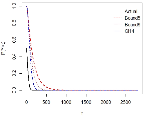
Let and . By simulating and for 1,000,000 times, we have , , , , support and from the sample. Figures 1 and 2 show for and the plot of compared with the bounds from (5) and (6), respectively. Note that we intend not to show (7) since at for large . Since is equivalent to the uniform distribution on , we also plot the bound from Goldstein and Işlak 2014. It is clear that the bound from Goldstein and Işlak 2014 is smaller as our coupling construction yields larger and that our bound is derived in a way to handle the remainder term so it is not as tight. However, the bound from Goldstein and Işlak 2014 does not work with .

3.2 Experiment 2
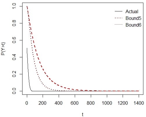
Since generating Ewens permutations with requires an algorithm, we are not able to generate a very big sample with large . Let and . implies that the chance of having a big number of cycles is less likely. By simulating and 10,000 times, we have , , , , support and from the sample. Figures 3 and 4 show for and the plot of compared with the bounds from (5) and (6), respectively. Note that the bound (7) is too large in this case because of the term .

3.3 Experiment 3
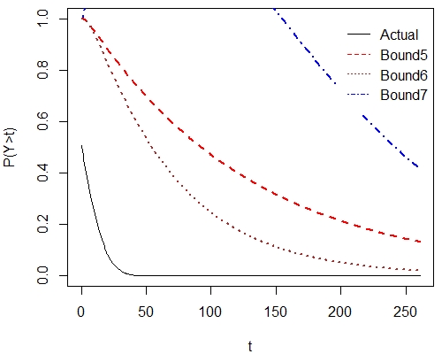
When increasing , it is more expensive to generate a permutation. Now we let and . provides that the chance of having a big number of cycles is more likely. By simulating and , 10,000 times, we have , , , , support and from the sample. Figures 5 and 6 show for and the plot of compared with the bounds from (5), (6) and (7), respectively.

3.4 Experiment 4
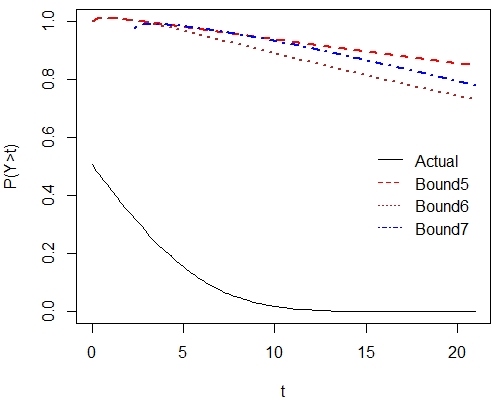
For this experiment, we intend to illustrate the case that is much greater than 1 which results in a permutation with much larger number of cycles. However, the simulation is very expensive which even takes 93.41 iterations on average to get only one permutation with and . Based on our simulation result with sample size of 10,000, the mean of the number of cycles is 4.03. By simulating and 10,000 times, we have , , , , support and from the sample. Figures 7 and 8 show for and the plot of compared with the bounds from (5), (6) and (7), respectively.

3.5 Conclusion from the simulation results
We can notice from the four experiments that our bounds seem to be more useful for smaller , especially when . For , the bounds are not sufficiently small even at the upper limit of the support. However, our experiments with are only done with small . Therefore, it is interesting to see whether our bounds will work better with larger .
4 Proof of the main result
In this section, we follow the same technique as in Goldstein and Işlak 2014 but handle a few extra terms that include .
Proof of Theorem 1.2: Let and . Using that , for we have
| (21) |
(a) If exists in an open interval containing we may interchange expectation and differentiation at to obtain
| (22) | |||||
where we have used the approximate zero bias relation in the second equality.
For and , using for we have
| (23) |
Using (22) and applying (23), we have
| (24) | |||||
Recalling from the statement of the theorem that if and and are negatively correlated for and otherwise and , it follows from the last expression that
Dividing both sides by , integrating over and using that yield
and therefore
We note that the claim for is clear as the right hand side of (5) is one. Applying Markov’s inequality for , we obtain
Letting that lies in , (5) holds. The result for the left tail when follows immediately from the same proof by letting and the fact that has the approximate -zero bias distribution with replaced by . We also note that the results for the left tail in the other cases below follow by the same argument so it suffices to prove only the results for the right tail.
Next we prove (6). Following the same argument as in Goldstein and Işlak 2014 and using that
for and , we have
Taking expectation and simplifying, we obtain
Using (24) and proceeding as in the first bound yield
We note that the claim for is clear as the right hand side of (6) is one. Again applying Markov’s inequality for , we have
Letting that lies in , (6) follows.
(b) For any such that exists, using (22), (21) and that if and and are negatively correlated for and otherwise and , we have
and thus
Integrating over we obtain
and hence
Again, by Markov’s inequality,
Now, for , choosing , we have
Using that for all yields the second inequality in (7).
References
- Aldous (1985) Aldous, D. J. (1985). Exchangeability and related topics. In École d’Été de Probabilités de Saint-Flour XIII—1983, pp. 1–198. Lecture Notes in Math., 1117, Springer, Berlin.
- Arratia et al. (2003) Arratia, R., A. D. Barbour, and S. Tavaré (2003). Logarithmic combinatorial structures: a probabilistic approach. European Mathematical Society.
- Arratia and Baxendale (2015) Arratia, R. and P. Baxendale (2015). Bounded size bias coupling: a gamma function bound, and universal dickman-function behavior. Probability Theory and Related Fields 162(3), 411–429.
- Chatterjee (2007) Chatterjee, S. (2007). Stein’s method for concentration inequalities. Probability theory and related fields 138(1-2), 305–321.
- Chen et al. (2011) Chen, L. H., L. Goldstein, and Q.-M. Shao (2011). Normal approximation by Stein’s method. Springer, New York.
- Cook et al. (2018) Cook, N., L. Goldstein, and T. Johnson (2018). Size biased couplings and the spectral gap for random regular graphs. The Annals of Probability 46(1), 72–125.
- Crane (2016) Crane, H. (2016). The ubiquitous Ewens sampling formula. Statistical science 31(1), 1–19.
- da Silva et al. (2020) da Silva, P. H., A. Jamshidpey, and S. Tavaré (2020). Random derangements and the Ewens sampling formula. arXiv preprint arXiv:2006.04840.
- Ewens (1972) Ewens, W. J. (1972). The sampling theory of selectively neutral alleles. Theoretical population biology 3(1), 87–112.
- Gan and Ross (2021) Gan, H. L. and N. Ross (2021). Stein’s method for the poisson–dirichlet distribution and the Ewens sampling formula, with applications to wright–fisher models. The Annals of Applied Probability 31(2), 625–667.
- Ghosh and Goldstein (2011a) Ghosh, S. and L. Goldstein (2011a). Applications of size biased couplings for concentration of measures. Electronic Communications in Probability 16, 70–83.
- Ghosh and Goldstein (2011b) Ghosh, S. and L. Goldstein (2011b). Concentration of measures via size-biased couplings. Probability theory and related fields 149(1), 271–278.
- Goldstein and Işlak (2014) Goldstein, L. and Ü. Işlak (2014). Concentration inequalities via zero bias couplings. Statistics & Probability Letters 86, 17–23.
- Goldstein and Reinert (1997) Goldstein, L. and G. Reinert (1997). Stein’s method and the zero bias transformation with application to simple random sampling. The Annals of Applied Probability 7(4), 935–952.
- Hoeffding (1951) Hoeffding, W. (1951). A combinatorial central limit theorem. Annals of Mathematical Statistics 22(4), 558–566.
- Johnson et al. (1997) Johnson, N. L., S. Kotz, and N. Balakrishnan (1997). Discrete multivariate distributions. Wiley, New York.
- Laipaporn and Neammanee (2006) Laipaporn, K. and K. Neammanee (2006). A non-uniform concentration inequality for randomized orthogonal array sampling designs. Thai Journal of Mathematics 4(1), 11–34.
- Pitman (1996) Pitman, J. (1996). Some developments of the blackwell-macqueen urn scheme. Lecture Notes-Monograph Series, 245–267.
- Rattanawong (2013) Rattanawong, P. (2013). A non-uniform concentration inequality for a random permutation sum. Communications in Statistics-Theory and Methods 42(10), 1879–1888.
- Robert and Casella (2013) Robert, C. and G. Casella (2013). Monte Carlo statistical methods. Springer Verlag, New York.
- Ross (2011) Ross, N. (2011). Fundamentals of Stein’s method. Probability Surveys 8, 210–293.
- Stein (1972) Stein, C. (1972). A bound for the error in the normal approximation to the distribution of a sum of dependent random variables. Proc. Sixth Berkeley Symp. Math. Statist. Prob. Univ. of California Press 2, 583–602.
- Talagrand (1995) Talagrand, M. (1995). Concentration of measure and isoperimetric inequalities in product spaces. Publications Mathématiques de l’Institut des Hautes Etudes Scientifiques 81(1), 73–205.
- Von Neumann (1951) Von Neumann, J. (1951). Various techniques in connection with random digits, collected works, volume v. Applied Math Series, Notes by G. E. Forsythe, in National Bureau of Standards 12, 36–38.
- Wiroonsri (2017) Wiroonsri, N. (2017). Stein’s method using approximate zero bias couplings with applications to combinatorial central limit theorems under the Ewens distribution. ALEA, Lat. Am. J. Probab. Math. Stat. 14, 917–946.