跳到论文正文
W Papers独立论文阅读器 arXiv:2206.00197 论文正文 计算阅读时间 · 0%
引用这篇论文根据当前论文元数据生成,正式投稿前建议核对。


License: CC BY 4.0
arXiv:2206.00197v1 [math.AP] 01 Jun 2022

Equilibria and energy minimizers for an interaction model on the hyperbolic space

Razvan C. Fetecau Thanks: Department of Mathematics, Simon Fraser University, 8888 University Dr., Burnaby, BC V5A 1S6, Canada; van@math.sfu.ca    Hansol Park Thanks: Department of Mathematics, Simon Fraser University, 8888 University Dr., Burnaby, BC V5A 1S6, Canada; hansol$_$park@sfu.ca
Abstract

We study an intrinsic model for collective behaviour on the hyperbolic space ℍn\mathbb{H}^{n}. We investigate the equilibria of the aggregation equation (or equivalently, the critical points of the associated interaction energy) for interaction potentials that include Newtonian repulsion. By using the method of moving planes, we establish the radial symmetry and the monotonicity of equilibria supported on geodesic balls of ℍn\mathbb{H}^{n}. We find several explicit forms of equilibria and show that one such equilibrium is a global energy minimizer. We also consider more general potentials and utilize a technique used for ℝn\mathbb{R}^{n} to establish the existence of compactly supported global minimizers. Numerical simulations are presented, suggesting that some of the equilibria studied here are global attractors. The key tool in our investigations is a family of isometries of ℍn\mathbb{H}^{n} that we have developed for this purpose.

Keywords: swarming on manifolds, hyperbolic space, energy minimizers, Newtonian potential

1 Introduction

In recent years there has been extensive work on investigating minimizers of nonlocal interaction energies, as motivated by a wide range of applications in a variety of disciplines, such as biology, physics, economics and social sciences [7, 16, 39, 2, 10, 24]. With very few exceptions, such works have studied the Euclidean case, where individual particles in ℝn\mathbb{R}^{n} interact via an interaction potential that depends on the Euclidean distance between them. Since our goal in this paper is to consider nonlocal interaction energies set up on Riemannian manifolds (in particular, on the hyperbolic space), we will present the general setup from the start.

Consider an nn-dimensional Riemannian manifold MM, and denote by 𝒫⁡(M)\mathcal{P}(M) the set of probability measures on MM. Define the interaction energy E:𝒫⁡(M)→ℝ∪{∞}E:\mathcal{P}(M)\to\mathbb{R}\cup\{\infty\} by

E⁡[ρ]=12​∬M×MK⁡(x,y)​𝑑ρ​(x)​𝑑ρ​(y),E[\rho]=\frac{1}{2}\iint_{M\times M}K(x,y)\mathrm{d}\rho(x)\mathrm{d}\rho(y), (1)

where K:M×M→ℝK:M\times M\to\mathbb{R} is an interaction potential that models attractive and repulsive interactions. More precisely, the negative manifold gradient −∇MK​(x,y)-\nabla_{M}K(x,y) (the gradient with respect to xx) of KK provides the interaction force that a point mass located at xx feels by interacting with a point mass located at yy [7, 23].

The interaction energy (1) is closely related to the following evolution equation for a population density ρ\rho:

∂tρ−∇M⋅(ρ​∇MK∗ρ)=0,\partial_{t}\rho-\nabla_{M}\cdot(\rho\nabla_{M}K\ast\rho)=0, (2)

where ∇M⋅\nabla_{M}\cdot denotes the manifold divergence on MM. Here, for a time-dependent measure ρt\rho_{t} on MM, the convolution K∗ρtK\ast\rho_{t} is defined by

K∗ρt​(x)=∫MK⁡(x,y)​d​ρt​(y).K*\rho_{t}(x)=\int_{M}K(x,y)\mathrm{d}\rho_{t}(y). (3)

Equation (2) is in the form of an active transport equation for the density ρ\rho, with a nonlocal velocity field given by

𝐯[ρ](x,t)=−∇MK∗ρt(x).\mathbf{v}[\rho](x,t)=-\nabla_{M}K*\rho_{t}(x). (4)

Note that 𝐯⁡[ρ]=−∇Mδ​E​[ρ]δ​ρ\displaystyle{\mathbf{v}[\rho]=-\nabla_{M}\frac{\delta E[\rho]}{\delta\rho}}, which sets (at least formally) equation (2) as the gradient flow of the energy (1). One can check by a direct calculation that indeed, formally, the energy EE decays in time along solutions of equation (2) [23]. Equilibria (steady states) of the aggregation model (2) are the critical points of the interaction energy, and from a dynamical point of view, we expect that solutions to model (2) approach asymptotically as t→∞t\to\infty, local minimizers of the energy.

There has been extensive literature in recent years on interaction energies of type (1), with the vast majority of the works focusing on the case M=ℝnM=\mathbb{R}^{n}. One approach is to use the techniques developed in [1] and formulate the gradient flow of the energy EE on the space of probability measures with finite second (or other order) moments, equipped with the 22-Wasserstein metric [13, 9, 41]. Another approach is to use direct methods of the calculus of variations and establish the existence of global minimizers (ground states) of the interaction energy [16, 39, 24]. There are also various studies of quantitative and qualitative properties of minimizers, such as their regularity [8] and compactness and dimensionality of their support [7, 2, 10].

Model (2) can exhibit a very diverse range of swarming or self-organized behaviour. We refer to [33, 40, 21, 3, 12] for explicit calculations and numerical illustrations of equilibria for the model in ℝn\mathbb{R}^{n}, which include aggregations on disks, annuli, rings, and soccer balls. The model on manifolds is far less investigated, but nevertheless, a similarly diverse set of equilibria was demonstrated in [23] for the hyperbolic plane and also, interesting aggregation patterns were shown in [19] for the model set up on the rotation group S​O​(3)SO(3). Applications of model (2) are numerous, e.g., to flocking and swarming of biological organisms [11], material science and granular media [13], self-assembly of nanoparticles [31], robotics [25, 32] and opinion formation [35].

In our study we will follow the intrinsic approach pursued in various recent papers [23, 19, 22] and assume that K⁡(x,y)K(x,y) only depends on the geodesic distance d⁡(x,y)d(x,y) between the two points. By an abuse of notation we write K⁡(x,y)=K⁡(d⁡(x,y))K(x,y)=K(d(x,y)). In contrast, when MM comes with a canonical embedding in a larger Euclidean space (e.g., a surface in ℝ3\mathbb{R}^{3}), K⁡(x,y)K(x,y) can be assumed to depend on the Euclidean distance |x−y||x-y| in the ambient space between xx and yy; we refer to this case as the extrinsic approach. The two approaches yield very different models (unless M=ℝnM=\mathbb{R}^{n}, in which case the two models are the same). For extrinsic models we refer to [41, 36] for studies on well-posedness by gradient flow techniques, and to various works on the emergent behaviours of the extrinsic models on manifolds, e.g., on sphere [15], unitary matrices [34, 30, 29], hyperbolic space [27], and Stiefel manifolds [28]. Relevant to the present paper, we note the work in [27], where the authors study synchronization behaviour on the hyperbolic space with an extrinsic quadratic potential (i.e., K⁡(x,y)=|x−y|2K(x,y)=|x-y|^{2}) for the discrete analogue of (2). A related study is done in [37]. The emergence of self-synchronization has been widely studied in the literature, due to its numerous occurrences in biological, physical and chemical systems (e.g., flashing of fireflies, neuronal synchronization in the brain, quantum synchronization) – see [34, 27] and references therein.

For intrinsic models, the sign of K′K^{\prime} determines whether the interactions are repulsive or attractive in nature. Indeed, provided xx and yy are not in the cut locus of each other, by chain rule one gets

−∇MK​(d⁡(x,y))=K′​(d⁡(x,y))​logx⁡yd⁡(x,y),-\nabla_{M}K(d(x,y))=K^{\prime}(d(x,y))\frac{\log_{x}y}{d(x,y)},

where logx⁡y\log_{x}y denotes the Riemannian logarithm map (i.e., the inverse of the Riemannian exponential map) on MM. Therefore, by interacting with the point mass at yy, the point mass at xx is driven by a force of magnitude proportional to |K′​(d​(x,y))||K^{\prime}(d(x,y))|, to move either towards yy (if K′​(d⁡(x,y))>0K^{\prime}(d(x,y))>0) or away from yy (if K′​(d⁡(x,y))<0K^{\prime}(d(x,y))<0). To obtain non-trivial swarming behaviours, repulsion and attraction must balance each other. Typically, such interaction potentials have short-range repulsion and long-range attraction, i.e., K′​(r)<0K^{\prime}(r)<0 for small rr and K′​(r)>0K^{\prime}(r)>0 for large rr (see Figure 2).

The interaction energy for intrinsic models is invariant under isometries. Indeed, if f:M→Mf:M\to M is an isometry of MM and f#​ρf_{\#}\rho is the push-forward by ff of the measure ρ\rho, then it is immediate to show that

E⁡[f#​ρ]=E⁡[ρ].E[f_{\#}\rho]=E[\rho]. (5)

Consequently, the energy minimizers can only be expected to be unique up to isometries.

In this paper we are exclusively concerned with studying the nonlocal aggregation model on the hyperbolic space ℍn\mathbb{H}^{n}, represented as a one-sheeted hyperboloid in ℝn+1\mathbb{R}^{n+1} endowed with the Lorentzian inner product. Based on the Lorentz transform, we construct a family of isometries of ℍn\mathbb{H}^{n} and a binary operation on ℍn×ℍn\mathbb{H}^{n}\times\mathbb{H}^{n}, along with a concept of coordinates on ℍn\mathbb{H}^{n}, that are the key tools in the results we establish in the present work.

In Section 3 we consider attractive-repulsive interaction potentials that include Newtonian repulsion, i.e., potentials for which the repulsion component is given by the Green’s function of the negative Laplacian on ℍn\mathbb{H}^{n}. We note here that the Green’s function on ℍn\mathbb{H}^{n} has an explicit expression [17] – see (28). For the model on ℝn\mathbb{R}^{n}, potentials in this form have been given extensive attention in recent years [6, 21, 20, 12, 38], and a potential with Newtonian repulsion was also considered on the hyperbolic plane [23]. In this section we only consider equilibria that are absolutely continuous with respect to the canonical volume measure on ℍn\mathbb{H}^{n}. This choice is motivated by results in the Euclidean space ℝn\mathbb{R}^{n} which have established that for interaction potentials with Newtonian repulsion, the local minimizers of the interaction energy are absolutely continuous with respect to the Lebegue measure [12].

We study equilibria supported in geodesic balls of ℍn\mathbb{H}^{n} and show that such equilibria must be radially symmetric and monotone with respect to the centre of the ball. To show this result (Theorem 3.3) we use the method of moving planes, a well-known method for studying qualitative properties of positive solutions of elliptic equations [26]. More recently, the method found applications in integral equations [14, 20]. The challenge here is to adapt the method to the hyperboloid; to the best of our knowledge this the first application of the method of moving planes to integral equations on manifolds. We also find several explicit forms of radially symmetric equilibria, corresponding to particular choices of the attractive part of the potential. For one such attractive potential, we show that the equilibrium we computed is in fact the global energy minimizer. We also present various numerical simulations in Section 5.

In Section 4 we investigate the existence of compactly supported global minimizers of the energy (1) for M=ℍnM=\mathbb{H}^{n}. As we apply and follow closely the technique used by Cañizo et al. [7] for the Euclidean case, we only highlight the main differences from their work. In other words, we are not aiming for a self-contained presentation in Section 4, as some of results from [7] would transfer with no modifications to ℍn\mathbb{H}^{n}. Nevertheless, we show how the family of isometries and the concept of coordinates on ℍn\mathbb{H}^{n} that we developed, enable a similar approach as for the Euclidean case. In particular, minimizers cannot have too large gaps, as otherwise, an isometric displacement of one of the components would decrease the energy (Lemma 4.3).

Finally, we provide some numerical results in Section 5. Using various interaction potentials, we illustrate the dynamical evolution to steady states of radially symmetric solutions to (2). The equilibria we present are qualitatively different in terms in their monotonicity, in consistency with the analytical findings. Numerics suggest these equilibria are global attractors for the dynamics (at least for radial initial densities).

The summary of the paper is the following. Section 2 provides key background needed for the paper, on the variational formalism and on the geometrical properties of ℍn\mathbb{H}^{n}. Section 3 contains analytical results for interaction potentials that contain Newtonian repulsion (characterization of monotonicity, explicit forms for equilibria, convexity of energy). In Section 4 we establish the existence of compactly supported global minimizers, following the approach for ℝn\mathbb{R}^{n} from [7]. Proof of various lemmas are deferred to the Appendix.

2 Preliminaries

In this section we provide some background on the variational formalism used in our paper, as well as on the various geometrical properties of ℍn\mathbb{H}^{n}, in particular on a family of isometries of the hyperbolic space that plays a key role in our studies.

2.1 Variational approach: Euler-Lagrange equations

For the interaction energy set up on the Euclidean space ℝn\mathbb{R}^{n}, there exists a well-established approach to characterize its local minimizers (by Euler-Lagrange equations) in the topology of transport distances [2]. As this approach extends immediately to arbitrary manifolds, we will simply list below the main notations and results.

Take pp to be a fixed point in MM, and denote by 𝒫2​(M)\mathcal{P}_{2}(M) the set of probability measures that have finite moments of order 22 (with respect to pp), i.e.,

𝒫2​(M)={μ∈𝒫⁡(M):∫Md2​(x,p)​𝑑μ​(x)<∞}.\mathcal{P}_{2}(M)=\left\{\mu\in\mathcal{P}(M):\int_{M}d^{2}(x,p)\mathrm{d}\mu(x)<\infty\right\}.

The 22-Wasserstein distance between two measures μ,σ∈𝒫2​(M)\mu,\sigma\in\mathcal{P}_{2}(M) is given by:

d22​(μ,σ)=infπ∈Π⁡(μ,σ)∬M×Md2​(x,y)​𝑑π​(x,y),d_{2}^{2}(\mu,\sigma)=\inf_{\pi\in\Pi(\mu,\sigma)}\iint_{M\times M}d^{2}(x,y)\mathrm{d}\pi(x,y),

where Π⁡(μ,σ)⊂𝒫⁡(M×M)\Pi(\mu,\sigma)\subset\mathcal{P}(M\times M) is the set of transport plans between μ\mu and σ\sigma, i.e., the set of probability measures on the product space M×MM\times M with first and second marginals μ\mu and σ\sigma, respectively.

A probability measure μ∈𝒫2​(M)\mu\in\mathcal{P}_{2}(M) is a local minimizer of EE with respect to the d2d_{2}-distance provided there exists ϵ>0\epsilon>0 such that E⁡[σ]≥E⁡[μ]E[\sigma]\geq E[\mu], for all σ∈B⁡(μ,ϵ)\sigma\in B(\mu,\epsilon), where B⁡(μ,ϵ)B(\mu,\epsilon) denotes the open ball (in d2d_{2}) centred at μ\mu and of radius ϵ\epsilon.

We will pay particular attention in this paper to probability measures that are absolutely continuous with respect to the canonical volume measure d​x\mathrm{d}x; we denote this space by 𝒫a​c​(M)\mathcal{P}^{ac}(M). Throughout the paper, we will refer to an absolutely continuous measure directly by its density ρ\rho, and by abuse of notation write ρ∈𝒫a​c​(M)\rho\in\mathcal{P}^{ac}(M) to mean d​ρ​(x)=ρ⁡(x)​d​x∈𝒫a​c​(M)\mathrm{d}\rho(x)=\rho(x)\mathrm{d}x\in\mathcal{P}^{ac}(M). Finally, we denote by 𝒫ca​c​(M)\mathcal{P}^{ac}_{c}(M) the space of absolutely continuous probability measures with compact support in MM.

The following result, stated originally for M=ℝnM=\mathbb{R}^{n}, extends trivially to arbitrary Riemannian manifolds.

Proposition 2.1 ([2], Theorem 4 and Remark 4).

Assume the interaction potential KK is bounded from below and lower semicontinuous. Let ρ∈𝒫a​c​(M)∩𝒫2​(M)\rho\in\mathcal{P}^{ac}(M)\cap\mathcal{P}_{2}(M) be a local minimizer of EE with respect to d2d_{2}. Then,

Λ⁡(x)\displaystyle\Lambda(x) =λ, for a.e. ​x∈supp⁡(ρ),\displaystyle=\lambda,\qquad\text{ for a.e. }x\in\mathrm{supp}(\rho), (6a)
Λ⁡(x)\displaystyle\Lambda(x) ≥λ, for a.e. on ​M∖supp⁡(ρ),\displaystyle\geq\lambda,\qquad\text{ for a.e. on }M\setminus\mathrm{supp}(\rho), (6b)

where

Λ⁡(x):=∫MK⁡(x,y)​ρ​(y)​𝑑y,\displaystyle\Lambda(x):=\int_{M}K(x,y)\rho(y)\mathrm{d}y, (7)

and λ=2​E​[ρ]\lambda=2E[\rho] is a constant.

Condition (6a) is shown by taking perturbations of ρ\rho supported in supp⁡(ρ)\mathrm{supp}(\rho). The condition is equivalent to ρ\rho being a critical point of EE, at which the first variation of the energy vanishes. The constant λ\lambda, which plays the role of a Lagrange multiplier in the derivation of (6a), has a physical interpretation [4]: it represents the energy per unit mass felt by a point mass at position xx due to interaction with all points in supp⁡(ρ)\mathrm{supp}(\rho).

We also note that critical points of the interaction energy represent equilibrium solutions (steady states) of the aggregation model (2). This can be inferred from the fact that the velocity 𝐯(x)=−∇MK∗ρ(x)=−∇MΛ(x)\mathbf{v}(x)=-\nabla_{M}K\ast\rho(x)=-\nabla_{M}\Lambda(x) vanishes for x∈supp⁡(ρ)x\in\mathrm{supp}(\rho), given that Λ\Lambda is constant in supp⁡(ρ)\mathrm{supp}(\rho). We will use these concepts (critical point of the energy, equilibrium solution, steady state) interchangeably in the sequel.

The necessary condition (6b) is found by taking perturbations of ρ\rho that can be supported anywhere in MM, in particular outside supp⁡(ρ)\mathrm{supp}(\rho). The interpretation of (6b) is that transporting mass from the support of ρ\rho into its complement increases the total energy (hence ρ\rho is a local minimizer, being in a favourably energetic state).

2.2 Geometric properties of the hyperbolic space ℍn\mathbb{H}^{n}

In this part, we present some geometric properties of the hyperbolic space ℍn\mathbb{H}^{n} which will be used in the paper.

2.2.1 Hyperboloid model, polar coordinates and notations

We consider the space ℝn+1\mathbb{R}^{n+1} endowed with the (negative) Lorentzian inner product:

⟨x,y⟩=x0​y0−x1​y1−⋯−xn​yn,\langle x,y\rangle=x_{0}y_{0}-x_{1}y_{1}-\cdots-x_{n}y_{n}, (8)

where x=(x0,x1,…,xn)x=(x_{0},x_{1},\dots,x_{n}), y=(y0,y1,…,yn)∈ℝn+1y=(y_{0},y_{1},\dots,y_{n})\in\mathbb{R}^{n+1}. The inner product (8) induces the (complex-valued) norm defined by

‖x‖=⟨x,x⟩12, for ​x∈ℝn+1.\|x\|=\langle x,x\rangle^{\frac{1}{2}},\qquad\text{ for }x\in\mathbb{R}^{n+1}. (9)

We use the hyperboloid model of the hyperbolic space and take:

ℍn:={x∈ℝn+1:−x02+x12+⋯+xn2=−1,x0>0}⊂ℝn+1,\mathbb{H}^{n}:=\{x\in\mathbb{R}^{n+1}:-x_{0}^{2}+x_{1}^{2}+\dots+x_{n}^{2}=-1,x_{0}>0\}\subset\mathbb{R}^{n+1},

or, written differently,

ℍn={x∈ℝn+1:x⊤ηx=−1,x0>0},\mathbb{H}^{n}=\{x\in\mathbb{R}^{n+1}:x^{\top}\eta x=-1,x_{0}>0\},

where η=diag⁡(−1,1,1,⋯,1⏟n−times)\eta=\mathrm{diag}(-1,\underbrace{1,1,\cdots,1}_{n-\text{times}}) is a matrix of size (n+1)×(n+1)(n+1)\times(n+1).

The geodesic distance d⁡(x,y)d(x,y) on ℍn\mathbb{H}^{n} between two points xx and yy, is given by:

d⁡(x,y)=cosh−1⁡(⟨x,y⟩)=cosh−1⁡(x0​y0−x1​y1−⋯−xn​yn).d(x,y)=\cosh^{-1}(\langle x,y\rangle)=\cosh^{-1}(x_{0}y_{0}-x_{1}y_{1}-\cdots-x_{n}y_{n}). (10)

For x∈ℍnx\in\mathbb{H}^{n} and R>0R>0, we denote by BR​(x)B_{R}(x) the open geodesic ball in ℍn\mathbb{H}^{n} centred at xx of radius RR, i.e.,

BR​(x)={y∈ℍn:d⁡(x,y)<R}.B_{R}(x)=\{y\in\mathbb{H}^{n}:d(x,y)<R\}.

We use the hyperbolic polar coordinates on ℍn\mathbb{H}^{n}, given by:

(θ,ξ)∈[0,∞)×𝕊n−1↦(cosh⁡θ,sinh⁡θ​ξ)∈ℍn⊂ℝn+1,\displaystyle(\theta,\xi)\in[0,\infty)\times\mathbb{S}^{n-1}\mapsto(\cosh\theta,\sinh\theta\,\xi)\in\mathbb{H}^{n}\subset\mathbb{R}^{n+1}, (11)

where 𝕊n−1\mathbb{S}^{n-1} denotes the (n−1)(n-1)-dimensional unit sphere embedded in ℝn\mathbb{R}^{n}. We denote by vv the vertex of ℍn\mathbb{H}^{n}, corresponding to θ=0\theta=0, i.e., v=(1,0,…,0)∈ℝn+1v=(1,0,\dots,0)\in\mathbb{R}^{n+1}. The vertex vv plays the role of the origin in the Euclidean space.

In polar coordinates, the Laplace-Beltrami operator Δℍn\Delta_{\mathbb{H}^{n}} can be written as:

Δℍn​f​(θ,ξ)=sinh1−n⁡θ​∂θ(sinhn−1⁡θ​∂θf)+sinh−2⁡θ​Δξ​f=∂θ​θf+(n−1)​coth⁡θ​∂θf+sinh−2⁡θ​Δξ​f,\displaystyle\begin{aligned} \Delta_{\mathbb{H}^{n}}f(\theta,\xi)&=\sinh^{1-n}\theta\,\partial_{\theta}\left(\sinh^{n-1}\theta\partial_{\theta}f\right)+\sinh^{-2}\theta\Delta_{\xi}f\\ &=\partial_{\theta\theta}f+(n-1)\coth\theta\,\partial_{\theta}f+\sinh^{-2}\theta\Delta_{\xi}f,\end{aligned} (12)

where Δξ\Delta_{\xi} is the Laplace–Beltrami operator on 𝕊n−1\mathbb{S}^{n-1}, with respect to the variable ξ\xi. Also, the canonical volume form on ℍn\mathbb{H}^{n} in these coordinates is given by

d​x=sinhn−1⁡θ​d​θ​d​σξ.\mathrm{d}x=\sinh^{n-1}\theta\,\mathrm{d}\theta\mathrm{d}\sigma_{\xi}. (13)

We denote by α⁡(n)\alpha(n) the volume of the nn-dimensional unit ball in ℝn\mathbb{R}^{n}; consequently, n​α​(n)n\alpha(n) is the surface area of 𝕊n−1\mathbb{S}^{n-1} in ℝn\mathbb{R}^{n}. Finally, we denote the standard Euclidean norm in ℝn\mathbb{R}^{n} by |⋅||\cdot|, i.e.,

|w|=(w12+⋯+wn2)12, for ​w=(w1,…,wn)∈ℝn.|w|=\left(w_{1}^{2}+\cdots+w_{n}^{2}\right)^{\frac{1}{2}},\qquad\text{ for }w=(w_{1},\dots,w_{n})\in\mathbb{R}^{n}.

2.2.2 Lorentz transform

For a fixed vector w=(w1,…,wn)∈ℝnw=(w_{1},\dots,w_{n})\in\mathbb{R}^{n} with |w|<1|w|<1, consider the following matrix B⁡(w)B(w) of size (n+1)×(n+1)(n+1)\times(n+1) with indices 0,1,…,n0,1,\dots,n:

B(w)00=γ,B(w)i​0=B(w)0​i=−γwi,B(w)i​j=δi​j+(γ−1)wi​wj|w|2,∀i,j=1,2,⋯,n,\displaystyle B(w)_{00}=\gamma,\quad B(w)_{i0}=B(w)_{0i}=-\gamma w_{i},\quad B(w)_{ij}=\delta_{ij}+(\gamma-1)\frac{w_{i}w_{j}}{|w|^{2}},\quad\forall i,j=1,2,\cdots,n, (14)

where γ=(1−|w|2)−1/2\gamma=(1-|w|^{2})^{-1/2}. Equivalently, the matrix expression of B⁡(w)B(w) is

B⁡(w)=[γ−γ​w⊤−γ​wIn+(γ−1)​w​w⊤|w|2].B(w)=\begin{bmatrix}\gamma&-\gamma w^{\top}\\ -\gamma w&I_{n}+(\gamma-1)\frac{ww^{\top}}{|w|^{2}}\end{bmatrix}.

We denote this matrix by BB, since the corresponding concept is the Lorentz boost.

Lemma 2.2.

For a fixed w∈ℝnw\in\mathbb{R}^{n} with |w|<1|w|<1, B⁡(w)B(w) maps ℍn\mathbb{H}^{n} into ℍn\mathbb{H}^{n}, i.e.,

y=B⁡(w)​x∈ℍn, for all ​x∈ℍn⊂ℝn+1.y=B(w)x\in\mathbb{H}^{n},\qquad\text{ for all }x\in\mathbb{H}^{n}\subset\mathbb{R}^{n+1}.

Here, yy is the matrix product of B⁡(w)∈ℝ(n+1)×(n+1)B(w)\in\mathbb{R}^{(n+1)\times(n+1)} and x∈ℝn+1x\in\mathbb{R}^{n+1}.

Proof.

By direct calculations (see Appendix A for details) one can show:

y02−y12−⋯−yn2=x02−x12−⋯−xn2,y_{0}^{2}-y_{1}^{2}-\cdots-y_{n}^{2}=x_{0}^{2}-x_{1}^{2}-\cdots-x_{n}^{2},

which implies the desired result. ∎

From the proof of Lemma 2.2, for any fixed w∈ℝnw\in\mathbb{R}^{n} with |w|<1|w|<1, it holds that:

x⊤​η​x=(B⁡(w)​x)⊤​η​B​(w)​x=x⊤​(B​(w)⊤​η​B​(w))​x,∀x∈ℝn+1.x^{\top}\eta x=(B(w)x)^{\top}\eta B(w)x=x^{\top}(B(w)^{\top}\eta B(w))x,\qquad\forall~x\in\mathbb{R}^{n+1}.

This yields

x⊤​(η−B​(w)⊤​η​B​(w))​x=0,∀x∈ℝn+1,x^{\top}(\eta-B(w)^{\top}\eta B(w))x=0,\qquad\forall~x\in\mathbb{R}^{n+1},

and hence,

B​(w)⊤​η​B​(w)=η.\displaystyle B(w)^{\top}\eta B(w)=\eta. (15)

Identity (15) holds for all w∈ℝnw\in\mathbb{R}^{n} with |w|<1|w|<1.

Lemma 2.3.

For a fixed w∈ℝnw\in\mathbb{R}^{n} with |w|<1|w|<1, the map Fw:ℍn→ℍnF_{w}:\mathbb{H}^{n}\to\mathbb{H}^{n} defined by

Fw​(x):=B​(w)​x,F_{w}(x):=B(w)x, (16)

is an isometry. In particular, F0F_{0} is the identity map on ℍn\mathbb{H}^{n}.

Proof.

The fact that F0F_{0} is the identity map follows immediately from B⁡(0)=IdB(0)=\text{Id}. The general result follows from a simple calculation that uses (15); see Appendix A for details. ∎

Lemma 2.4.

Let x∈ℍnx\in\mathbb{H}^{n} and w∈ℝnw\in\mathbb{R}^{n} with |w|<1|w|<1. Then, the following are equivalent:

  1. 1.

    Fw​(1,0,⋯,0)=(x0,−x1,⋯,−xn)F_{w}(1,0,\cdots,0)=(x_{0},-x_{1},\cdots,-x_{n}),

  2. 2.

    Fw​(x)=(1,0,⋯,0)F_{w}(x)=(1,0,\cdots,0),

  3. 3.

    wi=xix0w_{i}=\frac{x_{i}}{x_{0}}, for all 1≤i≤n1\leq i\leq n.

Proof.

The proof is provided in Appendix A. ∎

2.2.3 Translation on ℍn\mathbb{H}^{n}

In this part, we define the translation on the hyperbolic space using the isometry FwF_{w} defined in (16). For any x=(x0,x1,⋯,xn)∈ℍnx=(x_{0},x_{1},\cdots,x_{n})\in\mathbb{H}^{n}, we define a nn-dimensional vector x^\hat{x} by

x^:=(x1x0,⋯,xnx0).\hat{x}:=\left(\frac{x_{1}}{x_{0}},\cdots,\frac{x_{n}}{x_{0}}\right).

From the definition of x^\hat{x} and Lemma 2.4, we have that

Fx^​(x)=v and Fx^​(v)=(x0,−x1,⋯,−xn).F_{\hat{x}}(x)=v\qquad\text{ and }\qquad F_{\hat{x}}(v)=(x_{0},-x_{1},\cdots,-x_{n}).
Definition 2.1.

We define a binary operation +′:ℍn×ℍn→ℍn+^{\prime}:\mathbb{H}^{n}\times\mathbb{H}^{n}\to\mathbb{H}^{n} as follows:

x+′y:=F−y^(x)∈ℍn,∀x,y∈ℍn.x+^{\prime}y:=F_{-\hat{y}}(x)\in\mathbb{H}^{n},\qquad\forall~x,y\in\mathbb{H}^{n}.

Since FwF_{w} is an isometry for all w∈ℝnw\in\mathbb{R}^{n} with |w|<1|w|<1, we know that the map x↦x+′yx\mapsto x+^{\prime}y is also an isometry for all y∈ℍny\in\mathbb{H}^{n}. The following lemma provides the coordinate expression of x+′yx+^{\prime}y.

Lemma 2.5.

Let x,y∈ℍnx,y\in\mathbb{H}^{n}, then we have

(x+′y)0=x0y0+x1y1+⋯+xnyn,(x+′y)j=x0yj+xj+yjy0+1(x1y1+⋯+xnyn),∀1≤j≤n.\displaystyle\begin{aligned} &(x+^{\prime}y)_{0}=x_{0}y_{0}+x_{1}y_{1}+\cdots+x_{n}y_{n},\\ &(x+^{\prime}y)_{j}=x_{0}y_{j}+x_{j}+\frac{y_{j}}{y_{0}+1}(x_{1}y_{1}+\cdots+x_{n}y_{n}),\qquad\forall~1\leq j\leq n.\end{aligned} (17)
Proof.

The proof follows from direct calculations, see Appendix A. ∎

Remark 2.6.

We can also express (x+′y)j(x+^{\prime}y)_{j} for any 1≤j≤n1\leq j\leq n, as

(x+′y)j=x0yj+xj+yjy0+1((x+′y)0−x0y0)=xj+yjy0+1((x+′y)0+x0).\displaystyle(x+^{\prime}y)_{j}=x_{0}y_{j}+x_{j}+\frac{y_{j}}{y_{0}+1}((x+^{\prime}y)_{0}-x_{0}y_{0})=x_{j}+\frac{y_{j}}{y_{0}+1}((x+^{\prime}y)_{0}+x_{0}). (18)

We investigate now the algebraic structure of the operator +′+^{\prime}.

(1) Identity of +′+^{\prime}. Recall that v=(1,0,⋯,0⏟n−times)v=(1,\underbrace{0,\cdots,0}_{n-\text{times}}) denotes the vertex of ℍn\mathbb{H}^{n}. Since v^\hat{v} is the nn-dimensional zero vector, we can easily find that

x+′v=F0(x)=x,x+^{\prime}v=F_{0}(x)=x,

since F0F_{0} is the identity map on ℍn\mathbb{H}^{n}. Now, we calculate v+′xv+^{\prime}x. From the definition of +′+^{\prime}, we have

(v+′x)0=v0x0+v1x1+⋯+vnxn=x0(v+^{\prime}x)_{0}=v_{0}x_{0}+v_{1}x_{1}+\cdots+v_{n}x_{n}=x_{0}

and

(v+′x)j=v0xj+vj+xjx0+1(v1x1+⋯+vnxn)=xj, for j=1,…,n.(v+^{\prime}x)_{j}=v_{0}x_{j}+v_{j}+\frac{x_{j}}{x_{0}+1}(v_{1}x_{1}+\cdots+v_{n}x_{n})=x_{j},\qquad\text{ for }j=1,\dots,n.

This implies that

v+′x=x.v+^{\prime}x=x.

We conclude that vv is an identity element for +′+^{\prime}. The uniqueness of identities can be shown easily, so vv is the unique identity element of +′+^{\prime}.

(2) Inverse of +′+^{\prime}. We want to find the inverse −x-x of xx, which satisfies

x+′(−x)=(−x)+′x=v.x+^{\prime}(-x)=(-x)+^{\prime}x=v.

For x=(x0,x1,⋯,xn)x=(x_{0},x_{1},\cdots,x_{n}), set:

−x:=(x0,−x1,−x2,⋯,−xn).-x:=(x_{0},-x_{1},-x_{2},\cdots,-x_{n}). (19)

It is easy to check that −x-x defined above is indeed the inverse of xx. In polar coordinates, if (θ,ξ)∈[0,∞)×𝕊n−1(\theta,\xi)\in[0,\infty)\times\mathbb{S}^{n-1} are the coordinates of xx, then −x-x has coordinates (θ,−ξ)(\theta,-\xi). So one can see that the inverse operator is quite natural. We will prove the uniqueness of the inverse later (see Corollary 2.9).

Using the definition (19) of the inverse, we define the operation −′-^{\prime} by

x−′y:=x+′(−y),∀x,y∈ℍn.x-^{\prime}y:=x+^{\prime}(-y),\qquad\forall~x,y\in\mathbb{H}^{n}. (20)

We have the following simple lemma which will be used in further calculations.

Lemma 2.7.

Let xx and yy be two points on ℍn\mathbb{H}^{n}. Then we have the following relation:

−(x+′y)=(−x)+′(−y).-(x+^{\prime}y)=(-x)+^{\prime}(-y).
Proof.

The proof is provided in Appendix A. ∎

(3) Non-commutativity of +′+^{\prime}. Using (17), we can show easily that +′+^{\prime} is not commutative.

(4) Non-associativity of +′+^{\prime}. By direct (but tedious) calculations, one can check that in general, ((x+′y)+′z)0≠(x+′(y+′z))0((x+^{\prime}y)+^{\prime}z)_{0}\neq(x+^{\prime}(y+^{\prime}z))_{0}. Hence, the operation +′+^{\prime} is not associative.

To prove the uniqueness of the inverse, we provide the following lemma.

Lemma 2.8.

For any x,y∈ℍnx,y\in\mathbb{H}^{n}, we have

x=(x+′y)−′y.x=(x+^{\prime}y)-^{\prime}y.
Proof.

The proof is provided in Appendix A. ∎

From the previous lemma, we have the uniqueness of the inverse for +′+^{\prime}.

Corollary 2.9.

Let x,y,z∈ℍnx,y,z\in\mathbb{H}^{n} that satisfy

x+′y=v,andx+′z=v.x+^{\prime}y=v,\qquad\text{and}\qquad x+^{\prime}z=v.

Then, we have y=zy=z.

Proof.

From Lemma 2.8, we have

(x+′y)−′y=x,(x+′z)−′z=x.(x+^{\prime}y)-^{\prime}y=x,\qquad(x+^{\prime}z)-^{\prime}z=x.

If we use x+′y=x+′z=vx+^{\prime}y=x+^{\prime}z=v, we get

v−′y=x,v−′z=x.v-^{\prime}y=x,\qquad v-^{\prime}z=x.

This relation directly yields y=zy=z. ∎

Note that one can express the geodesic distance on ℍn\mathbb{H}^{n} using −′-^{\prime}. Let x,y∈ℍnx,y\in\mathbb{H}^{n}, x=(x0,x1,⋯,xn)x=(x_{0},x_{1},\cdots,x_{n}) and y=(y0,y1,⋯,yn)y=(y_{0},y_{1},\cdots,y_{n}). Then we have

(x−′y)0=x0y0−x1y1−⋯−xnyn,(x-^{\prime}y)_{0}=x_{0}y_{0}-x_{1}y_{1}-\cdots-x_{n}y_{n}, (21)

and by (10),

(x−′y)0=cosh(d(x,y)).(x-^{\prime}y)_{0}=\cosh\Big(d(x,y)\Big). (22)

2.2.4 Coordinate grid on ℍn\mathbb{H}^{n}

In this part, we define a coordinate grid on ℍn\mathbb{H}^{n}. In the Euclidean space, the coordinate grid is set by the hyperplanes xi=const.x_{i}=\text{const.}, for all coordinates xix_{i}. However, we should be careful when we define this concept on ℍn\mathbb{H}^{n}.

For a fixed k∈{1,2,⋯,n}k\in\{1,2,\cdots,n\}, we define the hypersurface:

Pk​(0):={x∈ℍn:xk=0}.P_{k}(0):=\{x\in\mathbb{H}^{n}:x_{k}=0\}.

For a∈ℝa\in\mathbb{R}, define

uk​(a):=(cosh⁡a,0,⋯,0,sinh⁡a,0,⋯,0)∈ℍn,u_{k}(a):=\left(\cosh a,0,\cdots,0,\sinh a,0,\cdots,0\right)\in\mathbb{H}^{n}, (23)

where cosh⁡a\cosh a is the 0t​h0^{th} index and sinh⁡a\sinh a is the kt​hk^{th} index. Then consider translates of Pk​(0)P_{k}(0) by uk​(a)u_{k}(a):

Pk(a):=Pk(0)+′uk(a),a∈ℝ.P_{k}(a):=P_{k}(0)+^{\prime}u_{k}(a),\qquad a\in\mathbb{R}. (24)

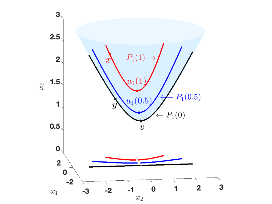
We refer to Figure 1 for an illustration of Pk​(0)P_{k}(0) and some of its translates for the 22-dimensional hyperbolic space.

Refer to caption
(a) (b)
Figure 1: Illustration of the translation (24) on the 22-dimensional hyperbolic space ℍ2\mathbb{H}^{2}. (a) The curve P1​(0)P_{1}(0) and its translates P1​(a)P_{1}(a) for a=0.5a=0.5 and a=1a=1. The points u1​(a)u_{1}(a) are also indicated on the plot. (b) Projections of P1​(a)P_{1}(a) on the x1​x2x_{1}x_{2}-plane for various values of aa.
Lemma 2.10.

Let x∈Pk​(0)x\in P_{k}(0) and a,b∈ℝa,b\in\mathbb{R}, then we have

(x+′uk(a))+′uk(b)=x+′uk(a+b).(x+^{\prime}u_{k}(a))+^{\prime}u_{k}(b)=x+^{\prime}u_{k}(a+b).
Proof.

The proof is provided in Appendix A. ∎

Remark 2.11.

(1) If we put x=vx=v, we have

uk(a)+′uk(b)=uk(a+b),∀a,b∈ℝ.\displaystyle u_{k}(a)+^{\prime}u_{k}(b)=u_{k}(a+b),\qquad\forall~a,b\in\mathbb{R}.

(2) Since uk​(0)=vu_{k}(0)=v, we also have

uk​(a)=−uk​(−a),∀a∈ℝ.u_{k}(a)=-u_{k}(-a),\qquad\forall~a\in\mathbb{R}.

The following lemma is key for the concept of coordinate grid on ℍn\mathbb{H}^{n}. In particular, it shows that the family (24) of translates of Pk​(0)P_{k}(0) covers the entire ℍn\mathbb{H}^{n}; this is similar to how translating a hyperplane xi=0x_{i}=0 along the xix_{i}-axis covers the Euclidean space.

Lemma 2.12.

For any x∈ℍnx\in\mathbb{H}^{n} there exists a unique pair (a,y)∈ℝ×Pk​(0)(a,y)\in\mathbb{R}\times P_{k}(0) such that

x=y+′uk(a).\displaystyle x=y+^{\prime}u_{k}(a). (25)

Furthermore, aa and yy can be expressed as

a=tanh−1(xkx0),y=x−′uk(a).a=\tanh^{-1}\left(\frac{x_{k}}{x_{0}}\right),\qquad y=x-^{\prime}u_{k}(a). (26)
Proof.

The proof is provided in Appendix A. ∎

To illustrate the decomposition (25), we show in Figure 1(a) a point x∈P1​(1)⊂ℍ2x\in P_{1}(1)\subset\mathbb{H}^{2} and its corresponding y∈P1​(0)y\in P_{1}(0) such that x=y+′u1(1)x=y+^{\prime}u_{1}(1). In summary, any point x∈ℍnx\in\mathbb{H}^{n} lies on the hypersurface Pk​(a)P_{k}(a) with aa given by (26), where Pk​(a)P_{k}(a) is the translation of Pk​(0)P_{k}(0) by uk​(a)u_{k}(a). One can think of uk​(a)u_{k}(a) as the kk-th coordinate of xx. Given the uniqueness of the decomposition (25)-(26), we will be using in the sequel the map πk:ℍn→ℝ\pi_{k}:\mathbb{H}^{n}\to\mathbb{R} defined by

πk​(x)=tanh−1⁡(xkx0).\pi_{k}(x)=\tanh^{-1}\left(\frac{x_{k}}{x_{0}}\right). (27)
Corollary 2.13.

Let x∈ℍnx\in\mathbb{H}^{n} with x∈πk−1​(a)x\in\pi_{k}^{-1}(a) for some a∈ℝa\in\mathbb{R}. Then we have

x+′uk(b)∈πk−1(a+b),or equivalently,πk(x+′uk(b))=a+b.x+^{\prime}u_{k}(b)\in\pi_{k}^{-1}(a+b),\qquad\text{or equivalently,}\quad\pi_{k}(x+^{\prime}u_{k}(b))=a+b.
Proof.

From Lemma 2.12, there exists y∈Pk​(0)y\in P_{k}(0) such that

x=y+′uk(a).x=y+^{\prime}u_{k}(a).

Then, by Lemma 2.10, we get

x+′uk(b)=(y+′uk(a))+′uk(b)=y+′uk(a+b).x+^{\prime}u_{k}(b)=(y+^{\prime}u_{k}(a))+^{\prime}u_{k}(b)=y+^{\prime}u_{k}(a+b).

Therefore, x+′uk(b)∈πk−1(a+b)x+^{\prime}u_{k}(b)\in\pi_{k}^{-1}(a+b). ∎

We conclude this section with a simple inequality which will be used later in the paper.

Lemma 2.14.

Let xx and yy be two points in ℍn\mathbb{H}^{n}. Then we have

d(x,y)≥|πk(x)−πk(y)|,∀k=1,2,⋯,n.d(x,y)\geq|\pi_{k}(x)-\pi_{k}(y)|,\qquad\forall~k=1,2,\cdots,n.
Proof.

The proof is provided in Appendix A. ∎

3 Interaction potentials with Newtonian repulsion

In this section, we consider interaction potentials that include Newtonian repulsion, i.e., potentials for which the repulsion component is given by the Green’s function of the negative Laplacian on ℍn\mathbb{H}^{n} [23].

Define

Φ⁡(θ):={−12​π​log⁡(tanh⁡θ2) for ​n=2,1n​α​(n)​∫θ∞1sinhn−1⁡ζ​𝑑ζ for ​n≥3.\displaystyle\Phi(\theta):=\begin{cases}\displaystyle-\frac{1}{2\pi}\log\left(\tanh\frac{\theta}{2}\right)&\text{ for }n=2,\\[10.0pt] \displaystyle\frac{1}{n\alpha(n)}\int^{\infty}_{\theta}\frac{1}{\sinh^{n-1}\zeta}\mathrm{d}\zeta\qquad&\text{ for }n\geq 3.\end{cases} (28)

Note that the case n=2n=2 can in fact be recovered from the expression for general nn, by calculating explicitly the integral. It was shown in [17] that the Green’s function for −Δℍn-\Delta_{\mathbb{H}^{n}} is given by

G⁡(x,y):=Φ⁡(d⁡(x,y)),G(x,y):=\Phi(d(x,y)), (29)

i.e., GG satisfies

Δx​G​(x,y)=−δy.\Delta_{x}G(x,y)=-\delta_{y}. (30)

In this section we consider interaction potentials in the form

K⁡(x,y)=G⁡(x,y)+A⁡(d⁡(x,y)),K(x,y)=G(x,y)+A(d(x,y)), (31)

where GG is given by (29) and A:[0,∞)→ℝA:[0,\infty)\to\mathbb{R}. As discussed in [23], the Green’s function component of KK (referred to in the sequel as Newtonian potential) models repulsive interactions. To balance the repulsion, we take the AA component to model attractive interactions. We refer to Figure 2 for an illustration of several interaction potentials in the form (31); the attraction components are specified later – see (56), (58) and (89).

Figure 2: Interaction potentials in the form (31), with attraction given by (56), (58) and (89), respectively.

Our main goals here are to investigate the qualitative properties of critical points of the interaction energy (1) with KK in the form (31), as well as to study explicit forms of minimizers for certain specific examples of attraction potentials AA. All the equilibria investigated in this section are absolutely continuous probability measures ρ⁡(x)​d​x\rho(x)\mathrm{d}x, with ρ∈L1​(d​x)\rho\in L^{1}(\mathrm{d}x).

Remark 3.1.

Similar to the Euclidean case, the energy (1) corresponding to the Newtonian potential is the square of the H−1H^{-1} norm. Indeed, for ρ∈H−1​(ℍn)\rho\in H^{-1}(\mathbb{H}^{n}) with compact support, by definition of the H−1H^{-1} norm and the divergence theorem, we have:

‖ρ‖H−1​(ℍn)2\displaystyle\left\lVert\rho\right\rVert_{H^{-1}(\mathbb{H}^{n})}^{2} =∫ℍn∥∇u(x)∥ℍn2dx=−∫ℍn(Δℍnu)(x)u(x)dx,\displaystyle=\int_{\mathbb{H}^{n}}\|\nabla u(x)\|_{\mathbb{H}^{n}}^{2}\mathrm{d}x=-\int_{\mathbb{H}^{n}}(\Delta_{\mathbb{H}^{n}}u)(x)u(x)\mathrm{d}x,

where uu satisfies (in the weak sense): −Δℍn​u=ρ\displaystyle{-\Delta_{\mathbb{H}^{n}}u=\rho}. Further, using the fundamental solution, write u⁡(x)=∫ℍnG⁡(x,y)​ρ​(y)​𝑑y\displaystyle{u(x)=\int_{\mathbb{H}^{n}}G(x,y)\rho(y)\mathrm{d}y}, to reach

‖ρ‖H−1​(ℍn)2=∬ℍn×ℍnG⁡(x,y)​ρ​(x)​ρ​(y)​𝑑x​𝑑y.\left\lVert\rho\right\rVert_{H^{-1}(\mathbb{H}^{n})}^{2}=\iint_{\mathbb{H}^{n}\times\mathbb{H}^{n}}G(x,y)\rho(x)\rho(y)\mathrm{d}x\mathrm{d}y. (32)

Regarding the Euler-Lagrange equations, for an interaction potential in the form (31), Λ\Lambda defined in (7) reads:

Λ⁡(x)=∫ℍn(G⁡(x,y)+A⁡(d⁡(x,y))​ρ​(y)​𝑑yCLOSE.\Lambda(x)=\int_{\mathbb{H}^{n}}\left(G(x,y)+A(d(x,y)\right)\rho(y)\mathrm{d}y. (33)

Then, by (30), one finds:

Δ​Λ​(x)={−ρ⁡(x)+∫ℍnΔx​A​(d⁡(x,y))​ρ​(y)​dy for ​x∈supp⁡(ρ),∫ℍnΔx​A​(d⁡(x,y))​ρ​(y)​dy for ​x∉supp⁡(ρ).\Delta\Lambda(x)=\begin{cases}\begin{aligned} &-\rho(x)+\int_{\mathbb{H}^{n}}\Delta_{x}A(d(x,y))\rho(y)\mathrm{d}y\qquad\text{ for }x\in\mathrm{supp}(\rho),\\ &\int_{\mathbb{H}^{n}}\Delta_{x}A(d(x,y))\rho(y)\mathrm{d}y\hskip 66.86414pt\text{ for }x\notin\mathrm{supp}(\rho).\end{aligned}\end{cases} (34)

For critical points of the energy (or equivalently, equilibrium solutions of model (2)), Λ⁡(x)\Lambda(x) is identically equal to a constant in the support of ρ\rho (see (6a)). Hence, Δ​Λ=0\Delta\Lambda=0 in supp⁡(ρ)\mathrm{supp}(\rho), and the first equation in (34) leads to the following integral equation for equilibrium densities ρ\rho:

ρ⁡(x)=∫supp⁡(ρ)Δx​A​(d⁡(x,y))​ρ​(y)​𝑑y, for ​x∈supp⁡(ρ).\rho(x)=\int_{\mathrm{supp}(\rho)}\Delta_{x}A(d(x,y))\rho(y)\mathrm{d}y,\qquad\text{ for }x\in\mathrm{supp}(\rho). (35)

3.1 Equilibria supported on geodesic balls

We consider equilibria of the aggregation model (2) that are supported on geodesic balls centred at the vertex vv, and study their qualitative properties. To prove the main result (Theorem 3.3) on the radial symmetry and the monotonicity of such states, we employ the method of moving planes by adapting it to the hyperbolic space.

Before we present the main result, we introduce the reflection on the hyperbolic space ℍn\mathbb{H}^{n}. In the Euclidean space ℝn\mathbb{R}^{n}, the reflection by a hyperplane x1=ax_{1}=a is given by the map:

(x1,x2,⋯,xn)↦(2​a−x1,x2,⋯,xn).\displaystyle(x_{1},x_{2},\cdots,x_{n})\mapsto(2a-x_{1},x_{2},\cdots,x_{n}). (36)

The reflection map (36) can be divided into three maps as follows:

(x1,x2,⋯,xn)↦(x1−a,x2,⋯,xn)↦(a−x1,x2,⋯,xn)↦(2​a−x1,x2,⋯,xn).\displaystyle(x_{1},x_{2},\cdots,x_{n})\mapsto(x_{1}-a,x_{2},\cdots,x_{n})\mapsto(a-x_{1},x_{2},\cdots,x_{n})\mapsto(2a-x_{1},x_{2},\cdots,x_{n}). (37)

The first map is the translation in the x1x_{1} coordinate by −a-a, the second map is the reflection by the hyperplane x1=0x_{1}=0, and the third map is the translation in the x1x_{1} coordinate by aa.

We apply now a similar argument to define the reflection on ℍn\mathbb{H}^{n}. We present the reflection corresponding to coordinate x1x_{1}, the reflections corresponding to coordinates x2,…,xnx_{2},\dots,x_{n} are similar. First, we define the reference hypersurface for the reflection. For the Euclidean space, this is a regular flat hyperplane, however, for the hyperbolic space we choose the hypersurface to be P1​(a)P_{1}(a) defined in (24) (see also Figure 1). For the translation on ℍn\mathbb{H}^{n} we use the +′+^{\prime} operation (see Definition 2.1), and take the translation by ±a\pm a in the x1x_{1} coordinate, to be x↦x±′u1(a)x\mapsto x\pm^{\prime}u_{1}(a) (see (24)). Finally, analogous to the reflection by the hyperplane x1=0x_{1}=0 in the Euclidean space, on ℍn\mathbb{H}^{n} we have reflection by the hypersurface P1​(0)={x∈ℍn:x1=0}P_{1}(0)=\{x\in\mathbb{H}^{n}:x_{1}=0\}, which we define it to be:

R1:(x0,x1,x2,⋯,xn)∈ℍn∣⟶(x0,−x1,x2,⋯,xn)∈ℍn.R_{1}:(x_{0},x_{1},x_{2},\cdots,x_{n})\in\mathbb{H}^{n}\shortmid\!\longrightarrow(x_{0},-x_{1},x_{2},\cdots,x_{n})\in\mathbb{H}^{n}.

Following the map sequence in (37) (translation by −a-a, reflection, translation by aa), we express the reflection across an arbitrary hypersurface P1​(a)P_{1}(a) on ℍn\mathbb{H}^{n} as:

x∣⟶x−′u1(a)∣⟶R1(x−′u1(a))∣⟶R1(x−′u1(a))+′u1(a).x\shortmid\!\longrightarrow x-^{\prime}u_{1}(a)\shortmid\!\longrightarrow R_{1}(x-^{\prime}u_{1}(a))\shortmid\!\longrightarrow R_{1}(x-^{\prime}u_{1}(a))+^{\prime}u_{1}(a). (38)

This sequence of three maps is illustrated schematically in Figure 3. Written compactly, the reflection map above reads:

x∣⟶xa:=R1(x−′u1(a))+′u1(a).x\shortmid\!\longrightarrow x^{a}:=R_{1}(x-^{\prime}u_{1}(a))+^{\prime}u_{1}(a). (39)

For a better understanding of the reflection map, let us express the reflected point xax^{a} in coordinates. From the definition of −′-^{\prime} and u1​(a)u_{1}(a) (see (20) and (23)), we have

{(x−′u1(a))0=x0cosha−x1sinha,(x−′u1(a))1=x1cosha−x0sinha,(x−′u1(a))j=xj,∀2≤j≤n.\begin{cases}(x-^{\prime}u_{1}(a))_{0}=x_{0}\cosh a-x_{1}\sinh a,\\ (x-^{\prime}u_{1}(a))_{1}=x_{1}\cosh a-x_{0}\sinh a,\\ (x-^{\prime}u_{1}(a))_{j}=x_{j},\qquad\forall~2\leq j\leq n.\end{cases}

Then, by the definition of the reflection R1R_{1}, we have

{(R1(x−′u1(a)))0=x0cosha−x1sinha,(R1(x−′u1(a)))1=−x1cosha+x0sinha,(R1(x−′u1(a)))j=xj,∀2≤j≤n.\begin{cases}(R_{1}(x-^{\prime}u_{1}(a)))_{0}=x_{0}\cosh a-x_{1}\sinh a,\\ (R_{1}(x-^{\prime}u_{1}(a)))_{1}=-x_{1}\cosh a+x_{0}\sinh a,\\ (R_{1}(x-^{\prime}u_{1}(a)))_{j}=x_{j},\quad\forall~2\leq j\leq n.\end{cases}

Finally, we use the definition of +′+^{\prime} and u1​(a)u_{1}(a) to get

{(R1(x−′u1(a))+′u1(a))0=(x0​cosh⁡a−x1​sinh⁡a)​cosh⁡a+(−x1​cosh⁡a+x0​sinh⁡a)​sinh⁡a=x0​cosh⁡2​a−x1​sinh⁡2​a,(R1(x−′u1(a))+′u1(a))1=(−x1​cosh⁡a+x0​sinh⁡a)​cosh⁡a−(x0​cosh⁡a−x1​sinh⁡a)​sinh⁡a=−x1​cosh⁡2​a+x0​sinh⁡2​a,(R1(x−′u1(a))+′u1(a))j=xj,∀2≤j≤n.\begin{cases}(R_{1}(x-^{\prime}u_{1}(a))+^{\prime}u_{1}(a))_{0}&=(x_{0}\cosh a-x_{1}\sinh a)\cosh a+(-x_{1}\cosh a+x_{0}\sinh a)\sinh a\\ &=x_{0}\cosh 2a-x_{1}\sinh 2a,\\[2.0pt] (R_{1}(x-^{\prime}u_{1}(a))+^{\prime}u_{1}(a))_{1}&=(-x_{1}\cosh a+x_{0}\sinh a)\cosh a-(x_{0}\cosh a-x_{1}\sinh a)\sinh a\\ &=-x_{1}\cosh 2a+x_{0}\sinh 2a,\\[2.0pt] (R_{1}(x-^{\prime}u_{1}(a))+^{\prime}u_{1}(a))_{j}&=x_{j},\quad\forall~2\leq j\leq n.\end{cases}

Therefore, we can express the reflection (39) in coordinates, by:

x=(x0,x1,⋯,xn)∣⟶xa=(x0​cosh⁡2​a−x1​sinh⁡2​a,−x1​cosh⁡2​a+x0​sinh⁡2​a,x2,⋯,xn).x=(x_{0},x_{1},\cdots,x_{n})\shortmid\!\longrightarrow x^{a}=(x_{0}\cosh 2a-x_{1}\sinh 2a,-x_{1}\cosh 2a+x_{0}\sinh 2a,x_{2},\cdots,x_{n}).
x1x_{1}x2x_{2}P1​(a)P_{1}(a)AABBCCDDx↦x−′u1(a)x\mapsto x-^{\prime}u_{1}(a)(x0,x1,x2)↦(x0,−x1,x2)(x_{0},x_{1},x_{2})\mapsto(x_{0},-x_{1},x_{2})x↦x+′u1(a)x\mapsto x+^{\prime}u_{1}(a)
Figure 3: Schematic illustration (in the x1​x2x_{1}x_{2}-plane) of the reflection on ℍ2\mathbb{H}^{2} across the hypersurface P1​(a)P_{1}(a) – see (39). Point AA reflects into point DD, as the result of three maps A↦BA\mapsto B (translation by −u1​(a)-u_{1}(a)), B↦CB\mapsto C (reflection across P1​(0)=x0​x2−P_{1}(0)=x_{0}x_{2}-plane), and C↦DC\mapsto D (translation by u1​(a)u_{1}(a).
Remark 3.2.

The following properties can be checked easily:

  1. 1.

    x=(xa)ax=(x^{a})^{a}, for all x∈ℍnx\in\mathbb{H}^{n}.

  2. 2.

    The set of fixed points for the reflection (39) is P1​(a)P_{1}(a).

  3. 3.

    The reflection map (39) is an isometry on ℍn\mathbb{H}^{n}.

We present now the main result of this subsection.

Theorem 3.3.

Consider the aggregation model (2) with an interaction potential in the form (31). Let ρ\rho be a bounded equilibrium solution of model (2) that is supported in the geodesic ball BR​(v)B_{R}(v), for some R>0R>0. Let F⁡(d⁡(x,y)):=Δx​A​(d⁡(x,y))F(d(x,y)):=\Delta_{x}A(d(x,y)) and assume F⁡(d⁡(x,⋅))F(d(x,\cdot)) is locally integrable for all xx. Then, provided FF is a monotone function, ρ\rho is radially symmetric and monotone about the vertex vv. Specifically, (i) if FF is decreasing, then ρ\rho is radially symmetric and monotonically decreasing about the vertex vv, and (ii) if FF is increasing, then ρ\rho is radially symmetric and monotonically increasing about vv.

Proof.

Since ρ\rho is an equilibrium solution, we use (35) to write:

ρ⁡(x)={∫BR​(v)F⁡(d⁡(x,y))​ρ​(y)​𝑑y for ​x∈BR​(v),0otherwise.\rho(x)=\begin{cases}\displaystyle\int_{B_{R}(v)}F(d(x,y))\rho(y)\mathrm{d}y\qquad&\text{ for }x\in B_{R}(v),\\[10.0pt] 0&\text{otherwise}.\end{cases} (40)

We define the reflection ρa\rho_{a} of ρ\rho across the plane P1​(a)P_{1}(a) by:

ρa​(x)=ρ⁡(xa).\rho_{a}(x)=\rho(x^{a}).

From (40) we have

ρa​(x)={∫BR​(v)F⁡(d⁡(xa,y))​ρ​(y)​𝑑yx∈BR​(va),0otherwise.\rho_{a}(x)=\begin{cases}\displaystyle\int_{B_{R}(v)}F(d(x^{a},y))\rho(y)\mathrm{d}y\qquad&x\in B_{R}(v^{a}),\\[10.0pt] 0&\text{otherwise}.\end{cases}

Also, we set

Σa={x∈BR​(v):π1​(x)≥a}.\Sigma_{a}=\{x\in B_{R}(v):\pi_{1}(x)\geq a\}.

We apply the method of moving planes and compare ρ⁡(x)\rho(x) and ρa​(x)\rho_{a}(x) on Σa\Sigma_{a}. If x∉BR​(va)x\not\in B_{R}(v^{a}), then we know that ρa​(x)=0\rho_{a}(x)=0. Since ρ⁡(x)≥0\rho(x)\geq 0, we can conclude that ρ⁡(x)−ρa​(x)≥0\rho(x)-\rho_{a}(x)\geq 0 for all x∈Σa∖BR​(va)x\in\Sigma_{a}\setminus B_{R}(v^{a}).

Consider the case x∈Σa∩BR​(va)x\in\Sigma_{a}\cap B_{R}(v^{a}). By (40) we write ρ⁡(x)\rho(x) as

ρ⁡(x)=∫BR​(v)∩ΣaF⁡(d⁡(x,y))​ρ​(y)​𝑑y+∫BR​(v)∖ΣaF⁡(d⁡(x,y))​ρ​(y)​𝑑y.\rho(x)=\int_{B_{R}(v)\cap\Sigma_{a}}F(d(x,y))\rho(y)\mathrm{d}y+\int_{B_{R}(v)\setminus\Sigma_{a}}F(d(x,y))\rho(y)\mathrm{d}y. (41)

We use that the reflection map (39) is an isometry to rewrite the second integral above in reflected form (reflect the domain of integration, as well as xx and yy). The image of BR​(v)∖ΣaB_{R}(v)\setminus\Sigma_{a} under the reflection map (39) is BR​(va)∩ΣaB_{R}(v^{a})\cap\Sigma_{a}. Also use ρ⁡(y)=ρa​(ya)\rho(y)=\rho_{a}(y^{a}) to get from (41):

ρ⁡(x)\displaystyle\rho(x) =∫BR​(v)∩ΣaF⁡(d⁡(x,y))​ρ​(y)​𝑑y+∫BR​(va)∩ΣaF⁡(d⁡(xa,ya))​ρa​(ya)​d​ya\displaystyle=\int_{B_{R}(v)\cap\Sigma_{a}}F(d(x,y))\rho(y)\mathrm{d}y+\int_{B_{R}(v^{a})\cap\Sigma_{a}}F(d(x^{a},y^{a}))\rho_{a}(y^{a})\mathrm{d}y^{a}
=∫BR​(v)∩ΣaF⁡(d⁡(x,y))​ρ​(y)​𝑑y+∫BR​(va)∩ΣaF⁡(d⁡(xa,y))​ρa​(y)​𝑑y,\displaystyle=\int_{B_{R}(v)\cap\Sigma_{a}}F(d(x,y))\rho(y)\mathrm{d}y+\int_{B_{R}(v^{a})\cap\Sigma_{a}}F(d(x^{a},y))\rho_{a}(y)\mathrm{d}y,

where for the second equal sign we simply renamed the variable yay^{a} to yy.

Since ρ\rho and ρa\rho_{a} are zero outside BR​(v)B_{R}(v) and BR​(va)B_{R}(v^{a}), respectively, we can also write the expression above as:

ρ⁡(x)=∫ΣaF⁡(d⁡(x,y))​ρ​(y)​𝑑y+∫ΣaF⁡(d⁡(xa,y))​ρa​(y)​𝑑y.\rho(x)=\int_{\Sigma_{a}}F(d(x,y))\rho(y)\mathrm{d}y+\int_{\Sigma_{a}}F(d(x^{a},y))\rho_{a}(y)\mathrm{d}y. (42)

By replacing xx with xax^{a} in (42), we can obtain the following expression for ρa\rho_{a}:

ρa​(x)=∫ΣaF⁡(d⁡(xa,y))​ρ​(y)​𝑑y+∫ΣaF⁡(d⁡(x,y))​ρa​(y)​𝑑y.\rho_{a}(x)=\int_{\Sigma_{a}}F(d(x^{a},y))\rho(y)dy+\int_{\Sigma_{a}}F(d(x,y))\rho_{a}(y)\mathrm{d}y. (43)

From (42) and (43) we calculate the difference ρ​(x)−ρa​(x)\rho(x)-\rho_{a}(x) for x∈Σa∩BR​(va)x\in\Sigma_{a}\cap B_{R}(v^{a}) as:

ρ⁡(x)−ρa​(x)=∫Σa(F⁡(d⁡(x,y))−F⁡(d⁡(xa,y)))​(ρ⁡(y)−ρa​(y))​𝑑y.\rho(x)-\rho_{a}(x)=\int_{\Sigma_{a}}(F(d(x,y))-F(d(x^{a},y)))(\rho(y)-\rho_{a}(y))\mathrm{d}y. (44)

We can show that

d⁡(x,y)≤d⁡(xa,y), for all ​x,y∈Σa.d(x,y)\leq d(x^{a},y),\qquad\text{ for all }x,y\in\Sigma_{a}. (45)

Indeed, without loss of generality, it is enough to proof the case a=0a=0. Let x=(x0,x1,⋯,xn)x=(x_{0},x_{1},\cdots,x_{n}) and y=(y0,y1,⋯,yn)y=(y_{0},y_{1},\cdots,y_{n}). Since x,y∈Σ0x,y\in\Sigma_{0}, we have x1,y1≥0x_{1},y_{1}\geq 0. This yields that

cosh⁡(d⁡(x,y))=x0​y0−x1​y1−⋯−xn​yn≤x0​y0+x1​y1−⋯−xn​yn=cosh⁡(d⁡(x0,y)),\cosh\left(d(x,y)\right)=x_{0}y_{0}-x_{1}y_{1}-\cdots-x_{n}y_{n}\leq x_{0}y_{0}+x_{1}y_{1}-\cdots-x_{n}y_{n}=\cosh\left(d(x^{0},y)\right),

which implies the desired result.

Consider now the following two cases.

Case (i): FF is decreasing. Since FF is decreasing and (45) holds, we have

F⁡(d⁡(x,y))−F⁡(d⁡(xa,y))≥0, for all ​x∈Σa∩BR​(va)​ and ​y∈Σa.F(d(x,y))-F(d(x^{a},y))\geq 0,\qquad\text{ for all }x\in\Sigma_{a}\cap B_{R}(v^{a})\text{ and }y\in\Sigma_{a}. (46)

We will show that

ρa≤ρ, on ​Σa,\rho_{a}\leq\rho,\qquad\text{ on }\Sigma_{a},

for all a∈(−R,0)a\in(-R,0), which implies that ρ\rho is monotonically decreasing about the vertex, in the x1x_{1} direction.

Assume first that there exists a0∈(−R,0)a_{0}\in(-R,0) such that

ρa0​(x)≤ρ⁡(x), for all ​x∈Σa0,\rho_{a_{0}}(x)\leq\rho(x),\qquad\text{ for all }x\in\Sigma_{a_{0}}, (47)

and show that a0a_{0} can be extended to the origin. Indeed, suppose by contradiction that (47) holds, but a0a_{0} cannot be extended, and take a∈(a0,a0+ϵ)a\in(a_{0},a_{0}+\epsilon), with ϵ>0\epsilon>0. Define

Σa−={x∈Σa:ρ⁡(x)<ρa​(x)}.\Sigma_{a}^{-}=\{x\in\Sigma_{a}:\rho(x)<\rho_{a}(x)\}.

Then, from (44) and (46), for any x∈Σa−x\in\Sigma_{a}^{-}, we have:

0<ρa​(x)−ρ⁡(x)≤∫Σa−(F⁡(d⁡(x,y))−F⁡(d⁡(xa,y)))​(ρa​(y)−ρ⁡(y))​𝑑y.0<\rho_{a}(x)-\rho(x)\leq\int_{\Sigma_{a}^{-}}(F(d(x,y))-F(d(x^{a},y)))(\rho_{a}(y)-\rho(y))\mathrm{d}y.

Therefore,

‖ρa−ρ‖L∞​(Σa−)≤‖ρa−ρ‖L∞​(Σa−)​supx∈Σa−∫Σa−(F⁡(d⁡(x,y))−F⁡(d⁡(xa,y)))​𝑑y.\|\rho_{a}-\rho\|_{L^{\infty}(\Sigma_{a}^{-})}\leq\|\rho_{a}-\rho\|_{L^{\infty}(\Sigma_{a}^{-})}\sup_{x\in\Sigma_{a}^{-}}\int_{\Sigma_{a}^{-}}(F(d(x,y))-F(d(x^{a},y)))\mathrm{d}y. (48)

The function under the integral on the right-hand-side is locally integrable. Also, by (44), it holds that ρ​(x)>ρa0​(x)\rho(x)>\rho_{a_{0}}(x) in the interior of Σa0\Sigma_{a_{0}}, implying that the closure of Σa0−\Sigma_{a_{0}}^{-} has measure 00. As lima→a0Σa−⊂Σa0−¯\lim_{a\to a_{0}}\Sigma_{a}^{-}\subset\overline{\Sigma_{a_{0}}^{-}}, we infer that the measure of Σa−\Sigma_{a}^{-} approaches 00 as a→a0a\to a_{0}. Therefore, we can choose ϵ\epsilon small enough such that

supx∈Σa−∫Σa−(F⁡(d⁡(x,y))−F⁡(d⁡(xa,y)))​𝑑y≤12.\sup_{x\in\Sigma_{a}^{-}}\int_{\Sigma_{a}^{-}}(F(d(x,y))-F(d(x^{a},y)))\mathrm{d}y\leq\frac{1}{2}.

From (48) we then infer that ‖ρa−ρ‖L∞​(Σa−)\|\rho_{a}-\rho\|_{{L^{\infty}}(\Sigma_{a}^{-})} =  0, which implies that Σa−\Sigma_{a}^{-} is empty. Consequently, a0a_{0} is not maximal and we reached a contradiction.

To show that there exists a0∈(−R,0)a_{0}\in(-R,0) with the property (47), note that (47) holds for a0=−Ra_{0}=-R. Then, by an argument entirely similar to the one made in the previous step, one can infer that the plane a0=−Ra_{0}=-R can be moved further to the right, while (47) still holds.

A similar argument can be made using hypersufaces with a>0a>0. Finally, since the direction x1x_{1} can be chosen arbitrarily, we conclude that ρ\rho is radially symmetric and decreasing about the vertex vv. This concludes the proof for case (i).

Case (ii): FF is increasing. From a similar argument as for case (i), one can show that ρ\rho is radially symmetric and increasing about the vertex vv. ∎

We now turn the attention on radially symmetric equilibria that are local minimizers of the energy (see Lemma 2.1).

Proposition 3.4.

Let KK be an interaction potential in the form (31), and let ρ\rho be a bounded, radially symmetric equilibrium solution of model (2) that is supported in the geodesic ball BR​(v)B_{R}(v), for some R>0R>0. Assume that A:[0,∞)→ℝA:[0,\infty)\to\mathbb{R} satisfies Δx​A​(d⁡(x,y))≥0\Delta_{x}A(d(x,y))\geq 0 for all x,y∈ℍnx,y\in\mathbb{H}^{n}. Then ρ\rho satisfies the necessary condition (6) for being a local energy minimizer.

Proof.

Since ρ\rho is an equilibrium solution, it satisfies the first equation of (6). It remains to show (6b). By using (34), we write:

Δ​Λ​(x)={0if ​x∈BR​(v),∫ℍnΔxA(d(x,y))ρ(y)dy,if ​x∉BR​(v).\displaystyle\Delta\Lambda(x)=\begin{cases}0\qquad&\text{if }x\in B_{R}(v),\\[3.0pt] \displaystyle\int_{\mathbb{H}^{n}}\Delta_{x}A(d(x,y))\rho(y)\mathrm{d}y,\qquad&\text{if }x\not\in B_{R}(v).\end{cases} (49)

As KK and ρ\rho are radially symmetric, Λ\Lambda has radial symmetry as well. Hence, we can define Λ~:[0,∞)→R\tilde{\Lambda}:[0,\infty)\to R by:

Λ~​(r):=Λ​(x),\tilde{\Lambda}(r):=\Lambda(x), (50)

for some x∈∂Br​(v)x\in\partial B_{r}(v). In particular, by (6a), Λ~​(r)=λ\tilde{\Lambda}(r)=\lambda for 0≤r≤R0\leq r\leq R.

For r>Rr>R, use the divergence theorem in Br​(v)B_{r}(v) to obtain that

∫Br​(v)Δ​Λ​(x)​𝑑x=∫∂Br​(v)∇Λ​(x)⋅𝑑n→=|∂Br​(v)|​Λ~′​(r).\int_{B_{r}(v)}\Delta\Lambda(x)dx=\int_{\partial B_{r}(v)}\nabla\Lambda(x)\cdot\mathrm{d}\vec{n}=|\partial B_{r}(v)|\tilde{\Lambda}^{\prime}(r). (51)

From Δx​A​(d⁡(x,y))≥0\Delta_{x}A(d(x,y))\geq 0 and (49), it follows that Δ​Λ​(x)≥0\Delta\Lambda(x)\geq 0 for all xx. Consequently, using the equation above, we infer that Λ~\tilde{\Lambda} is a non-decreasing function, and conclude that

{Λ~​(r)=λif ​0≤r≤R,Λ~​(r)≥λif ​r>R.\begin{cases}\tilde{\Lambda}(r)=\lambda\qquad\text{if }0\leq r\leq R,\\[3.0pt] \tilde{\Lambda}(r)\geq\lambda\qquad\text{if }r>R.\end{cases}

This shows that the necessary condition (6b) for a local minimizer is also satisfied. ∎

The following proposition shows that for potentials with Δ​A>0\Delta A>0, radially symmetric local minimizers must have a geodesic ball as their support.

Proposition 3.5.

Let KK be an interaction potential in the form (31), where A:[0,∞)→ℝA:[0,\infty)\to\mathbb{R} satisfies Δx​A​(d⁡(x,y))>0\Delta_{x}A(d(x,y))>0 for all x,y∈ℍnx,y\in\mathbb{H}^{n}. If ρ\rho is a bounded, radially symmetric local minimizer of the interaction energy, then there exists R>0R>0 such that supp​(ρ)=BR​(v)\mathrm{supp}(\rho)=B_{R}(v).

Proof.

As ρ\rho is bounded and radially symmetric, its support can be expressed as

supp⁡(ρ)=⋃r∈C∂Br​(v),\mathrm{supp}(\rho)=\bigcup_{r\in C}\partial B_{r}(v),

where C⊂[0,∞)C\subset[0,\infty) is a compact set.

First note that Λ\Lambda is radially symmetric (see (50)) and Λ~​(r)=λ\tilde{\Lambda}(r)=\lambda for r∈Cr\in C. Also, from

Δ​Λ​(x)={0if ​x∈supp⁡(ρ),∫ℍnΔx​A​(d⁡(x,y))​ρ​(y)​𝑑y>0if ​x∉supp⁡(ρ),\Delta\Lambda(x)=\begin{cases}0\qquad&\text{if }x\in\mathrm{supp}(\rho),\\[3.0pt] \displaystyle\int_{\mathbb{H}^{n}}\Delta_{x}A(d(x,y))\rho(y)\mathrm{d}y>0\qquad&\text{if }x\not\in\mathrm{supp}(\rho),\end{cases}

and (51), we find that:

Λ~′​(r)>0if ​r∉C.\displaystyle\tilde{\Lambda}^{\prime}(r)>0\qquad\text{if }r\not\in C. (52)

Since CC is a compact set in [0,∞)[0,\infty), we can express CC as a union of disjoint closed intervals as follows:

C=[a1,b1]∪[a2,b2]∪⋯∪[ak,bk],C=[a_{1},b_{1}]\cup[a_{2},b_{2}]\cup\cdots\cup[a_{k},b_{k}],

where 0≤a1<b1<a2<b2<⋯<ak<bk0\leq a_{1}<b_{1}<a_{2}<b_{2}<\cdots<a_{k}<b_{k}. If k≥2k\geq 2, then

Λ~​(b1)=Λ~​(a2)(=λ).\tilde{\Lambda}(b_{1})=\tilde{\Lambda}(a_{2})\;(=\lambda).

However, this contradicts (52), so we conclude that k=1k=1. Now assume that 0<a10<a_{1}. From (52), we have

Λ~​(0)<Λ~​(a1),\tilde{\Lambda}(0)<\tilde{\Lambda}(a_{1}),

but this cannot occur for a local minimizer (see (6b)).

We conclude that a1=0a_{1}=0, and C=[0,b1]C=[0,b_{1}]. By setting R=b1R=b_{1}, we then have

supp⁡(ρ)=⋃r∈[0,R]∂Br​(v)=BR​(v).\mathrm{supp}(\rho)=\bigcup_{r\in[0,R]}\partial B_{r}(v)=B_{R}(v).

∎

3.2 Explicit forms of radially symmetric equilibria

We first find some explicit expressions of equilibria for certain interaction potentials in the form (31). These equilibria are radially symmetric and with supp​(ρ)=DR​(v)\mathrm{supp}(\rho)=D_{R}(v), R>0R>0.

Denote

ρ~​(d​(v,x)):=ρ​(x).\tilde{\rho}(d(v,x)):=\rho(x). (53)

Then, the integral equation (35) reads:

ρ~​(θx)=∫0R∫𝕊n(A′′​(θx​y)+(n−1)​coth⁡(θx​y)​A′​(θx​y))​ρ~​(θy)​sinhn−1⁡θy​d​σy​d​θy,\tilde{\rho}(\theta_{x})=\int_{0}^{R}\int_{\mathbb{S}^{n}}\left(A^{\prime\prime}(\theta_{xy})+(n-1)\coth(\theta_{xy})A^{\prime}(\theta_{xy})\right)\tilde{\rho}(\theta_{y})\sinh^{n-1}\theta_{y}\,\mathrm{d}\sigma_{y}\mathrm{d}\theta_{y}, (54)

that holds for all x∈DR​(v)x\in D_{R}(v), where θx:=d⁡(v,x)\theta_{x}:=d(v,x) and θx​y:=d⁡(x,y)\theta_{xy}:=d(x,y). Note that we used (12) to write:

Δx​A​(d⁡(x,y))=A′′​(d⁡(x,y))+(n−1)​coth⁡(d⁡(x,y))​A′​(d⁡(x,y)).\displaystyle\Delta_{x}A(d(x,y))=A^{\prime\prime}(d(x,y))+(n-1)\coth(d(x,y))A^{\prime}(d(x,y)). (55)

The two main specific examples of attractive potentials investigated here are:

(i) Constant Laplacian attraction:

Ac​(θ)=∫0θ∫0θ∗sinhn−1⁡ξ​𝑑ξsinhn−1⁡θ∗​d​θ∗.\displaystyle A_{c}(\theta)=\int_{0}^{\theta}\frac{\int_{0}^{\theta_{*}}\sinh^{n-1}\xi\mathrm{d}\xi}{\sinh^{n-1}\theta_{*}}\,\mathrm{d}\theta_{*}. (56)

This is a very important example for applications; AcA_{c} has the property that

Δx​Ac​(d⁡(x,y))=1,\Delta_{x}A_{c}(d(x,y))=1, (57)

and leads to equilibria that are constant within their support.

(ii) Hyperbolic-cosine attraction:

Ah​(θ)=cosh⁡θ−1n.\displaystyle A_{h}(\theta)=\frac{\cosh\theta-1}{n}. (58)

This potential satisfies (use (55)):

Δx​Ah​(d⁡(x,y))=cosh⁡(d⁡(x,y)).\Delta_{x}A_{h}(d(x,y))=\cosh(d(x,y)).

We will show that the energy functional in this case is strictly convex, and we will find explicitly the global minimizer.

Constant Laplacian attraction.

Consider the interaction potential (31) with attraction given by (56). Since AcA_{c} satisfies (57), it is immediate to check that the following density distribution is a solution of (54):

ρc​(x)={1 if ​d​(v,x)≤Rc,0 if ​d​(v,x)>Rc,\displaystyle\rho_{c}(x)=\begin{cases}1\qquad\text{ if }d(v,x)\leq R_{c},\\[2.0pt] 0\qquad\text{ if }d(v,x)>R_{c},\end{cases} (59)

where RcR_{c} satisfies

Vol⁡(DRc​(v))=n​α​(n)​∫0Rcsinhn−1⁡θ​𝑑θ=1.\displaystyle\mathrm{Vol}(D_{R_{c}}(v))=n\alpha(n)\int_{0}^{R_{c}}\sinh^{n-1}\theta\mathrm{d}\theta=1. (60)

Hence, ρc\rho_{c} is an equilibrium solution, and by Proposition 3.4, it satisfies the necessary conditions for a local minimizer. This configuration was studied in [23] as an attractor for the aggregation equation (2).

Hyperbolic-cosine attraction.

We consider now the interaction potential (31) with attraction given by (58). We will show that the following density distribution is a global minimizer of the interaction energy:

ρh​(x)={cosh⁡(d⁡(v,x))α⁡(n)​sinhn⁡Rh if ​d​(v,x)≤Rh,0 if ​d​(v,x)>Rh,\displaystyle\rho_{h}(x)=\begin{cases}\displaystyle\frac{\cosh(d(v,x))}{\alpha(n)\sinh^{n}R_{h}}&\qquad\text{ if }d(v,x)\leq R_{h},\\[10.0pt] 0&\qquad\text{ if }d(v,x)>R_{h},\end{cases} (61)

where Rh>0R_{h}>0 satisfies

n​α​(n)​∫0Rhsinhn−1⁡θ​cosh2⁡θ​𝑑θ=1.\displaystyle n\alpha(n)\int_{0}^{R_{h}}\sinh^{n-1}\theta\cosh^{2}\theta\,\mathrm{d}\theta=1. (62)

We will show that (61) is a solution of (54). By rotational symmetry, use notation:

ρ~h​(d⁡(v,x)):=ρh​(x).\tilde{\rho}_{h}(d(v,x)):=\rho_{h}(x).

The hyperbolic law of cosines on ℍn\mathbb{H}^{n} states:

cosh⁡(d⁡(x,y))=cosh⁡(d⁡(x,v))​cosh⁡(d⁡(y,v))−sinh⁡(d⁡(x,v))​sinh⁡(d⁡(y,v))​cos⁡∠⁡(x​v​y).\displaystyle\cosh(d(x,y))=\cosh(d(x,v))\cosh(d(y,v))-\sinh(d(x,v))\sinh(d(y,v))\cos\angle(xvy). (63)

From (63) we compute, using polar coordinates for yy and the rotational symmetry of ρh\rho_{h}:

∫ℍncosh⁡(d⁡(x,y))​ρh​(y)​𝑑y\displaystyle\int_{\mathbb{H}^{n}}\cosh(d(x,y))\rho_{h}(y)\mathrm{d}y
=∫0Rh∫𝕊n−1(cosh⁡(d⁡(x,v))​cosh⁡θ−sinh⁡(d⁡(x,v))​sinh⁡θ​cos⁡∠⁡(x​v​y))​ρ~h​(θ)​sinhn−1⁡θ​d​σy​𝑑θ,\displaystyle\quad=\int_{0}^{R_{h}}\int_{\mathbb{S}^{n-1}}\left(\cosh(d(x,v))\cosh\theta-\sinh(d(x,v))\sinh\theta\cos\angle(xvy)\right)\tilde{\rho}_{h}(\theta)\sinh^{n-1}\theta\,\mathrm{d}\sigma_{y}\mathrm{d}\theta,

where we also used that supp⁡(ρh)=DRh​(v)\mathrm{supp}(\rho_{h})=D_{R_{h}}(v). Then, using

∫𝕊n−1cos⁡∠⁡(x​v​y)​d​σy\displaystyle\int_{\mathbb{S}^{n-1}}\cos\angle(xvy)\mathrm{d}\sigma_{y} =12​∫𝕊n(cos⁡∠⁡(x​v​y)+cos⁡∠⁡(x​v​(−y))​d​σyCLOSE\displaystyle=\frac{1}{2}\int_{\mathbb{S}^{n}}(\cos\angle(xvy)+\cos\angle(xv(-y))\mathrm{d}\sigma_{y}
=12​∫𝕊n(cos⁡∠⁡(x​v​y)+cos⁡(π+∠⁡(x​v​y))​d​σyCLOSE\displaystyle=\frac{1}{2}\int_{\mathbb{S}^{n}}(\cos\angle(xvy)+\cos(\pi+\angle(xvy))\mathrm{d}\sigma_{y}
=0,\displaystyle=0,

in the equation above, we have

∫ℍncosh⁡(d⁡(x,y))​ρh​(y)​𝑑y=n​α​(n)​cosh⁡(d⁡(v,x))​∫0Rhcosh⁡θ​ρ~h​(θ)​sinhn−1⁡θ​𝑑θ.\int_{\mathbb{H}^{n}}\cosh(d(x,y))\rho_{h}(y)\mathrm{d}y=n\alpha(n)\cosh(d(v,x))\int_{0}^{R_{h}}\cosh\theta\tilde{\rho}_{h}(\theta)\sinh^{n-1}\theta\,\mathrm{d}\theta. (64)

Consequently, to show that ρh\rho_{h} is a solution of (54), we need to show:

ρ~h​(d⁡(v,x))=n​α​(n)​cosh⁡(d⁡(v,x))​∫0Rhcosh⁡θ​ρ~h​(θ)​sinhn−1⁡θ​𝑑θ.\tilde{\rho}_{h}(d(v,x))=n\alpha(n)\cosh(d(v,x))\int_{0}^{R_{h}}\cosh\theta\tilde{\rho}_{h}(\theta)\sinh^{n-1}\theta\,\mathrm{d}\theta.

Indeed, by substituting (61) into the right-hand-side above, one computes:

n​α​(n)​cosh⁡(d⁡(v,x))​∫0Rhcosh2⁡θ​sinhn−1⁡θα⁡(n)​sinhn⁡Rh​𝑑θ\displaystyle n\alpha(n)\cosh(d(v,x))\int_{0}^{R_{h}}\frac{\cosh^{2}\theta\sinh^{n-1}\theta}{\alpha(n)\sinh^{n}R_{h}}d\theta
=cosh⁡(d⁡(v,x))α⁡(n)​sinhn⁡Rh​n​α​(n)​∫0Rhcosh2⁡θ​sinhn−1⁡θ​dθ⏟=1​ by (62)\displaystyle=\frac{\cosh(d(v,x))}{\alpha(n)\sinh^{n}R_{h}}\,\underbrace{n\alpha(n)\int_{0}^{R_{h}}\cosh^{2}\theta\sinh^{n-1}\theta d\theta}_{=1\text{ by \eqref{d-8-1}}}
=ρ~h​(d​(v,x)).\displaystyle=\tilde{\rho}_{h}(d(v,x)).

This shows that ρh\rho_{h} is an equilibrium solution of model (2). By Proposition 3.4, it also satisfies the necessary conditions to be a local energy minimizer. In Section 3.3 we will prove that the energy functional corresponding to this potential is strictly convex and hence, ρh\rho_{h} is a global energy minimizer.

3.3 Hyperbolic cosine attraction: convexity of the energy

In this subsection we consider the potential (31) with hyperbolic cosine attraction given by (58), and show that the equilibrium solution ρh\rho_{h} from (61) is a global energy minimizer in 𝒜:=𝒫ca​c​(ℍn)∩H−1​(ℍn)\mathcal{A}:=\mathcal{P}^{ac}_{c}(\mathbb{H}^{n})\cap H^{-1}(\mathbb{H}^{n}).

Consider the energy (1) defined on 𝒜\mathcal{A}. Then use Remark 3.1 (see (32)) to write the energy as

E⁡[ρ]\displaystyle E[\rho] =12​∬ℍn×ℍn(G⁡(x,y)+Ah​(d⁡(x,y)))​ρ​(x)​ρ​(y)​𝑑x​𝑑y\displaystyle=\frac{1}{2}\iint_{\mathbb{H}^{n}\times\mathbb{H}^{n}}(G(x,y)+A_{h}(d(x,y)))\rho(x)\rho(y)\mathrm{d}x\mathrm{d}y
=12​‖ρ‖H−1​(ℍn)2+12​n​𝒦​[ρ]−12​n,\displaystyle=\frac{1}{2}\|\rho\|^{2}_{H^{-1}(\mathbb{H}^{n})}+\frac{1}{2n}\mathcal{K}[\rho]-\frac{1}{2n}, (65)

where the functional 𝒦⁡[ρ]\mathcal{K}[\rho] is defined by

𝒦⁡[ρ]=∬ℍn×ℍncosh⁡(d⁡(x,y))​ρ​(x)​ρ​(y)​𝑑x​𝑑y.\mathcal{K}[\rho]=\iint_{\mathbb{H}^{n}\times\mathbb{H}^{n}}\cosh(d(x,y))\rho(x)\rho(y)\mathrm{d}x\mathrm{d}y. (66)

First note that the repulsion component of the energy is given in terms of the square of the H−1H^{-1} norm, which is strictly convex. Since the last term in (65) is simply a constant, it remains to investigate the convexity of the functional 𝒦\mathcal{K}.

By (22), we write

𝒦⁡[ρ]=\displaystyle\mathcal{K}[\rho]= =∬ℍn×ℍn(x0​y0−x1​y1−⋯−xn​yn)​ρ​(x)​ρ​(y)​𝑑x​𝑑y\displaystyle=\iint_{\mathbb{H}^{n}\times\mathbb{H}^{n}}(x_{0}y_{0}-x_{1}y_{1}-\cdots-x_{n}y_{n})\rho(x)\rho(y)\mathrm{d}x\mathrm{d}y
=⟨∫ℍn(x0,x1,⋯,xn)​ρ​(x)​𝑑x,∫ℍn(y0,y1,⋯,yn)​ρ​(y)​𝑑y⟩\displaystyle=\left\langle\int_{\mathbb{H}^{n}}(x_{0},x_{1},\cdots,x_{n})\rho(x)\mathrm{d}x,\int_{\mathbb{H}^{n}}(y_{0},y_{1},\cdots,y_{n})\rho(y)\mathrm{d}y\right\rangle
=‖∫ℍn(x0,x1,⋯,xn)​ρ​(x)​𝑑x‖2,\displaystyle=\left\|\int_{\mathbb{H}^{n}}(x_{0},x_{1},\cdots,x_{n})\rho(x)\mathrm{d}x\right\|^{2},

where we also used (8) and (9).

Denote

cρ:=∫ℍn(x0,x1,⋯,xn)​ρ​(x)​𝑑x,c_{\rho}:=\int_{\mathbb{H}^{n}}(x_{0},x_{1},\cdots,x_{n})\rho(x)\mathrm{d}x, (67)

and hence, write

𝒦⁡[ρ]=‖cρ‖2.\mathcal{K}[\rho]=\left\|c_{\rho}\right\|^{2}. (68)

By a direct calculation, we then have

t​𝒦​[ρ1]+(1−t)​𝒦​[ρ2]−𝒦⁡[t​ρ1+(1−t)​ρ2]=t​‖cρ1‖2+(1−t)​‖cρ2‖2−‖ct​ρ1+(1−t)​ρ2‖2\displaystyle t\mathcal{K}[\rho_{1}]+(1-t)\mathcal{K}[\rho_{2}]-\mathcal{K}[t\rho_{1}+(1-t)\rho_{2}]=t\|c_{\rho_{1}}\|^{2}+(1-t)\|c_{\rho_{2}}\|^{2}-\|c_{t\rho_{1}+(1-t)\rho_{2}}\|^{2}
=t​‖cρ1‖2+(1−t)​‖cρ2‖2−‖t​cρ1+(1−t)​cρ2‖2\displaystyle\hskip 56.9055pt=t\|c_{\rho_{1}}\|^{2}+(1-t)\|c_{\rho_{2}}\|^{2}-\|tc_{\rho_{1}}+(1-t)c_{\rho_{2}}\|^{2}
=t⁡(1−t)​‖cρ1‖2+t⁡(1−t)​‖cρ2‖2−2​t​(1−t)​⟨cρ1,cρ2⟩\displaystyle\hskip 56.9055pt=t(1-t)\|c_{\rho_{1}}\|^{2}+t(1-t)\|c_{\rho_{2}}\|^{2}-2t(1-t)\left\langle c_{\rho_{1}},c_{\rho_{2}}\right\rangle
=t⁡(1−t)​‖cρ1−cρ2‖2,\displaystyle\hskip 56.9055pt=t(1-t)\|c_{\rho_{1}}-c_{\rho_{2}}\|^{2}, (69)

for any density functions ρ1\rho_{1} and ρ2\rho_{2}. Note that the right-hand-side above is not necessarily non-negative, as the inner product (8) is not positive definite. So the positivity of this term needs to be shown, which is what we will focus on next.

Consider the following set:

𝒫0a​c(ℍn):={ρ∈𝒫a​c(ℍn):∫ℍnxjρ(x)dx=0, for all 1≤j≤n}.\mathcal{P}^{ac}_{0}(\mathbb{H}^{n}):=\left\{\rho\in\mathcal{P}^{ac}(\mathbb{H}^{n}):\int_{\mathbb{H}^{n}}x_{j}\rho(x)\mathrm{d}x=0,\text{ for all }1\leq j\leq n\right\}.
Lemma 3.6.

For any ρ∈𝒫a​c​(ℍn)\rho\in\mathcal{P}^{ac}(\mathbb{H}^{n}), define c^ρ\hat{c}_{\rho} to be the normalized cρc_{\rho}, i.e.,

c^ρ=cρ‖cρ‖.\hat{c}_{\rho}=\frac{c_{\rho}}{\|c_{\rho}\|}.

Then,

f#ρ∈𝒫0a​c(ℍn), where f(x)=x−′c^ρ.f_{\#}\rho\in\mathcal{P}^{ac}_{0}(\mathbb{H}^{n}),\qquad\text{ where }f(x)=x-^{\prime}\hat{c}_{\rho}.
Proof.

Write cρ=(c0,c1,⋯,cn)c_{\rho}=(c_{0},c_{1},\cdots,c_{n}) using coordinates, i.e.,

ck=∫ℍnxk​ρ​(x)​𝑑x, for all ​0≤k≤n.c_{k}=\int_{\mathbb{H}^{n}}x_{k}\,\rho(x)\mathrm{d}x,\qquad\text{ for all }0\leq k\leq n. (70)

First note that ⟨cρ,cρ⟩>0\langle c_{\rho},c_{\rho}\rangle>0, so ‖cρ‖\|c_{\rho}\| is real-valued. Indeed, it is easy to show that cρ∈conv⁡(ℍn)c_{\rho}\in\mathrm{conv}(\mathbb{H}^{n}), where conv⁡(ℍn)\mathrm{conv}(\mathbb{H}^{n}) denotes the convex hull of ℍn\mathbb{H}^{n}, defined as:

conv⁡(ℍn):={(x0,x1,⋯,xn)∈ℝn+1:x02−x12−⋯−xn2≥1}.\mathrm{conv}(\mathbb{H}^{n}):=\{(x_{0},x_{1},\cdots,x_{n})\in\mathbb{R}^{n+1}:x_{0}^{2}-x_{1}^{2}-\cdots-x_{n}^{2}\geq 1\}.

Consequently,

⟨cρ,cρ⟩=c02−c12−⋯−cn2≥1>0.\langle c_{\rho},c_{\rho}\rangle=c_{0}^{2}-c_{1}^{2}-\cdots-c_{n}^{2}\geq 1>0.

By a change of coordinates, one gets:

∫ℍnxjf#ρ(x)dx=∫ℍn(x−′c^ρ)jρ(x)dx, for all 1≤j≤n.\int_{\mathbb{H}^{n}}x_{j}f_{\#}\rho(x)\mathrm{d}x=\int_{\mathbb{H}^{n}}(x-^{\prime}\hat{c}_{\rho})_{j}\rho(x)\mathrm{d}x,\qquad\text{ for all }1\leq j\leq n. (71)

To have f​#​ρ∈𝒫0a​c​(ℍn)f\#\rho\in\mathcal{P}^{ac}_{0}(\mathbb{H}^{n}), the expression above needs to be 00 for all 1≤j≤n1\leq j\leq n.

By (20) and (17), we compute:

∫ℍn(x−′c^ρ)jρ(x)dx=∫ℍn(xj−x0(c^ρ)j+(c^ρ)j(c^ρ)0+1(x1(c^ρ)1+⋯+xn(c^ρ)n))ρ(x)dx.\int_{\mathbb{H}^{n}}(x-^{\prime}\hat{c}_{\rho})_{j}\rho(x)dx=\int_{\mathbb{H}^{n}}\left(x_{j}-x_{0}(\hat{c}_{\rho})_{j}+\frac{(\hat{c}_{\rho})_{j}}{(\hat{c}_{\rho})_{0}+1}(x_{1}(\hat{c}_{\rho})_{1}+\cdots+x_{n}(\hat{c}_{\rho})_{n})\right)\rho(x)dx.

From here, by the definition of c^ρ\hat{c}_{\rho} and (70), we get:

∫ℍn(x−′c^ρ)jρ(x)dx\displaystyle\int_{\mathbb{H}^{n}}(x-^{\prime}\hat{c}_{\rho})_{j}\rho(x)dx =cj−c0​(c^ρ)j+(c^ρ)j(c^ρ)0+1​(c1​(c^ρ)1+⋯+cn​(c^ρ)n)\displaystyle=c_{j}-c_{0}(\hat{c}_{\rho})_{j}+\frac{(\hat{c}_{\rho})_{j}}{(\hat{c}_{\rho})_{0}+1}(c_{1}(\hat{c}_{\rho})_{1}+\cdots+c_{n}(\hat{c}_{\rho})_{n})
=‖cρ‖​(c^ρ)j−‖cρ‖​(c^ρ)0​(c^ρ)j+‖cρ‖​(c^ρ)j(c^ρ)0+1​((c^ρ)12+⋯+(c^ρ)n2)\displaystyle=\|c_{\rho}\|(\hat{c}_{\rho})_{j}-\|c_{\rho}\|(\hat{c}_{\rho})_{0}(\hat{c}_{\rho})_{j}+\frac{\|c_{\rho}\|(\hat{c}_{\rho})_{j}}{(\hat{c}_{\rho})_{0}+1}((\hat{c}_{\rho})_{1}^{2}+\cdots+(\hat{c}_{\rho})_{n}^{2})
=‖cρ‖​((c^ρ)j−(c^ρ)0​(c^ρ)j+(c^ρ)j​((c^ρ)0−1))\displaystyle=\|c_{\rho}\|\Big((\hat{c}_{\rho})_{j}-(\hat{c}_{\rho})_{0}(\hat{c}_{\rho})_{j}+(\hat{c}_{\rho})_{j}((\hat{c}_{\rho})_{0}-1)\Big)
=0,\displaystyle=0, (72)

where for the third equal sign we used that c^ρ\hat{c}_{\rho} has norm 11, which implies (c^ρ)12+⋯+(c^ρ)n2=(c^ρ)02−1(\hat{c}_{\rho})_{1}^{2}+\cdots+(\hat{c}_{\rho})_{n}^{2}=(\hat{c}_{\rho})_{0}^{2}-1.

The conclusion now follows from (71) and (72). ∎

From (66) and the fact that the operation −′-^{\prime} is an isometry, we get:

𝒦⁡[f#​ρ]\displaystyle\mathcal{K}[f_{\#}\rho] =∬ℍn×ℍncosh⁡(d⁡(x,y))​f#​ρ​(x)​f#​ρ​(y)​𝑑x​𝑑y\displaystyle=\iint_{\mathbb{H}^{n}\times\mathbb{H}^{n}}\cosh(d(x,y))f_{\#}\rho(x)f_{\#}\rho(y)\mathrm{d}x\mathrm{d}y
=∬ℍn×ℍncosh(d(x−′c^ρ,y−′c^ρ))ρ(x)ρ(y)dxdy\displaystyle=\iint_{\mathbb{H}^{n}\times\mathbb{H}^{n}}\cosh(d(x-^{\prime}\hat{c}_{\rho},y-^{\prime}\hat{c}_{\rho}))\rho(x)\rho(y)\mathrm{d}x\mathrm{d}y
=∬ℍn×ℍncosh⁡(d⁡(x,y))​ρ​(x)​ρ​(y)​𝑑x​𝑑y\displaystyle=\iint_{\mathbb{H}^{n}\times\mathbb{H}^{n}}\cosh(d(x,y))\rho(x)\rho(y)\mathrm{d}x\mathrm{d}y
=𝒦⁡[ρ].\displaystyle=\mathcal{K}[\rho].

Since 𝒦⁡[ρ]=𝒦⁡[f#​ρ]\mathcal{K}[\rho]=\mathcal{K}[f_{\#}\rho], we can restrict 𝒦\mathcal{K} to 𝒫0a​c​(ℍn)⊂𝒫a​c​(ℍn)\mathcal{P}^{ac}_{0}(\mathbb{H}^{n})\subset\mathcal{P}^{ac}(\mathbb{H}^{n}) for the purpose of investigating its minimizers.

Lemma 3.7.

The functional 𝒦\mathcal{K} defined in (66) is convex on 𝒫0a​c​(ℍn)\mathcal{P}^{ac}_{0}(\mathbb{H}^{n}).

Proof.

Take ρ1,ρ2∈𝒫0a​c​(ℍn)\rho_{1},\rho_{2}\in\mathcal{P}^{ac}_{0}(\mathbb{H}^{n}); also note here that 𝒫0a​c​(ℍn)\mathcal{P}^{ac}_{0}(\mathbb{H}^{n}) is a convex set. Then, cρ1=α1​(1,0,⋯,0)c_{\rho_{1}}=\alpha_{1}(1,0,\cdots,0) and cρ2=α2​(1,0,⋯,0)c_{\rho_{2}}=\alpha_{2}(1,0,\cdots,0), for some positive constants α1,α2>0\alpha_{1},\alpha_{2}>0. Therefore,

‖cρ1−cρ2‖2=(α1−α2)2≥0,\|c_{\rho_{1}}-c_{\rho_{2}}\|^{2}=(\alpha_{1}-\alpha_{2})^{2}\geq 0,

and by using (69), we find that:

t​𝒦​[ρ1]+(1−t)​𝒦​[ρ2]≥𝒦⁡[t​ρ1+(1−t)​ρ2], for all ​0<t<1.t\mathcal{K}[\rho_{1}]+(1-t)\mathcal{K}[\rho_{2}]\geq\mathcal{K}[t\rho_{1}+(1-t)\rho_{2}],\qquad\text{ for all }0<t<1.

This shows the claim. ∎

Next, we state and prove the main result of this subsection.

Theorem 3.8.

Consider the interaction potential (31) with hyperbolic cosine attraction given by (58). Then, the equilibrium solution ρh\rho_{h} from (61) is a global minimizer of the interaction energy on 𝒜\mathcal{A}.

Proof.

As noted above, the square of the H−1H^{-1} norm, representing the repulsion component of the energy, is strictly convex on 𝒜\mathcal{A}. Since the attraction component 𝒦\mathcal{K} is convex on 𝒫0a​c​(ℍn)\mathcal{P}^{ac}_{0}(\mathbb{H}^{n}), the sum of the two functionals (and hence EE) is strictly convex on 𝒫0a​c​(ℍn)∩𝒜\mathcal{P}^{ac}_{0}(\mathbb{H}^{n})\cap\mathcal{A}. We conclude from here that the critical point ρh\rho_{h} given by (61) is the unique global minimizer of EE in 𝒫0a​c​(ℍn)∩𝒜\mathcal{P}^{ac}_{0}(\mathbb{H}^{n})\cap\mathcal{A}.

By Lemma 3.6, any density can be translated by an isometry into 𝒫0a​c​(ℍn)\mathcal{P}^{ac}_{0}(\mathbb{H}^{n}). Since the interaction energy is invariant under isometries (see (5)), we infer that the global minimizer ρh\rho_{h} of E⁡[⋅]E[\cdot] on 𝒫0a​c​(ℍn)∩𝒜\mathcal{P}^{ac}_{0}(\mathbb{H}^{n})\cap\mathcal{A} is also a global minimizer of E⁡[⋅]E[\cdot] on 𝒜\mathcal{A} itself. ∎

Remark 3.9.

A similar result as in Theorem 3.8 holds in the standard Euclidean space ℝn\mathbb{R}^{n}– see Theorem 2.4 in [16]. There, it is shown that for an interaction potential that consists of Newtonian repulsion and quadratic attraction (i.e., A⁡(x)=12​|x|2A(x)=\frac{1}{2}|x|^{2}), the interaction energy is strictly convex and the global energy minimizer consists in a uniform density supported on a ball. However, for the model on ℍn\mathbb{H}^{n} we could not show the convexity of the energy for the attractive potential AcA_{c} (that leads to constant density equilibria), but we showed it instead for AhA_{h}.

4 Existence of compactly supported minimizers

In this section we study the existence of compactly supported global minimizers of the energy (1). The arguments we use here follow the layout and the general technique used by Cañizo et al. [7] for the Euclidean case. For this reason, we use similar notations, and we only highlight the main differences.

Consider the interaction energy (1) defined on 𝒫⁡(ℍn)\mathcal{P}(\mathbb{H}^{n}). Retaining the numbering from [7], we make the following assumptions on the interaction potential KK:

(ℋ​1)(\mathcal{H}1): KK is bounded from below by a finite constant Km​i​n<0K_{min}<0.

(ℋ​2)(\mathcal{H}2): KK is locally integrable, i.e., ∫d⁡(x,v)<R|K⁡(d⁡(x,v))|​𝑑x<∞\displaystyle{\int_{d(x,v)<R}|K(d(x,v))|dx<\infty}, for any R>0R>0.

(ℋ​3)(\mathcal{H}3): Interactions are symmetric, i.e., K⁡(x,y)=K⁡(d⁡(x,y))\displaystyle{K(x,y)=K(d(x,y))} (by an abuse of notation), for all x,y∈ℍnx,y\in\mathbb{H}^{n}.

(ℋ​4)(\mathcal{H}4): The limit K∞=limθ→∞K⁡(θ)\displaystyle{K_{\infty}=\lim_{\theta\to\infty}K(\theta)} exists and KK is unstable. Here, KK is unstable if there exists ρ∈𝒫⁡(ℍn)\rho\in\mathcal{P}(\mathbb{H}^{n}) such that E⁡[ρ]<12​K∞E[\rho]<\frac{1}{2}K_{\infty}.

(ℋ​5)(\mathcal{H}5): KK is lower semi-continuous.

(ℋ​6)(\mathcal{H}6): There exists R6>0R_{6}>0 such that KK is strictly increasing on [R6,∞)[R_{6},\infty).

Note that hypothesis (ℋ​3)(\mathcal{H}3) has been used throughout the entire paper, but we list it here separately for consistency with the numbering in [7]. In the Euclidean case, this hypothesis shows in a weaker form in fact, specifically K⁡(x)=K⁡(−x)K(x)=K(-x) for all x∈ℝnx\in\mathbb{R}^{n}.

Assumptions (ℋ​1)−(ℋ​6)(\mathcal{H}1)-(\mathcal{H}6) were considered in [7] for the Euclidean space ℝn\mathbb{R}^{n}. Under such assumptions, the main result in [7] (Theorem 1.4) states that there exists a global minimizer of the energy in 𝒫⁡(ℝn)\mathcal{P}(\mathbb{R}^{n}). Moreover, there exists a uniform bound for the supports of all minimizers of EE. A very similar result holds for ℍn\mathbb{H}^{n}. We state the result below and then we sketch its proof.

Theorem 4.1.

Assume that K:[0,∞)→ℝ∪{∞}K:[0,\infty)\to\mathbb{R}\cup\{\infty\} satisfies (ℋ​1)−(ℋ​6)(\mathcal{H}1)-(\mathcal{H}6). Then, there exists a global minimizer ρ∈𝒫⁡(ℍn)\rho\in\mathcal{P}(\mathbb{H}^{n}) of the energy E⁡[ρ]E[\rho] defined in (1). In addition, there exists D>0D>0 (depending only on KK and the dimension nn) such that every minimizer of EE has compact support with diameter at most DD.

The layout of the proof of the analogous theorem for ℝn\mathbb{R}^{n} from [7] is the following (we write it for ℍn\mathbb{H}^{n} instead):

Part 1. Fix R≥0R\geq 0 and set 𝒫R​(ℍn)={ρ∈𝒫⁡(ℍn):supp⁡(ρ)⊂OPENBR​(v))¯}\mathcal{P}_{R}(\mathbb{H}^{n})=\{\rho\in\mathcal{P}(\mathbb{H}^{n}):\mathrm{supp}(\rho)\subset\overline{B_{R}(v))}\}. Show the existence of global minimizers on 𝒫R​(ℍn)\mathcal{P}_{R}(\mathbb{H}^{n}). This can be done as follows [7, Lemma 2.1]. Consider a minimizing sequence (ρk)k≥1(\rho_{k})_{k\geq 1} of EE restricted to 𝒫R​(ℍn)\mathcal{P}_{R}(\mathbb{H}^{n}). As 𝒫R​(ℍn)\mathcal{P}_{R}(\mathbb{H}^{n}) is tight and weakly-∗* closed in 𝒫⁡(ℍn)\mathcal{P}(\mathbb{H}^{n}), by Prokhorov’s Theorem, there exists a subsequence (ρkl)l≥1(\rho_{k_{l}})_{l\geq 1} that converges weakly-∗* to ρR∈𝒫R​(ℍn)\rho_{R}\in\mathcal{P}_{R}(\mathbb{H}^{n}). By the weakly-∗* lower semicontinuity of EE, ρR\rho_{R} is a global minimizer of EE on 𝒫R​(ℍn)\mathcal{P}_{R}(\mathbb{H}^{n}).

Part 2. Show that there exists D>0D>0 (depending only on KK and nn) such that for all R≥0R\geq 0 and any global minimizer ρR\rho_{R} of EE on 𝒫R​(ℍn)\mathcal{P}_{R}(\mathbb{H}^{n}), the diameter of the support of ρR\rho_{R} is bounded by DD. This is the core of the proof and follows from several key lemmas which we will discuss after presenting the layout.

Part 3. Consider ρ′\rho^{\prime} a global minimizer on 𝒫D​(ℍn)\mathcal{P}_{D}(\mathbb{H}^{n}), where DD is the upper bound on the diameters of minimizers from Part 2. Show that ρ′\rho^{\prime} is in fact a global minimizer on 𝒫⁡(ℍn)\mathcal{P}(\mathbb{H}^{n}). This can be argued as follows [7, Lemma 2.10]. First note that for any ρ∈𝒫⁡(ℍn)\rho\in\mathcal{P}(\mathbb{H}^{n}) with compact support, E⁡[ρ]≥E⁡[ρ′]E[\rho]\geq E[\rho^{\prime}]. Indeed, for R≥0R\geq 0 fixed, such that ρ∈𝒫R​(ℍn)\rho\in\mathcal{P}_{R}(\mathbb{H}^{n}), take ρR\rho_{R} a global minimizer of EE on 𝒫R​(ℍn)\mathcal{P}_{R}(\mathbb{H}^{n}). Then, E⁡[ρ]≥E⁡[ρR]≥E⁡[ρ′]E[\rho]\geq E[\rho_{R}]\geq E[\rho^{\prime}], where the second inequality holds by the translation invariance of EE (as ρR\rho_{R} can be translated to a measure in OPEN𝒫D​(ℍn))\mathcal{P}_{D}(\mathbb{H}^{n})). Second, for any ρ∈𝒫⁡(ℍn)\rho\in\mathcal{P}(\mathbb{H}^{n}), approximate ρ\rho by compactly supported measures ρk\rho_{k} with E⁡[ρk]→E⁡[ρ]E[\rho_{k}]\to E[\rho] as k→∞k\to\infty. Since E⁡[ρk]≥E⁡[ρ′]E[\rho_{k}]\geq E[\rho^{\prime}], for all kk, infer E⁡[ρ]≥E⁡[ρ′]E[\rho]\geq E[\rho^{\prime}] and conclude ρ′\rho^{\prime} global energy minimizer on 𝒫⁡(ℍn)\mathcal{P}(\mathbb{H}^{n}).

As noted above, Part 2 is the core of the proof. It is based on two fundamental lemmas. The first lemma states that for any point in the support of a minimizer ρR\rho_{R} on 𝒫R​(ℍn)\mathcal{P}_{R}(\mathbb{H}^{n}), there has to be some mass not far from it. Specifically, the following result holds.

Lemma 4.2.

[7, Lemma 2.6] Suppose the potential KK satisfies hypotheses (ℋ​1)−(ℋ​5)(\mathcal{H}1)-(\mathcal{H}5). Then there exist constants r,m>0r,m>0 (depending only on KK) such that for all sufficiently large RR, and all global minimizers ρR\rho_{R} of the energy on 𝒫R​(ℍn)\mathcal{P}_{R}(\mathbb{H}^{n}) we have

∫Br​(x0)d​ρR​(x)≥m, for all ​x0∈supp⁡(ρR).\int_{B_{r}(x_{0})}\mathrm{d}\rho_{R}(x)\geq m,\qquad\text{ for all }x_{0}\in\mathrm{supp}(\rho_{R}).

Note that the constants mm and rr are universal (they do not depend on RR). The proof of the lemma can be immediately adapted from that of [7, Lemma 2.6]. We only point out here that for its proof, Hypotheses (ℋ​1)(\mathcal{H}1) and (ℋ​4)(\mathcal{H}4) are used in a fundamental way, to bound the interaction potential KK at short and long distances, respectively.

The second fundamental lemma states that minimizers ρR\rho_{R} cannot have large gaps. The general idea of its proof is the same as for [7, Lemma 2.7], but the details are more involved. In place of the projection on the kk-th coordinate (as used in ℝn\mathbb{R}^{n}), we will use the map πk\pi_{k} defined in (27). This lemma is the only place where hypothesis (ℋ​6)(\mathcal{H}6) is being used.

Lemma 4.3.

(Generalization of [7, Lemma 2.7]) Assume that the potential KK satisfies (ℋ​1)−(ℋ​6)(\mathcal{H}1)-(\mathcal{H}6). Let R≥0R\geq 0 and suppose that ρR\rho_{R} is a global minimizer of the energy (1) on 𝒫R​(ℍn)\mathcal{P}_{R}(\mathbb{H}^{n}). Then the support of ρR\rho_{R} cannot have “gaps” larger than 2​R62R_{6} in each coordinate (R6R_{6} is the constant from (ℋ​6)(\mathcal{H}6)): if k∈{1,…,n}k\in\{1,\dots,n\} and ak∈ℝa_{k}\in\mathbb{R} is such that πk−1​([ak−R6,ak+R6])⊆ℍn\supp⁡(ρR)\displaystyle{\pi_{k}^{-1}([a_{k}-R_{6},a_{k}+R_{6}])\subseteq\mathbb{H}^{n}\backslash\mathrm{supp}(\rho_{R})}, then either πk−1((−∞,ak−R6])⊆ℍn\supp(ρR)\displaystyle{\pi_{k}^{-1}((-\infty,a_{k}-R_{6}])\subseteq\mathbb{H}^{n}\backslash\mathrm{supp}(\rho_{R})} or πk−1([ak+R6,∞))⊆ℍn\supp(ρR)\displaystyle{\pi_{k}^{-1}([a_{k}+R_{6},\infty))\subseteq\mathbb{H}^{n}\backslash\mathrm{supp}(\rho_{R})}.

Proof.

Suppose by contradiction that there exists an index k∈{1,2,⋯,n}k\in\{1,2,\cdots,n\} and ak∈ℝa_{k}\in\mathbb{R} with πk−1​([ak−R6,ak+R6])⊆ℍn\supp⁡(ρR)\displaystyle{\pi_{k}^{-1}([a_{k}-R_{6},a_{k}+R_{6}])\subseteq\mathbb{H}^{n}\backslash\mathrm{supp}(\rho_{R})}, such that the support of ρR\rho_{R} has nontrivial intersections with both the “left” and “right” parts, defined as

HL:=πk−1((−∞,ak−R6])andHR:=πk−1([ak+R6,∞)),H_{\mathrm{L}}:=\pi_{k}^{-1}((-\infty,a_{k}-R_{6}])\quad\text{and}\quad H_{\mathrm{R}}:=\pi_{k}^{-1}([a_{k}+R_{6},\infty)),

respectively. Also, fix 0<ϵ<R60<\epsilon<R_{6} and consider

ρ¯R:=ρR|HL+Tϵ#(ρR|HR),\bar{\rho}_{R}:=\rho_{R}|_{{}_{H_{\mathrm{L}}}}+{T_{\epsilon}}_{\#}\bigl(\rho_{R}|_{{}_{H_{\mathrm{R}}}}\bigr),

where TϵT_{\epsilon} is the isometry defined as Tϵ(x)=x−′uk(ϵ)T_{\epsilon}(x)=x-^{\prime}u_{k}(\epsilon) (recall (23)).

It follows immediately that

supp(ρR|HL)⊂HL and supp(Tϵ#(ρR|HR))⊂HR−′uk(ϵ).\displaystyle\mathrm{supp}(\rho_{R}|_{{}_{H_{\mathrm{L}}}})\subset H_{\mathrm{L}}\quad\textrm{ and }\quad\mathrm{supp}\bigl({T_{\epsilon}}_{\#}\bigl(\rho_{R}|_{{}_{H_{\mathrm{R}}}}\bigr)\bigr)\subset H_{\mathrm{R}}-^{\prime}u_{k}(\epsilon).

From Corollary 2.13 we have

HR−′uk(ϵ)=πk−1([ak+R6,∞))−′uk(ϵ)=πk−1([ak+R6−ϵ,∞)).H_{\mathrm{R}}-^{\prime}u_{k}(\epsilon)=\pi_{k}^{-1}([a_{k}+R_{6},\infty))-^{\prime}u_{k}(\epsilon)=\pi_{k}^{-1}([a_{k}+R_{6}-\epsilon,\infty)).

Hence, we get

supp(ρR|HL)⊂πk−1((−∞,ak−R6]) and supp(Tϵ#(ρR|HR))⊂πk−1([ak+R6−ϵ,∞)).\mathrm{supp}(\rho_{R}|_{{}_{H_{\mathrm{L}}}})\subset\pi_{k}^{-1}((-\infty,a_{k}-R_{6}])\quad\textrm{ and }\quad\mathrm{supp}\bigl({T_{\epsilon}}_{\#}\bigl(\rho_{R}|_{{}_{H_{\mathrm{R}}}}\bigr)\bigr)\subset\pi_{k}^{-1}([a_{k}+R_{6}-\epsilon,\infty)).

From this fact and 0<ϵ<R60<\epsilon<R_{6}, we infer that supp(ρR|HL)\mathrm{supp}(\rho_{R}|_{{}_{H_{\mathrm{L}}}}) and supp(Tϵ#(ρR|HR))\mathrm{supp}\bigl({T_{\epsilon}}_{\#}\bigl(\rho_{R}|_{{}_{H_{\mathrm{R}}}}\bigr)\Bigr) are disjoint. This yields the following calculation:

E⁡(ρ¯R)\displaystyle E(\bar{\rho}_{R}) =E(ρR|HL)+E(Tϵ#(ρR|HR))+∬ℍn×ℍnK(d(x,y))dρR|HL(x)dTϵ#(ρR|HR)(y)\displaystyle=E(\rho_{R}|_{{}_{H_{\mathrm{L}}}})+E({T_{\epsilon}}_{\#}\bigl(\rho_{R}|_{{}_{H_{\mathrm{R}}}}\bigr))+\iint_{\mathbb{H}^{n}\times\mathbb{H}^{n}}K(d(x,y))\,\mathrm{d}\rho_{R}|_{{}_{H_{\mathrm{L}}}}(x)\,\mathrm{d}{T_{\epsilon}}_{\#}\bigl(\rho_{R}|_{{}_{H_{\mathrm{R}}}}\bigr)(y)
=E(ρR|HL)+E(ρR|HR)+∬ℍn×ℍnK(d(x,y−′uk(ϵ)))dρR|HL(x)dρR|HR(y),\displaystyle=E(\rho_{R}|_{{}_{H_{\mathrm{L}}}})+E(\rho_{R}|_{{}_{H_{\mathrm{R}}}})+\iint_{\mathbb{H}^{n}\times\mathbb{H}^{n}}K(d(x,y-^{\prime}u_{k}(\epsilon)))\,\mathrm{d}\rho_{R}|_{{}_{H_{\mathrm{L}}}}(x)\,\mathrm{d}\rho_{R}|_{{}_{H_{\mathrm{R}}}}(y), (73)

where for the second equal sign we used the invariance under isometries of the energy (see (5)) and the change of variable z=y+′uk(ϵ)z=y+^{\prime}u_{k}(\epsilon) in the integral.

Now take x∈HLx\in H_{\mathrm{L}} and y∈HRy\in H_{\mathrm{R}}, and recall (22), by which we write

cosh(d(x,y−′uk(ϵ)))=(x−′(y−′uk(ϵ)))0.\cosh(d(x,y-^{\prime}u_{k}(\epsilon)))=(x-^{\prime}(y-^{\prime}u_{k}(\epsilon)))_{0}.

Next, we will compare (x−′(y−′uk(ϵ)))0(x-^{\prime}(y-^{\prime}u_{k}(\epsilon)))_{0} with (x−′y)0(x-^{\prime}y)_{0}.

Using (17), (19) and (20), we compute

(x−′(y−′uk(ϵ)))0\displaystyle(x-^{\prime}(y-^{\prime}u_{k}(\epsilon)))_{0} =x0(y−′uk(ϵ))0−∑l=1nxl(y−′uk(ϵ))l\displaystyle=x_{0}(y-^{\prime}u_{k}(\epsilon))_{0}-\sum_{l=1}^{n}x_{l}(y-^{\prime}u_{k}(\epsilon))_{l}
=x0​(y0​cosh⁡ϵ−yk​sinh⁡ϵ)−∑l=1nxl​(−y0​δk​l​sinh⁡ϵ+yl+yl​δk​l​(cosh⁡ϵ−1))\displaystyle=x_{0}(y_{0}\cosh\epsilon-y_{k}\sinh\epsilon)-\sum_{l=1}^{n}x_{l}(-y_{0}\delta_{kl}\sinh\epsilon+y_{l}+y_{l}\delta_{kl}(\cosh\epsilon-1))
=x0​(y0​cosh⁡ϵ−yk​sinh⁡ϵ)+xk​y0​sinh⁡ϵ−∑l=1nxl​yl+(1−cosh⁡ϵ)​xk​yk.\displaystyle=x_{0}(y_{0}\cosh\epsilon-y_{k}\sinh\epsilon)+x_{k}y_{0}\sinh\epsilon-\sum_{l=1}^{n}x_{l}y_{l}+(1-\cosh\epsilon)x_{k}y_{k}.

Furthermore, add and subtract x0​y0x_{0}y_{0} to the right-hand-side above and use (21) to get

(x−′(y−′uk(ϵ)))0−(x−′y)0\displaystyle(x-^{\prime}(y-^{\prime}u_{k}(\epsilon)))_{0}-(x-^{\prime}y)_{0}
=\displaystyle= (cosh⁡ϵ−1)​(x0​y0−xk​yk)+sinh⁡ϵ⁡(xk​y0−x0​yk)\displaystyle(\cosh\epsilon-1)(x_{0}y_{0}-x_{k}y_{k})+\sinh\epsilon(x_{k}y_{0}-x_{0}y_{k}) (74)
=\displaystyle= 2​sinh2⁡(ϵ2)​x0​y0​(1−xk​ykx0​y0)+2​sinh⁡(ϵ2)​cosh⁡(ϵ2)​x0​y0​(xkx0−yky0)\displaystyle 2\sinh^{2}\left(\frac{\epsilon}{2}\right)x_{0}y_{0}\left(1-\frac{x_{k}y_{k}}{x_{0}y_{0}}\right)+2\sinh\left(\frac{\epsilon}{2}\right)\cosh\left(\frac{\epsilon}{2}\right)x_{0}y_{0}\left(\frac{x_{k}}{x_{0}}-\frac{y_{k}}{y_{0}}\right)
=\displaystyle= 2​sinh⁡(ϵ2)​x0​y0​(sinh⁡(ϵ2)​(1−tanh⁡(πk​(x))​tanh⁡(πk​(y)))+cosh⁡(ϵ2)​(tanh⁡(πk​(x))−tanh⁡(πk​(y))))\displaystyle 2\sinh\left(\frac{\epsilon}{2}\right)x_{0}y_{0}\left(\sinh\left(\frac{\epsilon}{2}\right)\left(1-\tanh(\pi_{k}(x))\tanh(\pi_{k}(y))\right)+\cosh\left(\frac{\epsilon}{2}\right)(\tanh(\pi_{k}(x))-\tanh(\pi_{k}(y)))\right)
=\displaystyle= 2​sinh⁡(ϵ2)​x0​y0​(1−tanh⁡(πk​(x))​tanh⁡(πk​(y)))​(sinh⁡(ϵ2)+cosh⁡(ϵ2)​tanh⁡(πk​(x)−πk​(y)))\displaystyle 2\sinh\left(\frac{\epsilon}{2}\right)x_{0}y_{0}(1-\tanh(\pi_{k}(x))\tanh(\pi_{k}(y)))\left(\sinh\left(\frac{\epsilon}{2}\right)+\cosh\left(\frac{\epsilon}{2}\right)\tanh(\pi_{k}(x)-\pi_{k}(y))\right)
=\displaystyle= (2sinh(ϵ2)x0y0(1−tanhπk(x)tanhπk(y))cosh⁡(πk​(x)−πk​(y)))​sinh⁡(πk​(x)−πk​(y)+ϵ2).\displaystyle\left(\frac{2\sinh\left(\frac{\epsilon}{2}\right)x_{0}y_{0}(1-\tanh\pi_{k}(x)\tanh\pi_{k}(y))}{\cosh(\pi_{k}(x)-\pi_{k}(y))}\right)\sinh\left(\pi_{k}(x)-\pi_{k}(y)+\frac{\epsilon}{2}\right). (75)

Since

2sinh(ϵ2)x0y0(1−tanhπk(x)tanhπk(y))cosh⁡(πk​(x)−πk​(y))\frac{2\sinh\left(\frac{\epsilon}{2}\right)x_{0}y_{0}(1-\tanh\pi_{k}(x)\tanh\pi_{k}(y))}{\cosh(\pi_{k}(x)-\pi_{k}(y))}

is always positive for any ϵ>0\epsilon>0, we only have to study a sign of sinh⁡(πk​(x)−πk​(y)+ϵ2)\sinh\left(\pi_{k}(x)-\pi_{k}(y)+\frac{\epsilon}{2}\right). As x∈HLx\in H_{L}, y∈HRy\in H_{R}, and ϵ<R6\epsilon<R_{6}, we have

πk​(x)−πk​(y)+ϵ2<(ak−R6)−(ak+R6)+R62=−32​R6<0,\pi_{k}(x)-\pi_{k}(y)+\frac{\epsilon}{2}<(a_{k}-R_{6})-(a_{k}+R_{6})+\frac{R_{6}}{2}=-\frac{3}{2}R_{6}<0,

which by (75) it implies that

(x−′(y−′uk(ϵ)))0<(x−′y)0⟺d(x,y−′uk(ϵ))<d(x,y).(x-^{\prime}(y-^{\prime}u_{k}(\epsilon)))_{0}<(x-^{\prime}y)_{0}\quad\Longleftrightarrow\quad d(x,y-^{\prime}u_{k}(\epsilon))<d(x,y). (76)

Now apply Lemma 2.14 for xx and y−′uk(x)y-^{\prime}u_{k}(x), and use πk​(x)<ak−R6\pi_{k}(x)<a_{k}-R_{6} and πk(y−′uk(ϵ))>ak+R6−ϵ\pi_{k}(y-^{\prime}u_{k}(\epsilon))>a_{k}+R_{6}-\epsilon, to get

d(x,y−′uk(ϵ))>|(ak+R6−ϵ)−(ak−R6)|=2R6−ϵ>R6.d(x,y-^{\prime}u_{k}(\epsilon))>|(a_{k}+R_{6}-\epsilon)-(a_{k}-R_{6})|=2R_{6}-\epsilon>R_{6}. (77)

By combining (76) and (77) we now get

R6<d(x,y−′uk(ϵ))<d(x,y),R_{6}<d(x,y-^{\prime}u_{k}(\epsilon))<d(x,y),

and furthermore,

K(d(x,y−′uk(ϵ)))<K(d(x,y)),K(d(x,y-^{\prime}u_{k}(\epsilon)))<K(d(x,y)),

since KK is strictly increasing on [R6,∞)[R_{6},\infty) by Hypothesis (ℋ​6)(\mathcal{H}6).

Finally, we substitute this result into (73) to get

E⁡(ρ¯R)\displaystyle E(\bar{\rho}_{R}) =E(ρR|HL)+E(ρR|HR)+∬ℍn×ℍnK(d(x,y−′uk(ϵ)))dρR|HL(x)dρR|HR(y)\displaystyle=E(\rho_{R}|_{{}_{H_{\mathrm{L}}}})+E(\rho_{R}|_{{}_{H_{\mathrm{R}}}})+\iint_{\mathbb{H}^{n}\times\mathbb{H}^{n}}K(d(x,y-^{\prime}u_{k}(\epsilon)))\,\mathrm{d}\rho_{R}|_{{}_{H_{\mathrm{L}}}}(x)\,\mathrm{d}\rho_{R}|_{{}_{H_{\mathrm{R}}}}(y)
<E(ρR|HL)+E(ρR|HR)+∬ℍn×ℍnK(d(x,y))dρR|HL(x)dρR|HR(y)\displaystyle<E(\rho_{R}|_{{}_{H_{\mathrm{L}}}})+E(\rho_{R}|_{{}_{H_{\mathrm{R}}}})+\iint_{\mathbb{H}^{n}\times\mathbb{H}^{n}}K(d(x,y))\,\mathrm{d}\rho_{R}|_{{}_{H_{\mathrm{L}}}}(x)\,\mathrm{d}\rho_{R}|_{{}_{H_{\mathrm{R}}}}(y)
=E⁡(ρR).\displaystyle=E(\rho_{R}).

However, this is a contradiction to the fact that ρR\rho_{R} is a global minimizer on 𝒫R​(ℍn)\mathcal{P}_{R}(\mathbb{H}^{n}). ∎

Lemmas 4.2 and 4.3 lead to the following last result, that concludes Part 2 of the proof of Theorem 4.1. The statement and its proof are identical to those of [7, Lemma 2.9].

Lemma 4.4.

[7, Lemma 2.9] Assume KK satisfies (ℋ​1)−(ℋ​6)(\mathcal{H}1)-(\mathcal{H}6). Then there exists D>0D>0 (depending only on KK and nn) such that for all R≥0R\geq 0 and any global minimizer ρR\rho_{R} of the energy on 𝒫R​(ℍn)\mathcal{P}_{R}(\mathbb{H}^{n}), the diameter of the support of ρR\rho_{R} is bounded by DD.

Proof.

The proof of the lemma follows that of [7, Lemma 2.9] by replacing the kk-th coordinate of a point xx by πk​(x)\pi_{k}(x) as defined in (27). We sketch it here. First, given that there is at least an amount of mass mm in any geodesic ball Br​(x)B_{r}(x) with x∈supp⁡(ρR)x\in\mathrm{supp}(\rho_{R}) (by Lemma 4.2), the support of ρR\rho_{R} can be covered by a finite number of geodesic balls B2​r​(xi)B_{2r}(x_{i}), i=0,1,…,Ni=0,1,\dots,N, with N+1≤[1/m]N+1\leq[1/m] ([⋅][\cdot] denotes the ceiling of a number). Note that the points xix_{i} are chosen so that xi∉B2​r​(xj)x_{i}\notin B_{2r}(x_{j}), for any i≠ji\neq j, so the balls Br​(xi)B_{r}(x_{i}) are disjoint.

With kk fixed (1≤k≤n1\leq k\leq n), order the points so that πk​(x0)<⋯<πk​(xN)\pi_{k}(x_{0})<\dots<\pi_{k}(x_{N}). Then,

πk(xi+1)−πk(xi)≤4r+2R6,i=0,1,…N−1,\pi_{k}(x_{i+1})-\pi_{k}(x_{i})\leq 4r+2R_{6},\qquad i=0,1,\dots N-1,

as otherwise this would contradict Lemma 4.3 (gaps larger than 2​R62R_{6}). From here, get that

πk​(xN)−πk​(x0)≤N⁡(4​r+2​R6)≤([1/m]−1)​(4​r+2​R6).\pi_{k}(x_{N})-\pi_{k}(x_{0})\leq N(4r+2R_{6})\leq([1/m]-1)(4r+2R_{6}). (78)

Now set xlx_{l} and xmx_{m} such that

d⁡(xl,xm)=max0≤i,j≤N⁡d⁡(xi,xj).d(x_{l},x_{m})=\max_{0\leq i,j\leq N}d(x_{i},x_{j}).

Consider the geodesic curve between xlx_{l} and xmx_{m}, and the midpoint between the two points on this geodesic. Take the isometry TT that maps the midpoint into the vertex vv, and xl↦zx_{l}\mapsto z, xm↦−zx_{m}\mapsto-z (see (19)), where z=(cos⁡α,sin⁡α,0,…,0)z=(\cos\alpha,\sin\alpha,0,\dots,0). Then,

d⁡(xl,xm)=d⁡(z,−z)=2​α,d(x_{l},x_{m})=d(z,-z)=2\alpha,

where the second equal sign comes from the fact that (see (10))

d⁡(−z,z)=2​d​(v,z)=2​cosh−1⁡(cosh⁡α)=2​α.d(-z,z)=2d(v,z)=2\cosh^{-1}(\cosh\alpha)=2\alpha.

On the other hand, by (27), we get

2​α=π1​(z)−π1​(−z).2\alpha=\pi_{1}(z)-\pi_{1}(-z).

Finally, by (78) (used for the image under the isometry TT of supp⁡(ρR)\mathrm{supp}(\rho_{R})), one has

π1​(z)−π1​(−z)≤([1/m]−1)​(4​r+2​R6).\pi_{1}(z)-\pi_{1}(-z)\leq([1/m]-1)(4r+2R_{6}).

Combining these considerations, we find

diam​(supp⁡(ρR))≤([1/m]−1)​(4​r+2​R6)+4​r=:D.\text{diam}(\mathrm{supp}(\rho_{R}))\leq([1/m]-1)(4r+2R_{6})+4r=:D.

∎

5 Numerical simulations

In this section, we provide numerical simulations of the model (2) for some specific interaction potentials in the form (31). For this purpose, we write model (2) in characteristic form; this form of the equation is widely used for both analysis and numerical simulations [5, 18, 20, 23].

Model (2) in characteristic form.

Consider the flow generated by the velocity field 𝐯⁡[ρ]\mathbf{v}[\rho] given by (4). The characteristic paths x⁡(t)x(t) then satisfy

d​xd​t=𝐯​[ρ]​(x​(t),t).\frac{\mathrm{d}x}{\mathrm{d}t}=\mathbf{v}[\rho](x(t),t). (79)

To reach the characteristic form of model (2), expand the divergence

∇⋅(ρ𝐯[ρ])=∇𝐯⁡[ρ]ρ+ρ∇⋅𝐯[ρ],\nabla\cdot(\rho\mathbf{v}[\rho])=\nabla_{\mathbf{v}[\rho]}\rho+\rho\nabla\cdot\mathbf{v}[\rho],

where ∇𝐯⁡[ρ]ρ\nabla_{\mathbf{v}[\rho]}\rho denotes the covariant derivative of ρ\rho along 𝐯⁡[ρ]\mathbf{v}[\rho]. Then write (2) as

∂tρ+∇𝐯⁡[ρ]ρ\displaystyle\partial_{t}\rho+\nabla_{\mathbf{v}[\rho]}\rho =−ρ∇⋅𝐯[ρ]\displaystyle=-\rho\nabla\cdot\mathbf{v}[\rho]
=ρ⁡(t,x)​∫ℍnΔx​K​(x,y)​ρ​(t,y)​𝑑y,\displaystyle=\rho(t,x)\int_{\mathbb{H}^{n}}\Delta_{x}K(x,y)\rho(t,y)\mathrm{d}y, (80)

where for the second equal sign we used (4). Note that the left-hand-side above represents the material derivative (along characteristic paths) of ρ\rho.

For numerical simulations we consider only radially symmetric solutions. In such case, the characteristic paths x⁡(t)x(t) are geodesic curves passing through the vertex vv. Denote the radial coordinate

θx:=d⁡(x,v).\theta_{x}:=d(x,v).

By writing the characteristic equations (79) in radial coordinates, we then find

dd​tθx⁡(t)=−n^x⋅∇x∫ℍnK(x,y)ρ(t,y)dy,\displaystyle\frac{\mathrm{d}}{\mathrm{d}t}\theta_{x(t)}=-\hat{n}_{x}\cdot\nabla_{x}\int_{\mathbb{H}^{n}}K(x,y)\rho(t,y)\mathrm{d}y, (81)

where n^x:=xθx\hat{n}_{x}:=\frac{x}{\theta_{x}}.

The interaction potentials in the numerical simulations are in the form (31). Using (31), the radial symmetry of ρ\rho, the divergence theorem and (30), we compute starting from (81):

dd​tθx⁡(t)=−n^x⋅∇x∫ℍn(G(x,y)+A(d(x,y))ρ(t,y)dy\displaystyle\frac{\mathrm{d}}{\mathrm{d}t}\theta_{x(t)}=-\hat{n}_{x}\cdot\nabla_{x}\int_{\mathbb{H}^{n}}(G(x,y)+A(d(x,y))\rho(t,y)\mathrm{d}y
=−1|∂Bv​(θx)|∫∂Bv​(θx)n^x⋅∇x∫ℍnG(x,y)ρ(t,y)dydσx−n^x⋅∇x∫ℍnA(d(x,y))ρ(t,y)dy\displaystyle=-\frac{1}{|\partial B_{v}(\theta_{x})|}\int_{\partial B_{v}(\theta_{x})}\hat{n}_{x}\cdot\nabla_{x}\int_{\mathbb{H}^{n}}G(x,y)\rho(t,y)\mathrm{d}y\mathrm{d}\sigma_{x}-\hat{n}_{x}\cdot\nabla_{x}\int_{\mathbb{H}^{n}}A(d(x,y))\rho(t,y)\mathrm{d}y
=−1|∂Bv​(θx)|∫Bv​(θx)Δx∫ℍnG(x,y)ρ(t,y)dydσx−n^x⋅∇x∫ℍnA(d(x,y))ρ(t,y)dy\displaystyle=-\frac{1}{|\partial B_{v}(\theta_{x})|}\int_{B_{v}(\theta_{x})}\Delta_{x}\int_{\mathbb{H}^{n}}G(x,y)\rho(t,y)\mathrm{d}y\mathrm{d}\sigma_{x}-\hat{n}_{x}\cdot\nabla_{x}\int_{\mathbb{H}^{n}}A(d(x,y))\rho(t,y)\mathrm{d}y
=−1n​α​(n)​sinhn−1⁡θx∫Bv​(θx)(−ρ(t,x))dx−n^x⋅∇x∫ℍnA(d(x,y))ρ(t,y)dy.\displaystyle=-\frac{1}{n\alpha(n)\sinh^{n-1}\theta_{x}}\int_{B_{v}(\theta_{x})}\left(-\rho(t,x)\right)\mathrm{d}x-\hat{n}_{x}\cdot\nabla_{x}\int_{\mathbb{H}^{n}}A(d(x,y))\rho(t,y)dy.

Furthermore, using the notation ρ~​(t,θx)=ρ⁡(t,x)\tilde{\rho}(t,\theta_{x})=\rho(t,x) and the hyperbolic law of cosines, we write

dd​t​θx⁡(t)=1sinhn−1⁡θx​∫0θxρ~​(t,λ)​sinhn−1⁡λ​𝑑λ\displaystyle\frac{\mathrm{d}}{\mathrm{d}t}\theta_{x(t)}=\frac{1}{\sinh^{n-1}\theta_{x}}\int_{0}^{\theta_{x}}\tilde{\rho}(t,\lambda)\sinh^{n-1}\lambda\,\mathrm{d}\lambda
−∫ℍn∂θxA(cosh−1(coshθxcoshθy−sinhθxsinhθycos∠xvy))ρ~(t,θy)dy\displaystyle\quad-\int_{\mathbb{H}^{n}}\partial_{\theta_{x}}A\left(\cosh^{-1}\left(\cosh\theta_{x}\cosh\theta_{y}-\sinh\theta_{x}\sinh\theta_{y}\cos\angle xvy\right)\right)\tilde{\rho}(t,\theta_{y})\mathrm{d}y
=1sinhn−1⁡θx​∫0θxρ~​(t,λ)​sinhn−1⁡λ​𝑑λ−(n−1)​α​(n−1)\displaystyle=\frac{1}{\sinh^{n-1}\theta_{x}}\int_{0}^{\theta_{x}}\tilde{\rho}(t,\lambda)\sinh^{n-1}\lambda\,\mathrm{d}\lambda-(n-1)\alpha(n-1)
×∫0π∫0∞∂θxA(cosh−1(coshθxcoshθy−sinhθxsinhθycosβ))ρ~(t,θy)sinhn−1θysinn−2βdθydβ.\displaystyle\quad\times\int_{0}^{\pi}\int_{0}^{\infty}\partial_{\theta_{x}}A\left(\cosh^{-1}\left(\cosh\theta_{x}\cosh\theta_{y}-\sinh\theta_{x}\sinh\theta_{y}\cos\beta\right)\right)\tilde{\rho}(t,\theta_{y})\sinh^{n-1}\theta_{y}\sin^{n-2}\beta\,\mathrm{d}\theta_{y}\mathrm{d}\beta. (82)

For the evolution of the density along characteristic paths, we calculate from (80):

dd​t​ρ​(t,x⁡(t))=ρ⁡(t,x)​∫ℍnΔx​K​(x,y)​ρ​(t,y)​𝑑y\displaystyle\frac{\mathrm{d}}{\mathrm{d}t}\rho(t,x(t))=\rho(t,x)\int_{\mathbb{H}^{n}}\Delta_{x}K(x,y)\rho(t,y)\mathrm{d}y
=ρ⁡(t,x)​(−ρ⁡(t,x)+∫ℍnΔx​A​(d⁡(x,y))​ρ​(t,y)​𝑑y)\displaystyle=\rho(t,x)\left(-\rho(t,x)+\int_{\mathbb{H}^{n}}\Delta_{x}A(d(x,y))\rho(t,y)\mathrm{d}y\right)
=−ρ(t,x)2+ρ(t,x)∫ℍnΔA(cosh−1(coshθxcoshθy−sinhθxsinhθycos∠xvy))ρ~(t,θy)dy\displaystyle=-\rho(t,x)^{2}+\rho(t,x)\int_{\mathbb{H}^{n}}\Delta A\left(\cosh^{-1}\left(\cosh\theta_{x}\cosh\theta_{y}-\sinh\theta_{x}\sinh\theta_{y}\cos\angle xvy\right)\right)\tilde{\rho}(t,\theta_{y})\mathrm{d}y
=−ρ​(t,x)2+(n−1)​α​(n−1)​ρ​(t,x)\displaystyle=-\rho(t,x)^{2}+(n-1)\alpha(n-1)\rho(t,x)
×∫0π∫0∞ΔA(cosh−1(coshθxcoshθy−sinhθxsinhθycosβ))ρ~(t,θy)sinhn−1θysinn−2βdθydβ.\displaystyle\quad\times\int_{0}^{\pi}\int_{0}^{\infty}\Delta A\left(\cosh^{-1}\left(\cosh\theta_{x}\cosh\theta_{y}-\sinh\theta_{x}\sinh\theta_{y}\cos\beta\right)\right)\tilde{\rho}(t,\theta_{y})\sinh^{n-1}\theta_{y}\sin^{n-2}\beta\,\mathrm{d}\theta_{y}\mathrm{d}\beta. (83)

Due to the radial symmetry assumption, the evolution equations (82) and (83) are one-dimensional. For simplicity, denote θ⁡(t)=θx⁡(t)\theta(t)=\theta_{x(t)} and use the notation ρ~\tilde{\rho}, to write (82) and (83) as a system of two integro-differential equations for θ⁡(t)\theta(t) and ρ~​(t,θ​(t))\tilde{\rho}(t,\theta(t)):

{dd​t​θ​(t)=1sinhn−1⁡θ​∫0θρ~​(t,λ)​sinhn−1⁡λ​dλ−(n−1)​α​(n−1)×∫0π∫0∞∂θA(cosh−1(coshθcoshθy−sinhθsinhθycosβ))ρ~(t,θy)sinhn−1θysinn−2βdθydβdd​t​ρ~​(t,θ⁡(t))=−ρ~​(t,θ)2+(n−1)​α​(n−1)​ρ~​(t,θ)×∫0π∫0∞ΔA(cosh−1(coshθcoshθy−sinhθsinhθycosβ))ρ~(t,θy)sinhn−1θysinn−2βdθydβ,\displaystyle\begin{cases}&\displaystyle\frac{\mathrm{d}}{\mathrm{d}t}\theta(t)=\frac{1}{\sinh^{n-1}\theta}\int_{0}^{\theta}\tilde{\rho}(t,\lambda)\sinh^{n-1}\lambda\,\mathrm{d}\lambda-(n-1)\alpha(n-1)\\[12.0pt] &\quad\displaystyle\times\int_{0}^{\pi}\int_{0}^{\infty}\partial_{\theta}A\left(\cosh^{-1}\left(\cosh\theta\cosh\theta_{y}-\sinh\theta\sinh\theta_{y}\cos\beta\right)\right)\tilde{\rho}(t,\theta_{y})\sinh^{n-1}\theta_{y}\sin^{n-2}\beta\,\mathrm{d}\theta_{y}\mathrm{d}\beta\\[15.0pt] &\displaystyle\frac{\mathrm{d}}{\mathrm{d}t}\tilde{\rho}(t,\theta(t))=-\tilde{\rho}(t,\theta)^{2}+(n-1)\alpha(n-1)\tilde{\rho}(t,\theta)\\[12.0pt] &\quad\displaystyle\times\int_{0}^{\pi}\int_{0}^{\infty}\Delta A\left(\cosh^{-1}\left(\cosh\theta\cosh\theta_{y}-\sinh\theta\sinh\theta_{y}\cos\beta\right)\right)\tilde{\rho}(t,\theta_{y})\sinh^{n-1}\theta_{y}\sin^{n-2}\beta\,\mathrm{d}\theta_{y}\mathrm{d}\beta,\end{cases} (84)

where Δ​A​(θ)=A′′​(θ)+(n−1)​A′​(θ)​coth⁡θ\Delta A(\theta)=A^{\prime\prime}(\theta)+(n-1)A^{\prime}(\theta)\coth\theta.

Numerical results.

All numerical results we present are for the hyperbolic plane (n=2n=2), for which (84) simplifies to

{dd​t​θ​(t)=1sinh⁡θ​∫0θρ~​(t,λ)​sinh⁡λ​𝑑λ−2∫0π∫0∞∂θA(cosh−1(coshθcoshθy−sinhθsinhθycosβ))ρ~(t,θy)sinhθydθydβdd​t​ρ~​(t,θ)=−ρ~​(t,θ)2+2ρ~(t,θ)∫0π∫0∞ΔA(cosh−1(coshθcoshθy−sinhθsinhθycosβ))ρ~(t,θy)sinhθydθydβ.\displaystyle\begin{cases}&\displaystyle\frac{\mathrm{d}}{\mathrm{d}t}\theta(t)=\frac{1}{\sinh\theta}\int_{0}^{\theta}\tilde{\rho}(t,\lambda)\sinh\lambda\,\mathrm{d}\lambda\\[12.0pt] &\qquad\displaystyle-2\int_{0}^{\pi}\int_{0}^{\infty}\partial_{\theta}A\left(\cosh^{-1}\left(\cosh\theta\cosh\theta_{y}-\sinh\theta\sinh\theta_{y}\cos\beta\right)\right)\tilde{\rho}(t,\theta_{y})\sinh\theta_{y}\,\mathrm{d}\theta_{y}\mathrm{d}\beta\\[15.0pt] &\displaystyle\frac{\mathrm{d}}{\mathrm{d}t}\tilde{\rho}(t,\theta)=-\tilde{\rho}(t,\theta)^{2}\\[12.0pt] &\qquad\displaystyle+2\tilde{\rho}(t,\theta)\int_{0}^{\pi}\int_{0}^{\infty}\Delta A\left(\cosh^{-1}\left(\cosh\theta\cosh\theta_{y}-\sinh\theta\sinh\theta_{y}\cos\beta\right)\right)\tilde{\rho}(t,\theta_{y})\sinh\theta_{y}\,\mathrm{d}\theta_{y}\mathrm{d}\beta.\end{cases} (85)

For all simulations, the (radially symmetric) initial density ρ~\tilde{\rho} is taken to be

ρ~0​(θ)=e−5​θ​(0.01+θ−θ2)/C,\displaystyle\tilde{\rho}_{0}(\theta)=e^{-5\theta}(0.01+\theta-\theta^{2})/C, (86)

where CC is a normalization constant which satisfies ∫0∞ρ~0​(θ)​sinh⁡θ​𝑑θ=C\int_{0}^{\infty}\tilde{\rho}_{0}(\theta)\sinh\theta\mathrm{d}\theta=C. We use the classical fourth order Runge-Kutta method with Δ​t=0.02\Delta t=0.02 to evolve (85) in time. The initial particle positions are set at θi​(0)=(i−1)​Δ​x\theta_{i}(0)=(i-1)\Delta x with Δ​x=0.02\Delta x=0.02, i=1,…,Ni=1,\dots,N, with N=51N=51.

We consider the interaction potentials (in the form (31)) from Section 3.2, for which we have explicit expressions of the equilibria. First, take attraction given by (56) and (58), for which we computed the explicit solutions (59) and (61). In n=2n=2 dimensions, these solutions (written in the radial notation, using the tilde symbol) read

ρ~c​(θ)={1if ​0≤θ<cosh−1⁡(1+12​π),0otherwise,\displaystyle\begin{aligned} &\tilde{\rho}_{c}(\theta)=\begin{cases}\displaystyle 1\qquad\text{if }0\leq\theta<\cosh^{-1}\Bigl(1+\frac{1}{2\pi}\Bigr),\\[5.0pt] 0\qquad\text{otherwise},\end{cases}\end{aligned} (87)

and

ρ~h​(θ)={cosh⁡θπ⁡((1+32​π)2/3−1)if ​0≤θ<cosh−1⁡((1+32​π)1/3),0otherwise.\displaystyle\begin{aligned} &\tilde{\rho}_{h}(\theta)=\begin{cases}\displaystyle\frac{\cosh\theta}{\pi\left(\left(1+\frac{3}{2\pi}\right)^{2/3}-1\right)}&\displaystyle\qquad\text{if }0\leq\theta<\cosh^{-1}\biggl(\Bigl(1+\frac{3}{2\pi}\Bigr)^{1/3}\biggr),\\[10.0pt] 0&\qquad\text{otherwise}.\end{cases}\end{aligned} (88)

Note the monotonicity of these equilibria, which is consistent with Theorem 3.3.

The time evolution of the model with Newtonian repulsion and attraction (56) and (58), is illustrated in Figure 4. In both cases, the solution approaches the equilibria in (87) and (88), respectively. The simulation confirms the theoretical findings in Section 3.3 (see also Theorem 3.8): the energy functional is strictly convex and solutions approach asymptotically the global energy minimizer. On the other hand, numerical simulations with a variety of other initial conditions suggest that the equilibrium (87) is also a global attractor; this was first conjectured in [23].

(a) (b)
Figure 4: Time evolution of a radially symmetric solution to the aggregation model (2) on ℍ2\mathbb{H}^{2}, for KK in the form (31), with attraction given by (a) A=AcA=A_{c} and (b) A=AhA=A_{h} – see (56) and (58). The initial density (blue dashed-line marked with circles) is given in (86). The solutions approach asymptotically the equilibria (87) and (88), respectively, indicated by red solid lines.

For numerical simulations, we also considered linear combinations of the potentials AcA_{c} and AhA_{h}, i.e., potentials in the form

Am:=b0​Ac+b1​Ah,\displaystyle A_{m}:=b_{0}A_{c}+b_{1}A_{h}, (89)

with b0,b1b_{0},b_{1} constants. Note that Δ​Am​(θ)=b0+b1​cosh⁡θ\Delta A_{m}(\theta)=b_{0}+b_{1}\cosh\theta.

The following proposition provides an explicit expression for the equilibria corresponding to mixed attraction AmA_{m}.

Proposition 5.1.

Consider the aggregation model (2) on ℍ2\mathbb{H}^{2}, with K⁡(x,y)=G⁡(x,y)+Am​(d⁡(x,y))K(x,y)=G(x,y)+A_{m}(d(x,y)), and b0,b1≥0b_{0},b_{1}\geq 0 such that (b0,b1)≠(0,0)(b_{0},b_{1})\neq(0,0). Then, there exists a unique radially symmetric equilibrium in the form

ρ~m​(θ)={b0+(1−2​π​b0​αb0​b1π​αb0​b1​(αb0​b1+2))​cosh⁡θ if ​0≤θ≤cosh−1⁡(αb0​b1+1),0 if ​θ>cosh−1⁡(αb0​b1+1),\tilde{\rho}_{m}(\theta)=\begin{cases}\displaystyle b_{0}+\left(\frac{1-2\pi b_{0}\alpha_{b_{0}b_{1}}}{\pi\alpha_{b_{0}b_{1}}(\alpha_{b_{0}b_{1}}+2)}\right)\cosh\theta\qquad&\text{ if }0\leq\theta\leq\cosh^{-1}(\alpha_{b_{0}b_{1}}+1),\\[10.0pt] 0\qquad&\text{ if }\theta>\cosh^{-1}(\alpha_{b_{0}b_{1}}+1),\end{cases}

where αb0​b1\alpha_{b_{0}b_{1}} is a solution of the polynomial

1−2​π​(b0+b1)​x−2​π​b1​x2−2​π​b13​x3+π2​b0​b13​x4=0.1-2\pi(b_{0}+b_{1})x-2\pi b_{1}x^{2}-\frac{2\pi b_{1}}{3}x^{3}+\frac{\pi^{2}b_{0}b_{1}}{3}x^{4}=0.
Proof.

See Appendix B. ∎

Remark 5.2.

While we cannot prove Proposition 5.1 for general (b0,b1)∈ℝ2\{(0,0)}(b_{0},b_{1})\in\mathbb{R}^{2}\backslash\{(0,0)\}, similar arguments can be used for some specific cases. For example, the result in Proposition 5.1 holds for (b0,b1)=(2,−1)(b_{0},b_{1})=(2,-1), although b1<0b_{1}<0. We will present below numerical simulations for (b0,b1)=(2,−1)(b_{0},b_{1})=(2,-1), as in this case the equilibrium solution ρ~m\tilde{\rho}_{m} is qualitatively different from ρ~c\tilde{\rho}_{c} and ρ~h\tilde{\rho}_{h}. Indeed, ρ~m\tilde{\rho}_{m} is monotonically decreasing, following the monotonicity of Δ​Am\Delta A_{m} (see Theorem 3.3).

For (b0,b1)=(2,−1)(b_{0},b_{1})=(2,-1), the equilibrium in Proposition 5.1 can be calculated as

ρ~m​(θ)≃{2−1.0956​cosh⁡θ if ​0≤θ<0.6227,0 otherwise.\displaystyle\begin{aligned} &\tilde{\rho}_{m}(\theta)\simeq\begin{cases}2-1.0956\cosh\theta&\qquad\text{ if }0\leq\theta<0.6227,\\ 0&\qquad\text{ otherwise}.\end{cases}\end{aligned} (90)

Figure 5(a) shows the time evolution of the initial density (86), for a potential with mixed attraction (89), and (b0,b1)=(2,−1)(b_{0},b_{1})=(2,-1). The solution approach asymptotically the steady state ρ~m\tilde{\rho}_{m}. Simulations with a variety of other initial densities (including non-symmetric ones) suggest that ρ~m\tilde{\rho}_{m} is in fact a global attractor. We clarify here that for non-symmetric densities we use a particle method and evolve in time the discrete analogue of (2) – see [23] for the particle method formulation of the model (2) on ℍn\mathbb{H}^{n}. Indeed, starting from random distributions, particles approach a symmetric steady state supported on a geodesic ball (we do not present these simulations here).

Finally, we provide a simulation with an interaction potential in the form (31) for which Δ​A\Delta A is not monotone (so Theorem 3.3 does not hold). Specifically, we take

A⁡(θ)=16​sinh2⁡θ−32​cosh⁡θ+6​ln⁡(cosh⁡θ2),A(\theta)=\frac{1}{6}\sinh^{2}\theta-\frac{3}{2}\cosh\theta+6\ln\left(\cosh\frac{\theta}{2}\right), (91)

for which Δ​A​(θ)=cosh2⁡θ−3​cosh⁡θ+8/3\Delta A(\theta)=\cosh^{2}\theta-3\cosh\theta+8/3. Figure 5(b) shows this simulation, starting from the same initial density (86). Note that in this case, the steady state is not monotone, as in the previous examples. Also, we do not have any explicit form for the steady state, or any result about its uniqueness; this is simply a numerically obtained equilibrium. Nevertheless, simulations with various other symmetric and non-symmetric initial data suggest a large basin of attraction for this equilibrium, possibly being a global attractor as well.

(a) (b)
Figure 5: Time evolution of a radially symmetric solution to the aggregation model (2) on ℍ2\mathbb{H}^{2}, for KK in the form (31), with attraction given by (a) A=AmA=A_{m} with (b0,b1)=(2,−1)(b_{0},b_{1})=(2,-1) – see (89), and (b) AA given by (91). The initial data is given by (86). For simulation (a), the solution approaches asymptotically the equilibrium (90); note that the steady state is monotonically decreasing about the vertex, consistent with the result in Theorem 3.3. The steady state for the simulation (b) is not monotone; this case is not covered by Theorem 3.3.

References

  • [1] L. Ambrosio, N. Gigli, and G. Savaré. Gradient flows in metric spaces and in the space of probability measures. Lectures in Mathematics ETH Zürich. Birkhäuser Verlag, Basel, 2005.
  • [2] D. Balagué, J. A. Carrillo, T. Laurent, and G. Raoul. Dimensionality of local minimizers of the interaction energy. Arch. Ration. Mech. Anal., 209(3):1055–1088, 2013.
  • [3] D. Balagué, J. A. Carrillo, T. Laurent, and G. Raoul. Nonlocal interactions by repulsive-attractive potentials: radial ins/stability. Phys. D, 260:5–25, 2013.
  • [4] A. J. Bernoff and C. M. Topaz. A primer of swarm equilibria. SIAM J. Appl. Dyn. Syst., 10(1):212–250, 2011.
  • [5] A. L. Bertozzi, J. A. Carrillo, and T. Laurent. Blow-up in multidimensional aggregation equations with mildly singular interaction kernels. Nonlinearity, 22(3):683–710, 2009.
  • [6] A. L. Bertozzi, T. Laurent, and F. Leger. Aggregation and Spreading via the Newtonian Potential: The Dynamics of Patch Solutions. Math. Models Methods Appl. Sci., 22(Supp. 1):1140005, 2012.
  • [7] J. Cañizo, J. Carrillo, and F. Patacchini. Existence of compactly supported global minimisers for the interaction energy. Arch. Ration. Mech. Anal., 217(3):1197–1217, 2015.
  • [8] J. A. Carrillo, M. G. Delgadino, and A. Mellet. Regularity of local minimizers of the interaction energy via obstacle problems. Commun. Math. Phys., 343:747–781, 2016.
  • [9] J. A. Carrillo, M. Di Francesco, A. Figalli, T. Laurent, and D. Slepčev. Global-in-time weak measure solutions and finite-time aggregation for nonlocal interaction equations. Duke Math. J., 156(2):229–271, 2011.
  • [10] J. A. Carrillo, A. Figalli, and F. S. Patacchini. Geometry of minimizers for the interaction energy with mildly repulsive potentials. Ann. Inst. H. Poincaré Anal. Non Linéaire, 34(5):1299–1308, 2017.
  • [11] J. A. Carrillo, M. Fornasier, G. Toscani, and F. Vecil. Particle, kinetic, and hydrodynamic models of swarming. In Mathematical modeling of collective behavior in socio-economic and life sciences, Model. Simul. Sci. Eng. Technol., pages 297–336. Birkhäuser Boston, Inc., Boston, MA, 2010.
  • [12] J. A. Carrillo, Y. Huang, and S. Martin. Explicit flock solutions for Quasi-Morse potentials. European J. Appl. Math., 25(5):553–578, 2014.
  • [13] J. A. Carrillo, R. J. McCann, and C. Villani. Contractions in the 2-Wasserstein length space and thermalization of granular media. Arch. Ration. Mech. Anal., 179(2):217–263, 2006.
  • [14] W. Chen, C. Li, and B. Ou. Classification of solutions for an integral equation. Comm. Pure Appl. Math., 59(3):330–343, 2006.
  • [15] D. Chi, S.-H. Choi, and S.-Y. Ha. Emergent behavior of a holonomic particle system on a sphere. J. Math. Phys., 55(5):052703, 2014.
  • [16] R. Choksi, R. C. Fetecau, and I. Topaloglu. On minimizers of interaction functionals with competing attractive and repulsive potentials. Ann. Inst. H. Poincaré Anal. Non Linéaire, 32(6):1283–1305, 2015.
  • [17] H. S. Cohl and E. G. Kalnins. Fourier and Gegenbauer expansions for a fundamental solution of the Laplacian in the hyperboloid model of hyperbolic geometry. J. Phys. A, 45(14):145206, 2012.
  • [18] K. Fellner and G. Raoul. Stable stationary states of non-local interaction equations. Math. Models Methods Appl. Sci., 20(12):2267–2291, 2010.
  • [19] R. C. Fetecau, S.-Y. Ha, and H. Park. An intrinsic aggregation model on the special orthogonal group SO(3): well-posedness and collective behaviours. J. Nonlinear Sci., 31(5):74, 2021.
  • [20] R. C. Fetecau and Y. Huang. Equilibria of biological aggregations with nonlocal repulsive-attractive interactions. Phys. D, 260:49–64, 2013.
  • [21] R. C. Fetecau, Y. Huang, and T. Kolokolnikov. Swarm dynamics and equilibria for a nonlocal aggregation model. Nonlinearity, 24(10):2681–2716, 2011.
  • [22] R. C. Fetecau, H. Park, and F. S. Patacchini. Well-posedness and asymptotic behaviour of an aggregation model with intrinsic interactions on sphere and other manifolds. Analysis and Applications, 19(6):965–1017, 2021.
  • [23] R. C. Fetecau and B. Zhang. Self-organization on Riemannian manifolds. J. Geom. Mech., 11(3):397–426, 2019.
  • [24] R. L. Frank and E. H. Lieb. A “liquid-solid” phase transition in a simple model for swarming, based on the ”no flat-spots” theorem for subharmonic functions. Indiana Univ. Math. J., 67(4):1547–1569, 2018.
  • [25] V. Gazi and K. M. Passino. Stability analysis of swarms. In Proc. American Control Conf., pages 8–10, Anchorage, AK, 2002.
  • [26] B. Gidas, W. M. Ni, and L. Nirenberg. Symmetry and related properties via the maximum principle. Comm. Math. Phys., 68(3):209–243, 1979.
  • [27] S.-Y. Ha, S. Hwang, D. Kim, S.-C. Kim, and C. Min. Emergent behaviors of a first-order particle swarm model on the hyperboloid. J. Math. Phys., 61(4):042701, 2020.
  • [28] S.-Y. Ha, M. Kang, and D. Kim. Emergent behaviors of high-dimensional Kuramoto models on Stiefel manifolds. Automatica, 136:110072, 2022.
  • [29] S.-Y. Ha, D. Ko, and S. W. Ryoo. On the relaxation dynamics of Lohe oscillators on some Riemannian manifolds. J. Stat. Phys., 172(5):1427–1478, 2018.
  • [30] S.-Y. Ha and S. W. Ryoo. On the emergence and orbital stability of phase-locked states for the Lohe model. J. Stat. Phys., 163(2):411–439, 2016.
  • [31] D. D. Holm and V. Putkaradze. Aggregation of finite-size particles with variable mobility. Phys Rev Lett., 95:226106, 2005.
  • [32] M. Ji and M. Egerstedt. Distributed coordination control of multi-agent systems while preserving connectedness. IEEE Trans. Robot., 23(4):693–703, 2007.
  • [33] T. Kolokolnikov, H. Sun, D. Uminsky, and A. L. Bertozzi. A theory of complex patterns arising from 2D particle interactions. Phys. Rev. E, Rapid Communications, 84:015203(R), 2011.
  • [34] M. Lohe. Non-Abelian Kuramoto model and synchronization. J. Phys. A, 42(39):395101, 2009.
  • [35] S. Motsch and E. Tadmor. Heterophilious dynamics enhances consensus. SIAM Review, 56:577–621, 2014.
  • [36] F. S. Patacchini and D. Slepčev. The nonlocal-interaction equation near attracting manifolds. https://arxiv.org/abs/2106.01823, 2021.
  • [37] L. M. Ritchie, M. A. Lohe, and A. G. Williams. Synchronization of relativistic particles in the hyperbolic Kuramoto model. Chaos, 28:053116, 2018.
  • [38] R. Shu and E. Tadmor. Newtonian repulsion and radial confinement: Convergence toward steady state. Math. Meth. Appl. Sci. (M3AS), 31(7):1297–1321, 2021.
  • [39] R. Simione, D. Slepčev, and I. Topaloglu. Existence of ground states of nonlocal-interaction energies. J. Stat. Phys., 159(4):972–986, 2015.
  • [40] J. von Brecht, D. Uminsky, T. Kolokolnikov, and A. Bertozzi. Predicting pattern formation in particle interactions. Math. Models Methods Appl. Sci., 22(Supp. 1):1140002, 2012.
  • [41] L. Wu and D. Slepčev. Nonlocal interaction equations in environments with heterogeneities and boundaries. Comm. Partial Differential Equations, 40(7):1241–1281, 2015.

Appendix A Proofs of several lemmas from Section 2.2

Proof of Lemma 2.2.

From the definition of the matrix product, we have

yα=∑β=0nB(w)α​βxβ,∀α=0,1,⋯,n.y_{\alpha}=\sum_{\beta=0}^{n}B(w)_{\alpha\beta}x_{\beta},\qquad\forall~\alpha=0,1,\cdots,n.

We can simplify it as follows:

y0=∑β=0nB​(w)0​β​xβ=B​(w)00​x0+∑i=1nB​(w)0​i​xi=γ​x0−γ​∑i=1nwi​xi,y_{0}=\sum_{\beta=0}^{n}B(w)_{0\beta}x_{\beta}=B(w)_{00}x_{0}+\sum_{i=1}^{n}B(w)_{0i}x_{i}=\gamma x_{0}-\gamma\sum_{i=1}^{n}w_{i}x_{i},

and for j=1,…,nj=1,\dots,n,

yj\displaystyle y_{j} =∑β=0nB​(w)j​β​xβ=B​(w)j​0​x0+∑i=1nB​(w)j​i​xi\displaystyle=\sum_{\beta=0}^{n}B(w)_{j\beta}x_{\beta}=B(w)_{j0}x_{0}+\sum_{i=1}^{n}B(w)_{ji}x_{i}
=−γ​wj​x0+∑i=1n(δi​j+(γ−1)​wi​wj|w|2)​xi\displaystyle=-\gamma w_{j}x_{0}+\sum_{i=1}^{n}\left(\delta_{ij}+(\gamma-1)\frac{w_{i}w_{j}}{|w|^{2}}\right)x_{i}
=−γ​wj​x0+xj+(γ−1)​wj|w|2​∑i=1nxi​wi.\displaystyle=-\gamma w_{j}x_{0}+x_{j}+(\gamma-1)\frac{w_{j}}{|w|^{2}}\sum_{i=1}^{n}x_{i}w_{i}.

This yields

y02−y12−⋯−yn2\displaystyle y_{0}^{2}-y_{1}^{2}-\cdots-y_{n}^{2}
=γ2​(x0−∑i=1nwi​xi)2−∑j=1n(−γ​wj​x0+xj+(γ−1)​wj|w|2​∑i=1nxi​wi)2\displaystyle=\gamma^{2}\left(x_{0}-\sum_{i=1}^{n}w_{i}x_{i}\right)^{2}-\sum_{j=1}^{n}\left(-\gamma w_{j}x_{0}+x_{j}+(\gamma-1)\frac{w_{j}}{|w|^{2}}\sum_{i=1}^{n}x_{i}w_{i}\right)^{2}
=γ2​x02−2​γ2​x0​∑i=1nwi​xi+γ2​(∑i=1nwi​xi)2−∑j=1n(γ2​wj2​x02+xj2+(γ−1)2​wj2|w|4​(∑i=1nxi​wi)2)\displaystyle=\gamma^{2}x_{0}^{2}-2\gamma^{2}x_{0}\sum_{i=1}^{n}w_{i}x_{i}+\gamma^{2}\left(\sum_{i=1}^{n}w_{i}x_{i}\right)^{2}-\sum_{j=1}^{n}\left(\gamma^{2}w_{j}^{2}x_{0}^{2}+x_{j}^{2}+(\gamma-1)^{2}\frac{w_{j}^{2}}{|w|^{4}}\left(\sum_{i=1}^{n}x_{i}w_{i}\right)^{2}\right)
−∑j=1n(−2γwjxjx0−2γ(γ−1)wj2​x0|w|2∑i=1nxiwi+2(γ−1)xj​wj|w|2∑i=1nxiwi)\displaystyle\quad-\sum_{j=1}^{n}\left(-2\gamma w_{j}x_{j}x_{0}-2\gamma(\gamma-1)\frac{w_{j}^{2}x_{0}}{|w|^{2}}\sum_{i=1}^{n}x_{i}w_{i}+2(\gamma-1)\frac{x_{j}w_{j}}{|w|^{2}}\sum_{i=1}^{n}x_{i}w_{i}\right)
=γ2​x02−2​γ2​x0​∑i=1nwi​xi+γ2​(∑i=1nwi​xi)2−γ2​x02​|w|2−∑j=1nxj2−(γ−1)2​1|w|2​(∑i=1nxi​wi)2\displaystyle=\gamma^{2}x_{0}^{2}-2\gamma^{2}x_{0}\sum_{i=1}^{n}w_{i}x_{i}+\gamma^{2}\left(\sum_{i=1}^{n}w_{i}x_{i}\right)^{2}-\gamma^{2}x_{0}^{2}|w|^{2}-\sum_{j=1}^{n}x_{j}^{2}-(\gamma-1)^{2}\frac{1}{|w|^{2}}\left(\sum_{i=1}^{n}x_{i}w_{i}\right)^{2}
+2x0γ∑i=1nxiwi+2γ(γ−1)x0∑i=1nxiwi−2(γ−1)1|w|2(∑i=1nxiwi)2\displaystyle\quad+2x_{0}\gamma\sum_{i=1}^{n}x_{i}w_{i}+2\gamma(\gamma-1)x_{0}\sum_{i=1}^{n}x_{i}w_{i}-2(\gamma-1)\frac{1}{|w|^{2}}\left(\sum_{i=1}^{n}x_{i}w_{i}\right)^{2}
=γ2​x02+γ2​(∑i=1nwi​xi)2−γ2​x02​|w|2−∑j=1nxj2−(γ2−1)​1|w|2​(∑i=1nxi​wi)2\displaystyle=\gamma^{2}x_{0}^{2}+\gamma^{2}\left(\sum_{i=1}^{n}w_{i}x_{i}\right)^{2}-\gamma^{2}x_{0}^{2}|w|^{2}-\sum_{j=1}^{n}x_{j}^{2}-(\gamma^{2}-1)\frac{1}{|w|^{2}}\left(\sum_{i=1}^{n}x_{i}w_{i}\right)^{2}
=γ2​(1−|w|2)​x02−∑j=1nxj2=x02−x12−⋯−xn2.\displaystyle=\gamma^{2}(1-|w|^{2})x_{0}^{2}-\sum_{j=1}^{n}x_{j}^{2}=x_{0}^{2}-x_{1}^{2}-\cdots-x_{n}^{2}.

If we use x∈ℍnx\in\mathbb{H}^{n}, then we have x02−x12−⋯−xn2=1x_{0}^{2}-x_{1}^{2}-\cdots-x_{n}^{2}=1. This implies that

y02−y12−⋯−yn2=1,y_{0}^{2}-y_{1}^{2}-\cdots-y_{n}^{2}=1,

which is the desired result. ∎

Proof of Lemma 2.3.

Let a,ba,b be tangent vectors at x∈ℍnx\in\mathbb{H}^{n}. Since ℍn\mathbb{H}^{n} is embedded in ℝn+1\mathbb{R}^{n+1}, tangent vectors aa and bb can also be considered as vectors in ℝn+1\mathbb{R}^{n+1} which satisfy

a0​x0−a1​x1−⋯−an​xn=b0​x0−b1​x1−⋯−bn​xn=0.a_{0}x_{0}-a_{1}x_{1}-\cdots-a_{n}x_{n}=b_{0}x_{0}-b_{1}x_{1}-\cdots-b_{n}x_{n}=0.

The induced metric defines the inner product between two tangent vectors as

a⋅b=a0​b0−a1​b1−⋯−an​bn=−a⊤​η​b.a\cdot b=a_{0}b_{0}-a_{1}b_{1}-\cdots-a_{n}b_{n}=-a^{\top}\eta b.

From the definition of the push forward of a tangent vector, we have

d​Fw​(a)=B⁡(w)​a,d​Fw​(b)=B⁡(w)​b.dF_{w}(a)=B(w)a,\quad dF_{w}(b)=B(w)b.

This yields

d​Fw​(a)⋅d​Fw​(b)=−(d​Fw​(a))⊤​η​d​Fw​(b)=−a⊤​B​(w)⊤​η​B​(w)​b=−a⊤​η​b=a⋅b,dF_{w}(a)\cdot dF_{w}(b)=-(dF_{w}(a))^{\top}\eta\,dF_{w}(b)=-a^{\top}B(w)^{\top}\eta B(w)b=-a^{\top}\eta b=a\cdot b,

where we used (15) for the third equal sign. Finally, this implies that FwF_{w} is an isometry on ℍn\mathbb{H}^{n} for all ww such that |w|<1|w|<1. ∎

Proof of Lemma 2.4.

By a simple calculation, for any w∈ℝnw\in\mathbb{R}^{n} with |w|<1|w|<1, we know the vertex of ℍn\mathbb{H}^{n} maps to

Fw​(1,0,⋯,0)=(γ,−γ​w1,⋯,−γ​wn).F_{w}(1,0,\cdots,0)=(\gamma,-\gamma w_{1},\cdots,-\gamma w_{n}).

The equation above shows that 1⇔31\iff 3.

Now, we investigate the relationship between x∈ℍnx\in\mathbb{H}^{n} and w∈ℝnw\in\mathbb{R}^{n} so that:

Fw​(x)=(1,0,⋯,0).F_{w}(x)=(1,0,\cdots,0).

From the definition of FwF_{w}, we have

1=γ​x0−γ⁡(w1​x1+⋯+wn​xn),\displaystyle 1=\gamma x_{0}-\gamma(w_{1}x_{1}+\cdots+w_{n}x_{n}), (92)

and

0=−γwix0+xi+(γ−1)wi|w|2∑j=1nwjxj,∀i=1,2,⋯,n.\displaystyle 0=-\gamma w_{i}x_{0}+x_{i}+(\gamma-1)\frac{w_{i}}{|w|^{2}}\sum_{j=1}^{n}w_{j}x_{j},\quad\forall~i=1,2,\cdots,n. (93)

Equation (93) yields

wi=αxi,∀i=1,2,⋯,n,\displaystyle w_{i}=\alpha x_{i},\qquad\forall~i=1,2,\cdots,n, (94)

for some α∈ℝ\alpha\in\mathbb{R}. We substitute (94) into (92) to get

1=γ​x0−γ​α​(x12+⋯+xn2)=γ​x0−γ​α​(x02−1),1=\gamma x_{0}-\gamma\alpha(x_{1}^{2}+\cdots+x_{n}^{2})=\gamma x_{0}-\gamma\alpha(x_{0}^{2}-1),

which gives

γ=1x0−α⁡(x02−1).\displaystyle\gamma=\frac{1}{x_{0}-\alpha(x_{0}^{2}-1)}. (95)

By (94), we also have:

|w|2=w12+w22+⋯+wn2=α2​(x12+⋯+xn2)=α2​(x02−1),|w|^{2}=w_{1}^{2}+w_{2}^{2}+\cdots+w_{n}^{2}=\alpha^{2}(x_{1}^{2}+\cdots+x_{n}^{2})=\alpha^{2}(x_{0}^{2}-1),

where for the last equality we used that x∈ℍnx\in\mathbb{H}^{n}. From the definition of γ\gamma and the above relation, we get

γ2=11−|w|2=11−α2​(x02−1).\displaystyle\gamma^{2}=\frac{1}{1-|w|^{2}}=\frac{1}{1-\alpha^{2}(x_{0}^{2}-1)}. (96)

Finally, we compare (95) and (96) to get

(x0−α⁡(x02−1))2=1−α2​(x02−1),(x_{0}-\alpha(x_{0}^{2}-1))^{2}=1-\alpha^{2}(x_{0}^{2}-1),

which is equivalent to

(x02−1)​(1−α​x0)2=0.(x_{0}^{2}-1)(1-\alpha x_{0})^{2}=0. (97)

If w=0w=0, then FwF_{w} is the identity map. So, in this case, we have x=(1,0,⋯,0)x=(1,0,\cdots,0). Now assume that |w|>0|w|>0. Then, (94) implies xi≠0x_{i}\neq 0 for some 1≤i≤n1\leq i\leq n, which yields

x02=1+x12+⋯+xn2≥1+xi2>1.x_{0}^{2}=1+x_{1}^{2}+\cdots+x_{n}^{2}\geq 1+x_{i}^{2}>1.

Hence, from (97), we get the unique solution

α=1x0,\alpha=\frac{1}{x_{0}},

and this gives the relation

w=(x1x0,⋯,xnx0).w=\left(\frac{x_{1}}{x_{0}},\cdots,\frac{x_{n}}{x_{0}}\right).

Note that this relation also holds for w=0w=0. We have thus shown that 2⇔32\iff 3, which concludes the proof. ∎

Proof of Lemma 2.5.

First, we have

γ⁡(−y^)\displaystyle\gamma(-\hat{y}) =(1−∥y^∥2)−1/2=(1−y12y02−⋯−yn2y02)−1/2\displaystyle=(1-\|\hat{y}\|^{2})^{-1/2}=\left(1-\frac{y_{1}^{2}}{y_{0}^{2}}-\cdots-\frac{y_{n}^{2}}{y_{0}^{2}}\right)^{-1/2}
=y0y02−y12−⋯−yn2=y0.\displaystyle=\frac{y_{0}}{y_{0}^{2}-y_{1}^{2}-\cdots-y_{n}^{2}}=y_{0}.

From direct calculations, we have

(x+′y)0\displaystyle(x+^{\prime}y)_{0} =(B⁡(−y^)​x)0=∑α=0n[B⁡(−y^)]0​α​xα=y0​x0+∑j=1n(−γ⁡(−y^))​(−y^j)​xj\displaystyle=(B(-\hat{y})x)_{0}=\sum_{\alpha=0}^{n}[B(-\hat{y})]_{0\alpha}x_{\alpha}=y_{0}x_{0}+\sum_{j=1}^{n}(-\gamma(-\hat{y}))(-\hat{y}_{j})x_{j}
=x0​y0+x1​y1+⋯+xn​yn.\displaystyle=x_{0}y_{0}+x_{1}y_{1}+\cdots+x_{n}y_{n}.

This is the first desired result. By a similar calculation, we get for j=1,…,nj=1,\dots,n,

(x+′y)j\displaystyle(x+^{\prime}y)_{j} =∑α=0n[B⁡(−y^)]j​α​xα=[B⁡(−y^)]j​0​x0+∑k=1n[B⁡(−y^)]j​k​xk\displaystyle=\sum_{\alpha=0}^{n}[B(-\hat{y})]_{j\alpha}x_{\alpha}=[B(-\hat{y})]_{j0}x_{0}+\sum_{k=1}^{n}[B(-\hat{y})]_{jk}x_{k}
=γ⁡(−y^)​y^j​x0+∑k=1n(δj​k+(γ⁡(−y^)−1)​y^j​y^k‖y^‖2)​xk=x0​yj+xj+(y0−1)​∑k=1nyj​yk​xky02​‖y^‖2\displaystyle=\gamma(-\hat{y})\hat{y}_{j}x_{0}+\sum_{k=1}^{n}\left(\delta_{jk}+(\gamma(-\hat{y})-1)\frac{\hat{y}_{j}\hat{y}_{k}}{\|\hat{y}\|^{2}}\right)x_{k}=x_{0}y_{j}+x_{j}+(y_{0}-1)\sum_{k=1}^{n}\frac{y_{j}y_{k}x_{k}}{y_{0}^{2}\|\hat{y}\|^{2}}
=x0​yj+xj+(y0−1)​∑k=1nyj​yk​xky02−1\displaystyle=x_{0}y_{j}+x_{j}+(y_{0}-1)\sum_{k=1}^{n}\frac{y_{j}y_{k}x_{k}}{y_{0}^{2}-1}
=x0​yj+xj+yjy0+1​(x1​y1+⋯+xn​yn).\displaystyle=x_{0}y_{j}+x_{j}+\frac{y_{j}}{y_{0}+1}(x_{1}y_{1}+\cdots+x_{n}y_{n}).

This is the second part of the desired result. ∎

Proof of Lemma 2.7.

From direct calculations, we have

(−(x+′y))0=(x+′y)0=x0y0+x1y1+⋯+xnyn,\displaystyle(-(x+^{\prime}y))_{0}=(x+^{\prime}y)_{0}=x_{0}y_{0}+x_{1}y_{1}+\cdots+x_{n}y_{n},

and

(−(x+′y))j=−(x+′y)j=−x0yj−xj−yjy0+1(x1y1+⋯+xnyn).\displaystyle(-(x+^{\prime}y))_{j}=-(x+^{\prime}y)_{j}=-x_{0}y_{j}-x_{j}-\frac{y_{j}}{y_{0}+1}(x_{1}y_{1}+\cdots+x_{n}y_{n}).

Also, we have

((−x)+′(−y)′)0=x0y0+x1y1+⋯+xnyn,((-x)+^{\prime}(-y)^{\prime})_{0}=x_{0}y_{0}+x_{1}y_{1}+\cdots+x_{n}y_{n},

and

((−x)+′(−y)′)j=−x0yj−xj−yjy0+1(x1y1+⋯+xnyn).((-x)+^{\prime}(-y)^{\prime})_{j}=-x_{0}y_{j}-x_{j}-\frac{y_{j}}{y_{0}+1}(x_{1}y_{1}+\cdots+x_{n}y_{n}).

Since we have (−(x+′y))0=((−x)+′(−y))0(-(x+^{\prime}y))_{0}=((-x)+^{\prime}(-y))_{0} and (−(x+′y)j)=((−x)+′(−y))j(-(x+^{\prime}y)_{j})=((-x)+^{\prime}(-y))_{j} for all 1≤j≤n1\leq j\leq n, we obtain the desired result. ∎

Proof of Lemma 2.8.

First, we have the following calculation:

((x+′y)+′z)0=(x+′y)0z0+∑j=1n(x+′y)jzj=x0​y0​z0+z0​∑j=1nxj​yj+∑j=1nzj​(x0​yj+xj+yjy0+1​∑k=1nxk​yk)=x0​y0​z0+z0​∑j=1nxj​yj+x0​∑j=1nyj​zj+∑j=1nxj​zj+1y0+1​∑j=1nyj​zj​∑k=1nxk​yk.\displaystyle\begin{aligned} ((x+^{\prime}y)+^{\prime}z)_{0}&=(x+^{\prime}y)_{0}z_{0}+\sum_{j=1}^{n}(x+^{\prime}y)_{j}z_{j}\\ &=x_{0}y_{0}z_{0}+z_{0}\sum_{j=1}^{n}x_{j}y_{j}+\sum_{j=1}^{n}z_{j}\left(x_{0}y_{j}+x_{j}+\frac{y_{j}}{y_{0}+1}\sum_{k=1}^{n}x_{k}y_{k}\right)\\ &=x_{0}y_{0}z_{0}+z_{0}\sum_{j=1}^{n}x_{j}y_{j}+x_{0}\sum_{j=1}^{n}y_{j}z_{j}+\sum_{j=1}^{n}x_{j}z_{j}+\frac{1}{y_{0}+1}\sum_{j=1}^{n}y_{j}z_{j}\sum_{k=1}^{n}x_{k}y_{k}.\end{aligned} (98)

We substitute z=−yz=-y into (98) to get

((x+′y)−′y)0=x0y02+y0∑j=1nxjyj−x0∑j=1nyj2−∑j=1nxjyj+1y0+1∑j=1n(−yj2)∑k=1nxkyk.((x+^{\prime}y)-^{\prime}y)_{0}=x_{0}y_{0}^{2}+y_{0}\sum_{j=1}^{n}x_{j}y_{j}-x_{0}\sum_{j=1}^{n}y_{j}^{2}-\sum_{j=1}^{n}x_{j}y_{j}+\frac{1}{y_{0}+1}\sum_{j=1}^{n}(-y_{j}^{2})\sum_{k=1}^{n}x_{k}y_{k}.

If we use y02−y12−⋯−yn2=1y_{0}^{2}-y_{1}^{2}-\cdots-y_{n}^{2}=1, then we can simplify the above relation to get

((x+′y)−′y)0=x0.((x+^{\prime}y)-^{\prime}y)_{0}=x_{0}.

From the above result and (18), we find for j=1,…,nj=1,\dots,n,

((x+′y)−′y)j\displaystyle((x+^{\prime}y)-^{\prime}y)_{j} =(x+′y)j−yjy0+1(((x+′y)−′y)0+(x+′y)0)\displaystyle=(x+^{\prime}y)_{j}-\frac{y_{j}}{y_{0}+1}(((x+^{\prime}y)-^{\prime}y)_{0}+(x+^{\prime}y)_{0})
=xj+yjy0+1((x+′y)0+x0)−yjy0+1(x0+(x+′y)0)\displaystyle=x_{j}+\frac{y_{j}}{y_{0}+1}((x+^{\prime}y)_{0}+x_{0})-\frac{y_{j}}{y_{0}+1}(x_{0}+(x+^{\prime}y)_{0})
=xj.\displaystyle=x_{j}.

We infer that (x+′y)−′y=x(x+^{\prime}y)-^{\prime}y=x. ∎

Proof of Lemma 2.10.

Set

x=(x0,x1,⋯,xn)∈ℍn,xk=0.x=(x_{0},x_{1},\cdots,x_{n})\in\mathbb{H}^{n},\quad x_{k}=0.

By a simple calculation, we have

(x+′uk(a))0=x0​cosh⁡a+xk​sinh⁡a,(x+′uk(a))j=x0​sinh⁡a​δj​k+xj+sinh⁡a​δj​kcosh⁡a+1​(sinh⁡a​xk)=xj(1+δj​k(cosha−1))+x0δj​ksinha,∀1≤j≤n,\displaystyle\begin{aligned} (x+^{\prime}u_{k}(a))_{0}&=x_{0}\cosh a+x_{k}\sinh a,\\ (x+^{\prime}u_{k}(a))_{j}&=x_{0}\sinh a\,\delta_{jk}+x_{j}+\frac{\sinh a\,\delta_{jk}}{\cosh a+1}(\sinh a\,x_{k})\\ &=x_{j}(1+\delta_{jk}(\cosh a-1))+x_{0}\delta_{jk}\sinh a,\qquad\forall 1\leq j\leq n,\end{aligned} (99)

where δ\delta is the Kronecker delta symbol. We substitute a+ba+b instead of aa in (99) to get

(x+′uk(a+b))0=x0​cosh⁡(a+b)+xk​sinh⁡(a+b),(x+′uk(a+b))j=xj​(1+δj​k​(cosh⁡(a+b)−1))+x0​δj​k​sinh⁡(a+b).\displaystyle\begin{aligned} (x+^{\prime}u_{k}(a+b))_{0}&=x_{0}\cosh(a+b)+x_{k}\sinh(a+b),\\ (x+^{\prime}u_{k}(a+b))_{j}&=x_{j}(1+\delta_{jk}(\cosh(a+b)-1))+x_{0}\delta_{jk}\sinh(a+b).\end{aligned} (100)

We substitute x+′uk(a)x+^{\prime}u_{k}(a) instead of xx and bb instead of aa into (99) to get

((x+′uk(a))+′uk(b))0=(x+′uk(a))0coshb+(x+′uk(a))ksinhb,((x+′uk(a))+′uk(b))j=(x+′uk(a))j(1+δj​k(coshb−1))+(x+′uk(a))0δj​ksinhb.\displaystyle\begin{aligned} ((x+^{\prime}u_{k}(a))+^{\prime}u_{k}(b))_{0}&=(x+^{\prime}u_{k}(a))_{0}\cosh b+(x+^{\prime}u_{k}(a))_{k}\sinh b,\\ ((x+^{\prime}u_{k}(a))+^{\prime}u_{k}(b))_{j}&=(x+^{\prime}u_{k}(a))_{j}(1+\delta_{jk}(\cosh b-1))+(x+^{\prime}u_{k}(a))_{0}\delta_{jk}\sinh b.\end{aligned} (101)

From the first equality of (101) and (99), we have

((x+′uk(a))+′uk(b))0\displaystyle((x+^{\prime}u_{k}(a))+^{\prime}u_{k}(b))_{0} =(x0​cosh⁡a+xk​sinh⁡a)​cosh⁡b+(xk​cosh⁡a+x0​sinh⁡a)​sinh⁡b\displaystyle=(x_{0}\cosh a+x_{k}\sinh a)\cosh b+(x_{k}\cosh a+x_{0}\sinh a)\sinh b
=x0​cosh⁡(a+b)+xk​sinh⁡(a+b).\displaystyle=x_{0}\cosh(a+b)+x_{k}\sinh(a+b). (102)

Also, from the second equality of (101) and (99), we have

((x+′uk(a))+′uk(b))j\displaystyle((x+^{\prime}u_{k}(a))+^{\prime}u_{k}(b))_{j} =(xj​(1+δj​k​(cosh⁡a−1))+x0​δj​k​sinh⁡a)​(1+δj​k​(cosh⁡b−1))\displaystyle=\big(x_{j}(1+\delta_{jk}(\cosh a-1))+x_{0}\delta_{jk}\sinh a\big)(1+\delta_{jk}(\cosh b-1))
+(x0​cosh⁡a+xk​sinh⁡a)​δj​k​sinh⁡b\displaystyle\quad+(x_{0}\cosh a+x_{k}\sinh a)\delta_{jk}\sinh b
=xj​((1+δj​k​(cosh⁡a−1))​(1+δj​k​(cosh⁡b−1))+sinh⁡a​δj​k​sinh⁡b)\displaystyle=x_{j}\big((1+\delta_{jk}(\cosh a-1))(1+\delta_{jk}(\cosh b-1))+\sinh a\delta_{jk}\sinh b\big)
+x0​(δj​k​sinh⁡a⁡(1+δj​k​(cosh⁡b−1))+cosh⁡a​δj​k​sinh⁡b)\displaystyle\quad+x_{0}\big(\delta_{jk}\sinh a(1+\delta_{jk}(\cosh b-1))+\cosh a\delta_{jk}\sinh b\big)
=xj​(1+δj​k​(cosh⁡(a+b)−1)+x0​δj​k​sinh⁡(a+b)CLOSE.\displaystyle=x_{j}(1+\delta_{jk}(\cosh(a+b)-1)+x_{0}\delta_{jk}\sinh(a+b). (103)

Finally, we combine (100), (102), and (103) to conclude that

(x+′uk(a))+′uk(b)=x+′uk(a+b).(x+^{\prime}u_{k}(a))+^{\prime}u_{k}(b)=x+^{\prime}u_{k}(a+b).

∎

Proof of Lemma 2.12.

⋄\diamond (Existence of the decomposition) First, we will show the existence of the decomposition (25). Set x=(x0,x1,⋯,xn)x=(x_{0},x_{1},\cdots,x_{n}), and define

a=tanh−1⁡(xkx0).a=\tanh^{-1}\left(\frac{x_{k}}{x_{0}}\right).

Then we can check that

(x−′uk(a))k\displaystyle(x-^{\prime}u_{k}(a))_{k} =((x0,x1,⋯,xn)−′(cosha,0,⋯,0,sinha,0,⋯,0))k\displaystyle=((x_{0},x_{1},\cdots,x_{n})-^{\prime}(\cosh a,0,\cdots,0,\sinh a,0,\cdots,0))_{k}
=((x0,x1,⋯,xn)+′(cosha,0,⋯,0,−sinha,0,⋯,0))k\displaystyle=((x_{0},x_{1},\cdots,x_{n})+^{\prime}(\cosh a,0,\cdots,0,-\sinh a,0,\cdots,0))_{k}
=−x0​sinh⁡a+xk+−sinh⁡acosh⁡a+1​(−xk​sinh⁡a)\displaystyle=-x_{0}\sinh a+x_{k}+\frac{-\sinh a}{\cosh a+1}(-x_{k}\sinh a)
=xk​cosh⁡a−x0​sinh⁡a=0.\displaystyle=x_{k}\cosh a-x_{0}\sinh a=0.

Therefore,

x−′uk(a)∈Pk(0).x-^{\prime}u_{k}(a)\in P_{k}(0).

If we set y=x−′uk(a)y=x-^{\prime}u_{k}(a), then we have

y+′uk(a)=(x−′uk(a))+′uk(a)=x,y+^{\prime}u_{k}(a)=(x-^{\prime}u_{k}(a))+^{\prime}u_{k}(a)=x,

by using Lemma 2.8.

⋄\diamond (Uniqueness of the decomposition) Now, we show the uniqueness of a pair (a,y)(a,y) introduced in the existence part. If there exists another pair (b,z)∈ℝ×Pk​(0)(b,z)\in\mathbb{R}\times P_{k}(0) which satisfies

x=z+′uk(b),x=z+^{\prime}u_{k}(b),

then we have

y+′uk(a)=z+′uk(b).y+^{\prime}u_{k}(a)=z+^{\prime}u_{k}(b).

From Lemma 2.10, we get

(y+′uk(a))−′uk(a)=(z+′uk(b))−′uk(a)⇒y=z+′uk(b−a).(y+^{\prime}u_{k}(a))-^{\prime}u_{k}(a)=(z+^{\prime}u_{k}(b))-^{\prime}u_{k}(a)\quad\Rightarrow\quad y=z+^{\prime}u_{k}(b-a).

This implies that

yk=z0​sinh⁡(b−a)+zk​cosh⁡(b−a).\displaystyle y_{k}=z_{0}\sinh(b-a)+z_{k}\cosh(b-a).

Since yk=zk=0y_{k}=z_{k}=0 and z0≥1z_{0}\geq 1, we have a=ba=b. This yields y=zy=z, showing the uniqueness of the decomposition (25). ∎

Proof of Lemma 2.14.

Without loss of generality, we assume that πk​(x)≤πk​(y)\pi_{k}(x)\leq\pi_{k}(y). Then, there exists RR such that

πk​(x)=ak−R,andπk​(y)=ak+R.\pi_{k}(x)=a_{k}-R,\qquad\text{and}\qquad\pi_{k}(y)=a_{k}+R.

If we define

x~=x−′uk(ak),y~=y−′uk(ak),\tilde{x}=x-^{\prime}u_{k}(a_{k}),\quad\tilde{y}=y-^{\prime}u_{k}(a_{k}),

we have

{πk(x~)=πk(x−′uk(ak))=πk(x)−ak=−R,πk(y~)=πk(y−′uk(ak))=πk(y)−ak=R,\displaystyle\begin{cases}\pi_{k}(\tilde{x})=\pi_{k}(x-^{\prime}u_{k}(a_{k}))=\pi_{k}(x)-a_{k}=-R,\\ \pi_{k}(\tilde{y})=\pi_{k}(y-^{\prime}u_{k}(a_{k}))=\pi_{k}(y)-a_{k}=R,\end{cases}

by Corollary 2.13. On the other hand,

πk​(x~)=tanh−1⁡(x~kx~0)andπk​(y~)=tanh−1⁡(y~ky~0)\pi_{k}(\tilde{x})=\tanh^{-1}\left(\frac{\tilde{x}_{k}}{\tilde{x}_{0}}\right)\quad\text{and}\quad\pi_{k}(\tilde{y})=\tanh^{-1}\left(\frac{\tilde{y}_{k}}{\tilde{y}_{0}}\right)

which implies

x~kx~0=−tanh⁡Randy~ky~0=tanh⁡R.\frac{\tilde{x}_{k}}{\tilde{x}_{0}}=-\tanh R\quad\text{and}\quad\frac{\tilde{y}_{k}}{\tilde{y}_{0}}=\tanh R.

We use the above relation and the following facts:

x~0≥1+x~k2andy~0≥1+y~k2,\tilde{x}_{0}\geq\sqrt{1+\tilde{x}_{k}^{2}}\quad\text{and}\quad\tilde{y}_{0}\geq\sqrt{1+\tilde{y}_{k}^{2}},

to get

tanh⁡(sinh−1⁡x~k)=x~k1+x~k2≤−tanh⁡Randtanh⁡(sinh−1⁡y~k)=y~k1+y~k2≥tanh⁡R.\tanh(\sinh^{-1}\tilde{x}_{k})=\frac{\tilde{x}_{k}}{\sqrt{1+\tilde{x}_{k}^{2}}}\leq-\tanh R\quad\text{and}\quad\tanh(\sinh^{-1}\tilde{y}_{k})=\frac{\tilde{y}_{k}}{\sqrt{1+\tilde{y}_{k}^{2}}}\geq\tanh R.

Since tanh\tanh and sinh\sinh are increasing function, we get

x~k≤−sinh⁡Randy~k≥sinh⁡R.\tilde{x}_{k}\leq-\sinh R\quad\text{and}\quad\tilde{y}_{k}\geq\sinh R.

We substitute the above result into the following calculation:

(x~−′y~)0=\displaystyle(\tilde{x}-^{\prime}\tilde{y})_{0}= =x~0​y~0−x~1​y~1−⋯−x~n​y~n\displaystyle=\tilde{x}_{0}\tilde{y}_{0}-\tilde{x}_{1}\tilde{y}_{1}-\cdots-\tilde{x}_{n}\tilde{y}_{n}
=(1+x~12+⋯+x~n2)​(1+y~12+⋯+y~n2)−x~1​y~1−⋯−x~n​y~n\displaystyle=\sqrt{(1+\tilde{x}_{1}^{2}+\cdots+\tilde{x}_{n}^{2})(1+\tilde{y}_{1}^{2}+\cdots+\tilde{y}_{n}^{2})}-\tilde{x}_{1}\tilde{y}_{1}-\cdots-\tilde{x}_{n}\tilde{y}_{n}
≥1+∑l=1n|x~l​y~l|−∑l=1nx~l​y~l≥1−2​x~k​y~k,\displaystyle\geq 1+\sum_{l=1}^{n}|\tilde{x}_{l}\tilde{y}_{l}|-\sum_{l=1}^{n}\tilde{x}_{l}\tilde{y}_{l}\geq 1-2\tilde{x}_{k}\tilde{y}_{k},

to get

(x~−′y~)0≥1+2sinh2R=cosh(2R).(\tilde{x}-^{\prime}\tilde{y})_{0}\geq 1+2\sinh^{2}R=\cosh(2R).

Since z↦z−′uk(ak)z\mapsto z-^{\prime}u_{k}(a_{k}) is an isometry on ℍn\mathbb{H}^{n}, we finally get

cosh(d(x,y))=(x−′y)0=(x~−′y~)0≥cosh(2R),\cosh(d(x,y))=(x-^{\prime}y)_{0}=(\tilde{x}-^{\prime}\tilde{y})_{0}\geq\cosh(2R),

which yields

d⁡(x,y)≥2​R=|πk​(x)−πk​(y)|.d(x,y)\geq 2R=|\pi_{k}(x)-\pi_{k}(y)|.

∎

Appendix B Proof of Proposition 5.1

We look for a solution of (see (35)):

ρ~​(θx)=∫Bv​(R)Δx​A​(θx​y)​ρ~​(θy)​𝑑y, for ​0≤θx≤R,\tilde{\rho}(\theta_{x})=\int_{B_{v}(R)}\Delta_{x}A(\theta_{xy})\tilde{\rho}(\theta_{y})\mathrm{d}y,\qquad\text{ for }0\leq\theta_{x}\leq R, (104)

where θx=dist⁡(x,v)\theta_{x}=\mathrm{dist}(x,v) and θx​y=dist⁡(x,y)\theta_{xy}=\mathrm{dist}(x,y). Note that the radius RR is also unknown.

We first show that if Δ​A​(θ)\Delta A(\theta) is in the form of a sum of powers of cosh⁡θ\cosh\theta, then necessarily, ρ~​(θ)\tilde{\rho}(\theta) is in the same form. Therefore, assume

Δ​A​(θ):=∑m=0Nbm​coshm⁡θ.\Delta A(\theta):=\sum_{m=0}^{N}b_{m}\cosh^{m}\theta.

Recall the hyperbolic cosine law:

coshθx​y=coshθxcoshθy−sinhθxsinhθycos∠(xvy).\cosh\theta_{xy}=\cosh\theta_{x}\cosh\theta_{y}-\sinh\theta_{x}\sinh\theta_{y}\cos\angle(xvy).

This yields that

coshm⁡θx​y=(coshθxcoshθy−sinhθxsinhθycos∠(xvy))m=∑k=0m(−1)k​(mk)​coshm−k⁡θx​coshm−k⁡θy​sinhk⁡θx​sinhk⁡θy​cosk⁡∠⁡(x​v​y).\displaystyle\begin{aligned} \cosh^{m}\theta_{xy}&=\left(\cosh\theta_{x}\cosh\theta_{y}-\sinh\theta_{x}\sinh\theta_{y}\cos\angle(xvy)\right)^{m}\\ &=\sum_{k=0}^{m}(-1)^{k}{m\choose k}\cosh^{m-k}\theta_{x}\cosh^{m-k}\theta_{y}\sinh^{k}\theta_{x}\sinh^{k}\theta_{y}\cos^{k}\angle(xvy).\end{aligned} (105)

From a simple observation, cos⁡∠⁡(x​v​y)=cos⁡(π−∠⁡(x​v​(−y)))=−cos⁡∠⁡(x​v​(−y))\cos\angle(xvy)=\cos(\pi-\angle(xv(-y)))=-\cos\angle(xv(-y)). Hence, if kk is an odd number, then ∫𝕊n−1cosk⁡∠⁡(x​v​y)​d​σy=0\displaystyle{\int_{\mathbb{S}^{n-1}}\cos^{k}\angle(xvy)\mathrm{d}\sigma_{y}=0}, and by integrating (105) over 𝕊n−1\mathbb{S}^{n-1}, we get

∫𝕊n−1coshm⁡θx​y​d​σy=∑l=0[m/2](m2​l)​𝒜l​coshm−2​l⁡θx​sinh2​l⁡θx​coshm−2​l⁡θy​sinh2​l⁡θy,\int_{\mathbb{S}^{n-1}}\cosh^{m}\theta_{xy}\mathrm{d}\sigma_{y}=\sum_{l=0}^{[m/2]}{m\choose 2l}\mathcal{A}_{l}\cosh^{m-2l}\theta_{x}\sinh^{2l}\theta_{x}\cosh^{m-2l}\theta_{y}\sinh^{2l}\theta_{y},

where

𝒜l:=∫𝕊n−1cos2​l⁡∠⁡(x​v​y)​d​σy.\mathcal{A}_{l}:=\int_{\mathbb{S}^{n-1}}\cos^{2l}\angle(xvy)\mathrm{d}\sigma_{y}.

Then, we have from (104):

ρ~​(θx)=∫Bv​(R)∑m=0Nbm​coshm⁡θx​y​ρ~​(θy)​𝑑y\displaystyle\tilde{\rho}(\theta_{x})=\int_{B_{v}(R)}\sum_{m=0}^{N}b_{m}\cosh^{m}\theta_{xy}\tilde{\rho}(\theta_{y})\mathrm{d}y
=∑m=0Nbm​∫0R(∫𝕊n−1coshm⁡θx​y​d​σy)​sinhn−1⁡θy​ρ~​(θy)​d​θy\displaystyle=\sum_{m=0}^{N}b_{m}\int_{0}^{R}\left(\int_{\mathbb{S}^{n-1}}\cosh^{m}\theta_{xy}\mathrm{d}\sigma_{y}\right)\sinh^{n-1}\theta_{y}\tilde{\rho}(\theta_{y})\mathrm{d}\theta_{y}
=∑m=0Nbm​∫0R(∑l=0[m/2](m2​l)​𝒜l​coshm−2​l⁡θx​sinh2​l⁡θx​coshm−2​l⁡θy​sinh2​l⁡θy)​sinhn−1⁡θy​ρ~​(θy)​d​θy\displaystyle=\sum_{m=0}^{N}b_{m}\int_{0}^{R}\left(\sum_{l=0}^{[m/2]}{m\choose 2l}\mathcal{A}_{l}\cosh^{m-2l}\theta_{x}\sinh^{2l}\theta_{x}\cosh^{m-2l}\theta_{y}\sinh^{2l}\theta_{y}\right)\sinh^{n-1}\theta_{y}\tilde{\rho}(\theta_{y})\mathrm{d}\theta_{y}
=∑m=0N∑l=0[m/2]bm​(m2​l)​𝒜l​coshm−2​l⁡θx​sinh2​l⁡θx​∫0Rcoshm−2​l⁡θy​sinh2​l+n−1⁡θy​ρ~​(θy)​d​θy\displaystyle=\sum_{m=0}^{N}\sum_{l=0}^{[m/2]}b_{m}{m\choose 2l}\mathcal{A}_{l}\cosh^{m-2l}\theta_{x}\sinh^{2l}\theta_{x}\int_{0}^{R}\cosh^{m-2l}\theta_{y}\sinh^{2l+n-1}\theta_{y}\tilde{\rho}(\theta_{y})\mathrm{d}\theta_{y}
=∑m=0N∑l=0[m/2]bm​(m2​l)​𝒜l​(∫0Rcoshm−2​l⁡θy​sinh2​l+n−1⁡θy​ρ~​(θy)​d​θy)​coshm−2​l⁡θx​(cosh2⁡θx−1)l.\displaystyle=\sum_{m=0}^{N}\sum_{l=0}^{[m/2]}b_{m}{m\choose 2l}\mathcal{A}_{l}\left(\int_{0}^{R}\cosh^{m-2l}\theta_{y}\sinh^{2l+n-1}\theta_{y}\tilde{\rho}(\theta_{y})\mathrm{d}\theta_{y}\right)\cosh^{m-2l}\theta_{x}(\cosh^{2}\theta_{x}-1)^{l}.

The calculation above implies that ρ~\tilde{\rho} can be expressed as

ρ~​(θ)=∑m=0Nam​coshm⁡θ, for ​0≤θ<R.\tilde{\rho}(\theta)=\sum_{m=0}^{N}a_{m}\cosh^{m}\theta,\qquad\text{ for }0\leq\theta<R.

Furthermore, this yields that

∑m=0Nam​coshm⁡θx=∑k,m=0N∑l=0[m/2]ak​bm​(m2​l)​𝒜l​(∫0Rcoshm−2​l+k⁡θy​sinh2​l+n−1⁡θy​d​θy)​coshm−2​l⁡θx​(cosh2⁡θx−1)l.\displaystyle\sum_{m=0}^{N}a_{m}\cosh^{m}\theta_{x}=\sum_{k,m=0}^{N}\sum_{l=0}^{[m/2]}a_{k}b_{m}{m\choose 2l}\mathcal{A}_{l}\left(\int_{0}^{R}\cosh^{m-2l+k}\theta_{y}\sinh^{2l+n-1}\theta_{y}\mathrm{d}\theta_{y}\right)\cosh^{m-2l}\theta_{x}(\cosh^{2}\theta_{x}-1)^{l}. (106)

For the purpose of proving Proposition 5.1, we only need the case N=1N=1; nevertheless, we presented above the case of general NN for its own interest. Hence, from now on assume bm=0b_{m}=0, m≥2m\geq 2.

Consider three cases:

Case 1: b0>0b_{0}>0 and b1=0b_{1}=0. In this case, (106) reduces to

∑m=00am​coshm⁡θx=∑k=00ak​b0​𝒜0​(∫0Rcoshk⁡θy​sinhn−1⁡θy​d​θy),\sum_{m=0}^{0}a_{m}\cosh^{m}\theta_{x}=\sum_{k=0}^{0}a_{k}b_{0}\mathcal{A}_{0}\left(\int_{0}^{R}\cosh^{k}\theta_{y}\sinh^{n-1}\theta_{y}\mathrm{d}\theta_{y}\right),

which implies 1=b0​𝒜0​∫0Rsinhn−1⁡θy​d​θy1=b_{0}\mathcal{A}_{0}\int_{0}^{R}\sinh^{n-1}\theta_{y}\mathrm{d}\theta_{y}. Since 𝒜0=|𝕊n−1|\mathcal{A}_{0}=|\mathbb{S}^{n-1}|, we can determine RR uniquely. Also, we can determine a0=1a_{0}=1. We thus reached the equilibrium ρc\rho_{c} from (59).

Case 2: b0=0b_{0}=0 and b1>0b_{1}>0. In this case, (106) reduces to

∑m=01amcoshmθx=∑k=01akb1𝒜0(∫0Rcoshk+1θysinhn−1θydθy)coshθx,\sum_{m=0}^{1}a_{m}\cosh^{m}\theta_{x}=\sum_{k=0}^{1}a_{k}b_{1}\mathcal{A}_{0}\left(\int_{0}^{R}\cosh^{k+1}\theta_{y}\sinh^{n-1}\theta_{y}\mathrm{d}\theta_{y}\right)\cosh\theta_{x},

which implies 1=𝒜0​b1​∫0Rcosh2⁡θy​sinhn−1⁡θy​d​θy1=\mathcal{A}_{0}b_{1}\int_{0}^{R}\cosh^{2}\theta_{y}\sinh^{n-1}\theta_{y}\mathrm{d}\theta_{y}. One can then argue as in Case 1 to obtain the uniqueness of RR, a0a_{0} and a1a_{1}. This is the equilibrium solution from (61).

Case 3: b0>0b_{0}>0 and b1>0b_{1}>0. In this case, (106) reads

∑m=01am​coshm⁡θx\displaystyle\sum_{m=0}^{1}a_{m}\cosh^{m}\theta_{x} =∑k=01ak​b0​𝒜0​(∫0Rcoshk⁡θy​sinhn−1⁡θy​d​θy)\displaystyle=\sum_{k=0}^{1}a_{k}b_{0}\mathcal{A}_{0}\left(\int_{0}^{R}\cosh^{k}\theta_{y}\sinh^{n-1}\theta_{y}\mathrm{d}\theta_{y}\right)
+∑k=01akb1𝒜0(∫0Rcoshk+1θysinhn−1θydθy)coshθx.\displaystyle\quad+\sum_{k=0}^{1}a_{k}b_{1}\mathcal{A}_{0}\left(\int_{0}^{R}\cosh^{k+1}\theta_{y}\sinh^{n-1}\theta_{y}\mathrm{d}\theta_{y}\right)\cosh\theta_{x}.

This yields

a0\displaystyle a_{0} =∑k=01ak​b0​𝒜0​(∫0Rcoshk⁡θy​sinhn−1⁡θy​d​θy)\displaystyle=\sum_{k=0}^{1}a_{k}b_{0}\mathcal{A}_{0}\left(\int_{0}^{R}\cosh^{k}\theta_{y}\sinh^{n-1}\theta_{y}\mathrm{d}\theta_{y}\right)
=b0​𝒜0​(a0​∫0Rsinhn−1⁡θy​d​θy+a1​∫0Rcosh⁡θy​sinhn−1⁡θy​d​θy)\displaystyle=b_{0}\mathcal{A}_{0}\left(a_{0}\int_{0}^{R}\sinh^{n-1}\theta_{y}\mathrm{d}\theta_{y}+a_{1}\int_{0}^{R}\cosh\theta_{y}\sinh^{n-1}\theta_{y}\mathrm{d}\theta_{y}\right)

and

a1\displaystyle a_{1} =∑k=01ak​b1​𝒜0​(∫0Rcoshk+1⁡θy​sinhn−1⁡θy​d​θy)\displaystyle=\sum_{k=0}^{1}a_{k}b_{1}\mathcal{A}_{0}\left(\int_{0}^{R}\cosh^{k+1}\theta_{y}\sinh^{n-1}\theta_{y}\mathrm{d}\theta_{y}\right)
=b1​𝒜0​(a0​∫0Rcosh⁡θy​sinhn−1⁡θy​d​θy+a1​∫0Rcosh2⁡θy​sinhn−1⁡θy​d​θy).\displaystyle=b_{1}\mathcal{A}_{0}\left(a_{0}\int_{0}^{R}\cosh\theta_{y}\sinh^{n-1}\theta_{y}\mathrm{d}\theta_{y}+a_{1}\int_{0}^{R}\cosh^{2}\theta_{y}\sinh^{n-1}\theta_{y}\mathrm{d}\theta_{y}\right).

From the two equations above we find

a0:a1=(b0​𝒜0​∫0Rcosh⁡θy​sinhn−1⁡θy​d​θy):(1−b0​𝒜0​∫0Rsinhn−1⁡θy​d​θy)=(1−b1​𝒜0​∫0Rcosh2⁡θy​sinhn−1⁡θy​d​θy):(b1​𝒜0​∫0Rcosh⁡θy​sinhn−1⁡θy​d​θy).\displaystyle\begin{aligned} a_{0}:a_{1}&=\left(b_{0}\mathcal{A}_{0}\int_{0}^{R}\cosh\theta_{y}\sinh^{n-1}\theta_{y}\mathrm{d}\theta_{y}\right):\left(1-b_{0}\mathcal{A}_{0}\int_{0}^{R}\sinh^{n-1}\theta_{y}\mathrm{d}\theta_{y}\right)\\[2.0pt] &=\left(1-b_{1}\mathcal{A}_{0}\int_{0}^{R}\cosh^{2}\theta_{y}\sinh^{n-1}\theta_{y}\mathrm{d}\theta_{y}\right):\left(b_{1}\mathcal{A}_{0}\int_{0}^{R}\cosh\theta_{y}\sinh^{n-1}\theta_{y}\mathrm{d}\theta_{y}\right).\end{aligned} (107)

Therefore, RR satisfies

(b0​𝒜0​∫0Rcosh⁡θy​sinhn−1⁡θy​d​θy)​(b1​𝒜0​∫0Rcosh⁡θy​sinhn−1⁡θy​d​θy)\displaystyle\left(b_{0}\mathcal{A}_{0}\int_{0}^{R}\cosh\theta_{y}\sinh^{n-1}\theta_{y}\mathrm{d}\theta_{y}\right)\left(b_{1}\mathcal{A}_{0}\int_{0}^{R}\cosh\theta_{y}\sinh^{n-1}\theta_{y}\mathrm{d}\theta_{y}\right)
=(1−b0​𝒜0​∫0Rsinhn−1⁡θy​d​θy)​(1−b1​𝒜0​∫0Rcosh2⁡θy​sinhn−1⁡θy​d​θy),\displaystyle=\left(1-b_{0}\mathcal{A}_{0}\int_{0}^{R}\sinh^{n-1}\theta_{y}\mathrm{d}\theta_{y}\right)\left(1-b_{1}\mathcal{A}_{0}\int_{0}^{R}\cosh^{2}\theta_{y}\sinh^{n-1}\theta_{y}\mathrm{d}\theta_{y}\right),

which yields

b0​b1​𝒜02​(∫0Rcosh⁡θ​sinhn−1⁡θ​𝑑θ)2\displaystyle b_{0}b_{1}\mathcal{A}_{0}^{2}\left(\int_{0}^{R}\cosh\theta\sinh^{n-1}\theta\mathrm{d}\theta\right)^{2} =1−b0​𝒜0​∫0Rsinhn−1⁡θ​𝑑θ−b1​𝒜0​∫0Rcosh2⁡θ​sinhn−1⁡θ​𝑑θ\displaystyle=1-b_{0}\mathcal{A}_{0}\int_{0}^{R}\sinh^{n-1}\theta\mathrm{d}\theta-b_{1}\mathcal{A}_{0}\int_{0}^{R}\cosh^{2}\theta\sinh^{n-1}\theta\mathrm{d}\theta
+b0​b1​𝒜02​(∫0Rsinhn−1⁡θ​𝑑θ)​(∫0Rcosh2⁡θy​sinhn−1⁡θ​𝑑θ).\displaystyle\quad+b_{0}b_{1}\mathcal{A}_{0}^{2}\left(\int_{0}^{R}\sinh^{n-1}\theta\mathrm{d}\theta\right)\left(\int_{0}^{R}\cosh^{2}\theta_{y}\sinh^{n-1}\theta\mathrm{d}\theta\right).

From now on, we only consider the case n=2n=2. From the definition of 𝒜l\mathcal{A}_{l}, we get 𝒜0=2​π\mathcal{A}_{0}=2\pi. Then, from the equation above we get

4​π2​b0​b1​(∫0Rcosh⁡θ​sinh⁡θ​𝑑θ)2\displaystyle 4\pi^{2}b_{0}b_{1}\left(\int_{0}^{R}\cosh\theta\sinh\theta\mathrm{d}\theta\right)^{2} =1−2​π​b0​∫0Rsinh⁡θ​𝑑θ−2​π​b1​∫0Rcosh2⁡θ​sinh⁡θ​𝑑θ\displaystyle=1-2\pi b_{0}\int_{0}^{R}\sinh\theta\mathrm{d}\theta-2\pi b_{1}\int_{0}^{R}\cosh^{2}\theta\sinh\theta d\theta
+4​π2​b0​b1​(∫0Rsinh⁡θ​𝑑θ)​(∫0Rcosh2⁡θ​sinh⁡θ​𝑑θ),\displaystyle\quad+4\pi^{2}b_{0}b_{1}\left(\int_{0}^{R}\sinh\theta d\theta\right)\left(\int_{0}^{R}\cosh^{2}\theta\sinh\theta\mathrm{d}\theta\right),

which can be calculated as

π2​b0​b1​(cosh2⁡R−1)2=1−2​π​b0​(cosh⁡R−1)−2​π​b13​(cosh3⁡R−1)+4​π2​b0​b13​(cosh⁡R−1)​(cosh3⁡R−1).\pi^{2}b_{0}b_{1}(\cosh^{2}R-1)^{2}=1-2\pi b_{0}(\cosh R-1)-\frac{2\pi b_{1}}{3}(\cosh^{3}R-1)+\frac{4\pi^{2}b_{0}b_{1}}{3}(\cosh R-1)(\cosh^{3}R-1).

By some simplifications, we finally reach

0=1−2​π​b0​(cosh⁡R−1)−2​π​b13​(cosh3⁡R−1)+π2​b0​b13​(cosh⁡R−1)4.\displaystyle 0=1-2\pi b_{0}(\cosh R-1)-\frac{2\pi b_{1}}{3}(\cosh^{3}R-1)+\frac{\pi^{2}b_{0}b_{1}}{3}(\cosh R-1)^{4}. (108)

We will prove that there exist unique RR, a0a_{0}, and a1a_{1}, provided b0b_{0} and b1b_{1} are positive real numbers. Substitute x=cosh⁡R−1x=\cosh R-1 into (108) to get

0=1−2​π​(b0+b1)​x−2​π​b1​x2−2​π​b13​x3+π2​b0​b13​x4=:f⁡(x).0=1-2\pi(b_{0}+b_{1})x-2\pi b_{1}x^{2}-\frac{2\pi b_{1}}{3}x^{3}+\frac{\pi^{2}b_{0}b_{1}}{3}x^{4}=:f(x).

We want to find non-negative solutions of the above equation. We know that f⁡(0)=1f(0)=1, f′​(0)=−2​π​(b0+b1)<0f^{\prime}(0)=-2\pi(b_{0}+b_{1})<0, and

f′​(x)=−2​π​(b0+b1)−4​π​b1​x−2​π​b1​x2+4​π2​b0​b13​x3.f^{\prime}(x)=-2\pi(b_{0}+b_{1})-4\pi b_{1}x-2\pi b_{1}x^{2}+\frac{4\pi^{2}b_{0}b_{1}}{3}x^{3}.

As f′​(0)<0f^{\prime}(0)<0, and limx→∞f′​(x)=∞\lim_{x\to\infty}f^{\prime}(x)=\infty, by the intermediate value theorem, there exists at least one positive solution x+x_{+} such that f′​(x+)=0f^{\prime}(x_{+})=0. Now, we will show that the positive solution of f′​(x)=0f^{\prime}(x)=0 is unique. Since the product of the three roots of f′​(x)=0f^{\prime}(x)=0 is positive, if there exist more than two positive solutions then the other solution must also be positive. If x1,x2,x3x_{1},x_{2},x_{3} are three positive solutions of f′​(x)=0f^{\prime}(x)=0, then x1​x2+x2​x3+x3​x1=−4​π​b14​π2​b0​b1/3=−3π​b0<0x_{1}x_{2}+x_{2}x_{3}+x_{3}x_{1}=-\frac{4\pi b_{1}}{4\pi^{2}b_{0}b_{1}/3}=-\frac{3}{\pi b_{0}}<0, which leads to a contradiction. We conclude that f′​(x)=0f^{\prime}(x)=0 has a unique positive solution, which we denote by x+x_{+}.

From the above, we infer that f⁡(x)f(x) is decreasing on x∈[0,x+]x\in[0,x_{+}] and increasing on x∈[x+,∞)x\in[x_{+},\infty). Finally, we use the intermediate value theorem to conclude that if f⁡(x+)<0f(x_{+})<0 then there exist two distinct positive solutions of f⁡(x)=0f(x)=0. We will now show that indeed, f⁡(x+)<0f(x_{+})<0. From a simple calculation, we have

f⁡(12​π​(b0+b1))\displaystyle f\left(\frac{1}{2\pi(b_{0}+b_{1})}\right) =1−1−2​π​b1(2​π​(b0+b1))2−2​π​b13​(2​π​(b0+b1))3+π2​b0​b13​(2​π​(b0+b1))4\displaystyle=1-1-\frac{2\pi b_{1}}{(2\pi(b_{0}+b_{1}))^{2}}-\frac{2\pi b_{1}}{3(2\pi(b_{0}+b_{1}))^{3}}+\frac{\pi^{2}b_{0}b_{1}}{3(2\pi(b_{0}+b_{1}))^{4}}
=−b12​π​(b0+b1)2−b112​π2​(b0+b1)3+b0​b148​π2​(b0+b1)4\displaystyle=-\frac{b_{1}}{2\pi(b_{0}+b_{1})^{2}}-\frac{b_{1}}{12\pi^{2}(b_{0}+b_{1})^{3}}+\frac{b_{0}b_{1}}{48\pi^{2}(b_{0}+b_{1})^{4}}
<0−b112​π2​(b0+b1)3+b148​π2​(b0+b1)3<0.\displaystyle<0-\frac{b_{1}}{12\pi^{2}(b_{0}+b_{1})^{3}}+\frac{b_{1}}{48\pi^{2}(b_{0}+b_{1})^{3}}<0.

So we can conclude that f⁡(x+)≤f⁡(12​π​(b0+b1))<0\displaystyle{f(x_{+})\leq f\left(\frac{1}{2\pi(b_{0}+b_{1})}\right)<0}.

Denote the two distinct roots of f⁡(x)=0f(x)=0 by αb0​b1<βb0​b1\alpha_{b_{0}b_{1}}<\beta_{b_{0}b_{1}}. There are two choices for the radius RR: cosh⁡R=αb0​b1+1\cosh R=\alpha_{b_{0}b_{1}}+1 and cosh⁡R=βb0​b1+1\cosh R=\beta_{b_{0}b_{1}}+1. We will show that the latter cannot be possible.

As needed below, we calculate f⁡(1+1+4​π​b02​π​b0)f\left(\frac{1+\sqrt{1+4\pi b_{0}}}{2\pi b_{0}}\right). Set λ:=1+1+4​π​b02​π​b0\lambda:=\frac{1+\sqrt{1+4\pi b_{0}}}{2\pi b_{0}}; then π​b0​λ2=λ+1\pi b_{0}\lambda^{2}=\lambda+1. From this fact, we have

f⁡(λ)\displaystyle f\left(\lambda\right) =1−2​π​(b0+b1)​λ−2​π​b1​λ2−2​π​b13​λ3+π2​b0​b13​λ4\displaystyle=1-2\pi(b_{0}+b_{1})\lambda-2\pi b_{1}\lambda^{2}-\frac{2\pi b_{1}}{3}\lambda^{3}+\frac{\pi^{2}b_{0}b_{1}}{3}\lambda^{4}
=1−2​π​(b0+b1)​λ−2​π​b1​λ2−2​π​b13​λ3+π​b1​λ23​(π​b0​λ2)\displaystyle=1-2\pi(b_{0}+b_{1})\lambda-2\pi b_{1}\lambda^{2}-\frac{2\pi b_{1}}{3}\lambda^{3}+\frac{\pi b_{1}\lambda^{2}}{3}(\pi b_{0}\lambda^{2})
=1−2​π​(b0+b1)​λ−2​π​b1​λ2−2​π​b13​λ3+π​b1​λ23​(λ+1)\displaystyle=1-2\pi(b_{0}+b_{1})\lambda-2\pi b_{1}\lambda^{2}-\frac{2\pi b_{1}}{3}\lambda^{3}+\frac{\pi b_{1}\lambda^{2}}{3}(\lambda+1)
=1−2​π​(b0+b1)​λ−5​π3​b1​λ2−π​b13​λ3\displaystyle=1-2\pi(b_{0}+b_{1})\lambda-\frac{5\pi}{3}b_{1}\lambda^{2}-\frac{\pi b_{1}}{3}\lambda^{3}
<1−2​π​b0​λ<0.\displaystyle<1-2\pi b_{0}\lambda<0.

Note that

αb0​b1<12​π​(b0+b1)<λ=1+1+4​π​b02​π​b0<βb0​b1.\alpha_{b_{0}b_{1}}<\frac{1}{2\pi(b_{0}+b_{1})}<\lambda=\frac{1+\sqrt{1+4\pi b_{0}}}{2\pi b_{0}}<\beta_{b_{0}b_{1}}.

By (107), we have

a0:a1=(π​b0​(cosh2⁡R−1)):(1−2​π​b0​(cosh⁡R−1)),a_{0}:a_{1}=\left(\pi b_{0}(\cosh^{2}R-1)\right):\left(1-2\pi b_{0}(\cosh R-1)\right), (109)

which implies

ρ~​(θ)=C⁡(π​b0​(cosh2⁡R−1)+(1−2​π​b0​(cosh⁡R−1))​cosh⁡θ), for ​0≤θ<R.\tilde{\rho}(\theta)=C\left(\pi b_{0}(\cosh^{2}R-1)+\left(1-2\pi b_{0}(\cosh R-1)\right)\cosh\theta\right),\qquad\text{ for }0\leq\theta<R. (110)

for some constant C>0C>0.

Now, assume that cosh⁡R=βb0​b1+1\cosh R=\beta_{b_{0}b_{1}}+1. Then, we have

ρ~​(0)=C⁡(π​b0​βb0​b1​(βb0​b1+2)+(1−2​π​b0​βb0​b1))=C⁡(π​b0​βb0​b12+1),\tilde{\rho}(0)=C\left(\pi b_{0}\beta_{b_{0}b_{1}}(\beta_{b_{0}b_{1}}+2)+(1-2\pi b_{0}\beta_{b_{0}b_{1}})\right)=C(\pi b_{0}\beta_{b_{0}b_{1}}^{2}+1),

and

ρ~​(R)\displaystyle\tilde{\rho}(R) =C⁡(π​b0​(cosh2⁡R−1)+(1−2​π​b0​(cosh⁡R−1))​cosh⁡R)\displaystyle=C\left(\pi b_{0}(\cosh^{2}R-1)+(1-2\pi b_{0}(\cosh R-1))\cosh R\right)
=C⁡(π​b0​βb0​b1​(βb0​b1+2)+(1−2​π​b0​βb0​b1)​(βb0​b1+1))\displaystyle=C\left(\pi b_{0}\beta_{b_{0}b_{1}}(\beta_{b_{0}b_{1}}+2)+(1-2\pi b_{0}\beta_{b_{0}b_{1}})(\beta_{b_{0}b_{1}}+1)\right)
=C⁡(−π​b0​βb0​b12+βb0​b1+1).\displaystyle=C(-\pi b_{0}\beta_{b_{0}b_{1}}^{2}+\beta_{b_{0}b_{1}}+1).

Since 1±1+4​π​b02​π​b0\frac{1\pm\sqrt{1+4\pi b_{0}}}{2\pi b_{0}} are the two solutions of −π​b0​x2+x+1=0-\pi b_{0}x^{2}+x+1=0 and βb0​b1>1+1+4​π​b02​π​b0\beta_{b_{0}b_{1}}>\frac{1+\sqrt{1+4\pi b_{0}}}{2\pi b_{0}}, then −π​b0​βb0​b12+βb0​b1+1<0-\pi b_{0}\beta_{b_{0}b_{1}}^{2}+\beta_{b_{0}b_{1}}+1<0. However, this implies ρ~​(R)<0\tilde{\rho}(R)<0, which is not possible. We conclude that cosh⁡R\cosh R cannot be βb0​b1+1\beta_{b_{0}b_{1}}+1, but instead, cosh⁡R=αb0​b1+1\cosh R=\alpha_{b_{0}b_{1}}+1 (RR is unique).

In this case, by (109), we know that a0a_{0} and a1a_{1} have the same sign since 1−2​π​b0​(cosh⁡R−1)=1−2​π​b0​αb0​b1>1−b0b0+b1>01-2\pi b_{0}(\cosh R-1)=1-2\pi b_{0}\alpha_{b_{0}b_{1}}>1-\frac{b_{0}}{b_{0}+b_{1}}>0. From (110) we can express the equilibrium as

ρ~​(θ)={C(πb0αb0​b1(αb0​b1+2)+(1−2πb0αb0​b1)coshθ),if ​0≤θ≤R,0,if ​θ>R.\tilde{\rho}(\theta)=\begin{cases}\displaystyle C\left(\pi b_{0}\alpha_{b_{0}b_{1}}(\alpha_{b_{0}b_{1}}+2)+(1-2\pi b_{0}\alpha_{b_{0}b_{1}})\cosh\theta\right),\qquad&\text{if }0\leq\theta\leq R,\\ 0,\qquad&\text{if }\theta>R.\end{cases}

Here, CC should satisfy 1=2​π​∫0cosh−1⁡(αb0​b1+1)ρ~​(θ)​sinh⁡θ​𝑑θ1=2\pi\int_{0}^{\cosh^{-1}(\alpha_{b_{0}b_{1}}+1)}\tilde{\rho}(\theta)\sinh\theta d\theta (unit mass condition). So we have

12​π\displaystyle\frac{1}{2\pi} =∫0cosh−1⁡(αb0​b1+1)ρ~​(θ)​sinh⁡θ​𝑑θ\displaystyle=\int_{0}^{\cosh^{-1}(\alpha_{b_{0}b_{1}}+1)}\tilde{\rho}(\theta)\sinh\theta\mathrm{d}\theta
=C​∫0cosh−1⁡(αb0​b1+1)(π​b0​αb0​b1​(αb0​b1+2)​sinh⁡θ+(1−2​π​b0​αb0​b1)​cosh⁡θ​sinh⁡θ)​𝑑θ\displaystyle=C\int_{0}^{\cosh^{-1}(\alpha_{b_{0}b_{1}}+1)}\left(\pi b_{0}\alpha_{b_{0}b_{1}}(\alpha_{b_{0}b_{1}}+2)\sinh\theta+(1-2\pi b_{0}\alpha_{b_{0}b_{1}})\cosh\theta\sinh\theta\right)\mathrm{d}\theta
=C⁡(π​b0​αb0​b12​(αb0​b1+2)+(1−2​π​b0​αb0​b1)​12​αb0​b1​(αb0​b1+2))\displaystyle=C\left(\pi b_{0}\alpha_{b_{0}b_{1}}^{2}(\alpha_{b_{0}b_{1}}+2)+(1-2\pi b_{0}\alpha_{b_{0}b_{1}})\frac{1}{2}\alpha_{b_{0}b_{1}}(\alpha_{b_{0}b_{1}}+2)\right)
=12​C​αb0​b1​(αb0​b1+2).\displaystyle=\frac{1}{2}C\alpha_{b_{0}b_{1}}(\alpha_{b_{0}b_{1}}+2).

This implies that C=1π​αb0​b1​(αb0​b1+2)C=\frac{1}{\pi\alpha_{b_{0}b_{1}}(\alpha_{b_{0}b_{1}}+2)}.

Finally, derive

ρ~​(θ)={b0+(1−2​π​b0​αb0​b1π​αb0​b1​(αb0​b1+2))coshθ,if ​0≤θ≤cosh−1⁡(αb0​b1+1),0,if ​θ>cosh−1⁡(αb0​b1+1).\tilde{\rho}(\theta)=\begin{cases}\displaystyle b_{0}+\left(\frac{1-2\pi b_{0}\alpha_{b_{0}b_{1}}}{\pi\alpha_{b_{0}b_{1}}(\alpha_{b_{0}b_{1}}+2)}\right)\cosh\theta,\qquad&\text{if }0\leq\theta\leq\cosh^{-1}(\alpha_{b_{0}b_{1}}+1),\\ 0,\qquad&\text{if }\theta>\cosh^{-1}(\alpha_{b_{0}b_{1}}+1).\end{cases}

∎