DisPFL: Towards Communication-Efficient Personalized Federated Learning
via Decentralized Sparse Training

Rong Dai Affiliation: University of Science and Technology of China, Hefei, China Li Shen Affiliation: JD Explore Academy, Beijing, China Correspondence to: mathshenli@gmail.com Fengxiang He Affiliation: JD Explore Academy, Beijing, China Xinmei Tian Affiliation: University of Science and Technology of China, Hefei, China Affiliation: Institute of Artificial Intelligence, Hefei Comprehensive National Science Center, Hefei, China Correspondence to: xinmei@ustc.edu.cn Dacheng Tao Affiliation: JD Explore Academy, Beijing, China

Abstract

Personalized federated learning is proposed to handle the data heterogeneity problem amongst clients by learning dedicated tailored local models for each user. However, existing works are often built in a centralized way, leading to high communication pressure and high vulnerability when a failure or an attack on the central server occurs. In this work, we propose a novel personalized federated learning framework in a decentralized (peer-to-peer) communication protocol named Dis-PFL, which employs personalized sparse masks to customize sparse local models on the edge. To further save the communication and computation cost, we propose a decentralized sparse training technique, which means that each local model in Dis-PFL only maintains a fixed number of active parameters throughout the whole local training and peer-to-peer communication process. Comprehensive experiments demonstrate that Dis-PFL significantly saves the communication bottleneck for the busiest node among all clients and, at the same time, achieves higher model accuracy with less computation cost and communication rounds. Furthermore, we demonstrate that our method can easily adapt to heterogeneous local clients with varying computation complexities and achieves better personalized performances.

Keywords:

Machine Learning, ICML

1 Introduction

Training deep neural networks is known to be data hungry, but data nowadays are often generated on the edge of the increasingly widely-used mobile devices and Internet of Things (IoT) devices (Khan et al. 2021; Nguyen et al. 2021). Due to growing concerns about data privacy (Voigt & Von dem Bussche 2017), sending their local data to a centralized device is usually prohibited. On this ground, federated learning (FL) (McMahan et al. 2017), a distributed training paradigm, becomes a promising privacy-preserving training method that enables a number of clients to produce a global model without sharing local data by aggregating locally trained parameters. One major challenge of FL is the data heterogeneity problem, which means the distributions among clients may vary to a large extent. Personalized FL was thus proposed to achieve personalized individual models for each user through federating instead of using the global model to alleviate this problem.

Recent works tackling the personalization problems mainly focus on the centralized FL setting (Li et al. 2021b; Zhang et al. 2020), where a central server orchestrates the learning amongst clients and is responsible for parameter aggregation after receiving locally trained models on the edge as depicted in Figure 2(a). However, this classical FL scheme has a major drawback for the need of the central server. In practice, the central server could face system failure or be maliciously attacked, which may pose a threat to leak users’ privacy or jeopardize the training process. Moreover, the communication process all happens on the server-client side, which may cost a quite large communication burden for the server (Lian et al. 2017). With this regard, decentralized FL has recently emerged as a promising method for reducing the communication bandwidth of the busiest node and embracing peer-to-peer communication for faster convergence (Lalitha et al. 2018; Sun et al. 2021; Li et al. 2022). In decentralized FL, no global model state exists as in Figure 2(b-d), the participating clients follow a communication protocol to reach a so-called consensus model.

In this paper, we take a further step towards personalization in the decentralized FL setting. Prior works have shown that it’s promising to use sparse masks to model personalization for each user (Li et al. 2020a; Vahidian et al. 2021), which can also help reduce the communication cost and save computation overhead. However, both methods deal with the centralized setting, and they both employ the technique of dense-to-sparse training. In other words, they must train a dense model on the edge devices at first and then prune it as communication progresses. As a result, these methods can not adapt to client hardware-constrained settings since the model size is restricted to the client capacity. Moreover, in practice, it is normal to see heterogeneous clients equipped with very different computation, storage and communication capabilities to take part in a same federating system, as shown in Figure 1 (a). Thus it is crucial to answer the question of how to efficiently use heterogeneous resources to boost the decentralized personalized federating algorithms.

To tackle the data heterogeneity and client heterogeneity problem together, we propose Dis-PFL, a Decentralized sparse training based Personnalized Federated Learning approach, to solve the personalized FL problem using customized masks in the decentralized setting by integrating a newly designed decentralized sparse training technique. Instead of deploying the consensus model for each user, Dis-PFL allows each client to own their personalized unique sparse models masked by the tailored mask, allowing them to better adapt to their local data. Specifically, the decentralized sparse training technique mainly consists of three steps: first, weighted average only using the intersection weights of the received neighbor’s models as shown in Figure 1 (b), second, local sparse training with a fixed sparse mask, and third, using gradient information to adjust the current mask for better personalization as depicted in Figure 1 (c). Since all the local models in Dis-PFL are sparse models, the communication cost between peers is greatly reduced. Besides, we show the proposed Dis-PFL can easily adapt to heterogeneous clients equipped with a wide range of computing, memory, and communication capabilities. Empirically, in two classical non-IID settings, we demonstrate that Dis-PFL increases the averaged test accuracy on local test data, reduces the communication cost of the busiest node among all clients, lowers the local computation cost, and requires fewer communication rounds to reach the same target.

To this end, we summarize our contributions as four-fold: (i) We formulate the personalized federated learning problem using personalized masks and propose Dis-PFL to solve it in a decentralized communication setting. (ii) The newly proposed decentralized sparse training technique can better aggregate the information, save the local computing, reduce the communication cost and achieve better personalization for decentralized FL. (iii) Experimental results demonstrate the superiority of the proposed Dis-PFL compared with various baselines and the ability of adaptation to the heterogeneous resources constrained settings. (iv) A discussion of the sparsity ratio is provided both theoretically and experimentally to analyze the effect of the sparse masks on the generalization ability.

2 Related Work

Personalized Federated Learning (PFL). FL focuses on making the global model more robust to the non-IID distributions by regularizing the local objectives with proximal terms (Li et al. 2020b; Acar et al. 2021), modifying the model aggregation processes (Lin et al. 2020; Fraboni et al. 2021; Chen & Chao 2020; Wang et al. 2020; Zhang et al. 2022), client selection (Nishio & Yonetani 2019; Huang et al. 2022a), etc. While PFL targets at producing personalized models for each node. There are five primary categories of methods: (1) local fine-tuning (Fallah et al. 2020; Jiang et al. 2019; Cheng et al. 2021); (2) adding regularization term (Li et al. 2021b; T Dinh et al. 2020); (3) layer personalization (Arivazhagan et al. 2019; Collins et al. 2021; Liang et al. 2020); (4) model interpolation (Deng et al. 2020; Shamsian et al. 2021) and (5) model compression (Li et al. 2020a; Vahidian et al. 2021; Huang et al. 2022b). Communication cost is one of the major bottlenecks for both FL and PFL, existing works focus on improving the communication efficiency by reducing the volume of transmitted data (i.e., gradients or weights) and can be categorized into three classes: (1) quantization methods (Alistarh et al. 2017; Wen et al. 2017; Yu et al. 2019; Chen et al. 2021a); (2) sparsification (Ivkin et al. 2019; Li et al. 2021a; Bibikar et al. 2021; Chen et al. 2020) and (3) hybrid methods (Basu et al. 2019; Lim et al. 2019).

Decentralized Learning. Instead of presuming a central server, decentralized learning targets the same consensus model through peer-to-peer communication. Under assumptions of the topology like doubly stochastic mixing-weights (Jiang et al. 2017), when combing gossip-averaging (Blot et al. 2016) with SGD, all local models can be proved to converge to a so-called consensus model (Lian et al. 2017; Chen et al. 2021b). To tackle the performance degradation problem related to the non-IID scenarios, Lin et al. 2021 modify the momentum term to be adaptive to heterogeneous data; Hsieh et al. 2020 replace batch normalization with layer normalization. These methods require to communicate and aggregate the local updates frequently (each iteration), communication rounds thus become a bottleneck. Decentralized federated learning is thus proposed to take benefit of the more local training steps and communicate in a peer-to-peer environment (Lalitha et al. 2018; Lalitha et al. 2019; Sun et al. 2021). Federated schemes have also been extended to time-varying connected communication protocols (Warnat-Herresthal et al. 2021; Yuan et al. 2021). Zhu et al. 2022 prove generalization bounds of decentralized SGD, which suggests the generalization of different topologies is ranked as follows: fully-connected $>$ exponential $>$ grid $>$ ring.

Sparse Neural Networks. Over-parameterization has been shown to be crucial to the dominating performance of deep neural networks (Allen-Zhu et al. 2019; Zou & Gu 2019), while some works discover that a sparse model can sufficiently match the performance of the dense model (Han et al. 2015; Frankle & Carbin 2018; Liu et al. 2022a). Methods to generate sparse neural networks can be categorized into two main genres: dense-to-sparse methods and sparse-to-sparse methods. Dense-to-sparse methods train from a pre-training dense model and iteratively prune the model (Frankle & Carbin 2018; Liu et al. 2018; Mostafa & Wang 2019). While, sparse-to-sparse training has recently been proved to be a viable strategy for improving training efficiency. Starting with a (random) sparse neural network, this paradigm allows the sparse connectivity to grow dynamically during training (Mocanu et al. 2018; Liu et al. 2021a; Liu et al. 2022b).

3 Dis-PFL algorithm

In this section, we describe the proposed Dis-PFL algorithm. Below, we first present the rigorous formulation of personalized federated learning and derive its variant via utilizing the personalized sparse neural network.

3.1 Problem formulation

We formulate the general PFL problem according to (Hanzely et al. 2021) into the following optimization task:

\begin{gathered}\small\min_{\left\{\boldsymbol{w}_{1},\cdots,\boldsymbol{w}_{K}\right\}}f\left(\boldsymbol{w}_{1},\cdots,\boldsymbol{w}_{K}\right)=\frac{1}{K}\sum_{k=1}^{K}F_{k}\left(\boldsymbol{w}_{k}\right),\\ F_{k}\left(\boldsymbol{w}_{k}\right):=\mathbb{E}\left[\mathcal{L}_{(\boldsymbol{x},y)\sim\mathcal{D}_{k}}\left(\boldsymbol{w}_{k};(\boldsymbol{x},y)\right)\right],\end{gathered}

(1)

where $\boldsymbol{w}_{k}$ denotes the personalized model for the $k$ -th client, $\mathcal{D}_{k}$ represents the data distribution in the $k$ -th client, $F_{k}(\cdot)$ is the true (population) risk associated with the local distribution and $\mathcal{L}(\cdot;\cdot)$ is the loss function.

This problem could be tackled separately by individual customers with no contact using empirical risk minimization. This algorithm can be called local training and its target can be written as follows:

\begin{gathered}\small\min_{\left\{\boldsymbol{w}_{1},\cdots,\boldsymbol{w}_{K}\right\}}f\left(\boldsymbol{w}_{1},\cdots,\boldsymbol{w}_{K}\right)=\frac{1}{K}\sum_{k=1}^{K}\hat{F}_{k}\left(\boldsymbol{w}_{k}\right),\\ \hat{F}_{k}\left(\boldsymbol{w}_{k}\right):=\sum_{i=1}^{n_{k}}\mathcal{L}\left(\boldsymbol{w}_{k};(\boldsymbol{x_{i}},y_{i})\right),\end{gathered}

(2)

where $\hat{F}_{k}(\cdot)$ is the empirical risk associated with $k$ -th client’s local data and $n_{k}$ is the total number of the observed data on $k$ -th device.

However, the observed local data for each client is often insufficient for training a model with good generalization performance. To achieve better generalization performance, communication and information sharing among clients are encouraged to boost each client’s performance. Regularized PFL algorithm can be seen as a general optimization task for these methods, following (Chen & Chao 2021), the target can be formulated as follows:

\small\begin{gathered}\min_{\left\{\boldsymbol{w}_{1},\cdots,\boldsymbol{w}_{K}\right\}}f\left(\boldsymbol{w}_{1},\cdots,\boldsymbol{w}_{K}\right)=\frac{1}{K}\sum_{k=1}^{K}\hat{F}_{k}\left(\boldsymbol{w}_{k}\right)+\mathcal{R}(\cdot),\\ \hat{F}_{k}\left(\boldsymbol{w}_{k}\right):=\sum_{i=1}^{n_{k}}\mathcal{L}\left(\boldsymbol{w}_{k};(\boldsymbol{x_{i}},y_{i})\right),\end{gathered}

(3)

where the regularizer $R(\cdot)$ indicates the information sharing among clients. It’s worth noting that traditional FL which aims at training one global model is also a specific case of Eq. (3) when the regularizer term can be set as $\boldsymbol{w}_{1}=\boldsymbol{w}_{2}=\cdots=\boldsymbol{w}_{K}$ . By assuming that all users’ data come from the (roughly) similar distribution, it is expected that the global model enjoys a better generalization accuracy on any user distribution over its domain than the user’s own local model.

Instead, we employ personalized mask into the ultimate PFL problem (1) to customize personalized models for each user, the target formulation can be written as:

\begin{gathered}\small\min_{{\boldsymbol{w},\boldsymbol{m_{1}},\cdots,\boldsymbol{m}_{K}}}f(\boldsymbol{w},\boldsymbol{m_{k}})=\frac{1}{K}\sum_{k=1}^{K}F_{k}(\boldsymbol{w}\odot\boldsymbol{m_{k}}),\\ F_{k}(\boldsymbol{w}\odot\boldsymbol{m}_{k}):=\mathbb{E}\left[\mathcal{L}_{(\boldsymbol{x},y)\sim\mathcal{D}_{k}}\left(\boldsymbol{w}\odot\boldsymbol{m}_{k};(\boldsymbol{x},y)\right)\right],\end{gathered}

(4)

where $\boldsymbol{m_{k}}\in\{0,1\}^{d}$ denotes the personalized sparse binary mask for $k$ -th client, $\odot$ denotes the Hadamard product for given two vectors. The element of the mask $\boldsymbol{m_{k}}$ being 1 means that the weight in the global model is active for $k$ -th personalized model, otherwise, remains dormant. Our goal is to find a global model $\boldsymbol{w}$ and individual masks $\boldsymbol{m_{k}}$ for each client, such that the personalized model in client $k$ can be seen as a small part of the global dense model.

3.2 Algorithm

In this section, we propose the Dis-PFL algorithm to solve problem (4) in the fully decentralized setting. In Dis-PFL algorithm, the decentralized sparse training technique is proposed to integrate to better fit both the data heterogeneity and client heterogeneity problem. In order to meet the computing, memory, and communication constraints, each client only possesses a sparse model during the whole training process. The overall Dis-PFL algorithm is summarized in Algorithm 1 and illustrated in Figure 1.

To begin with, the personalized sparsity is determined by each client’s computing, memory, and communication restricts $c_{k}$ , thus leading to different masks. The mask is initialized based on Erdos-Renyi Kernel (ERK) (Evci et al. 2020), which assigns higher sparsities to layers with more parameters and lower sparsities to layers with fewer parameters. For each communication round, the local client employs the newly designed averaging method as depicted in Figure 1(b) to get the initial model $\boldsymbol{w_{k,t+\frac{1}{2}}}$ . More specifically, since all the clients share a common dense structure but have different parts of it, we take weighted-average of the received model on the intersection of the remaining part of each model, then multiply it with local mask $\boldsymbol{m}_{k,t}$ .

To further save the overall communication, we integrate the idea from local SGD to the algorithm, a few rounds of local training is done to get the updated sparse model $\boldsymbol{w}_{k,t+1}$ . There are two points worth a mention during the local training phase. (i) Since each client only possesses a sparse model, some coordinates of the model weights have been made zero before doing the forward pass, i.e., not all the parameters have to be involved when calculating $L(\widetilde{\boldsymbol{w}}_{k,t,\tau};\xi_{k,t,\tau})$ . This implies that the computation overhead in the forward process is potentially saved. (ii) The stochastic gradient, $g_{k,t,\tau}(\widetilde{\boldsymbol{w}}_{k,t,\tau})$ is again masked by $\boldsymbol{m}_{k,t}$ in the backward process, which indicates the gradient for those sparse coordinates has no need to do a backward pass either, leading to the computation cost reduction.

Algorithm 1 Dis-PFL

1: Input: Total number of clients K; Each client’s capacity

c_{k}

; Total communication rounds T

2: Initialization: Randomly initialize each client’s model

\boldsymbol{w}_{i,0}

and its mask

\boldsymbol{m}_{i,0}

according to

c_{k}

3: Output: Personalized local models

\boldsymbol{w}_{k,T}

4: for

t=0

T-1

do do

5: for node

k

in parallel do

6: Receive neighbors’ models

\boldsymbol{w}_{j,t}

and corresponding masks

\boldsymbol{m}_{j,t}

from neighborhood set

S_{k,t}

\boldsymbol{w}_{k,t+\frac{1}{2}}=\left(\frac{\boldsymbol{w}_{k,t}+\sum_{j\in S_{k,t}}{\boldsymbol{w}_{j,t}}}{\boldsymbol{m}_{k,t}+\sum_{j\in S_{k,t}}{\boldsymbol{m}_{j,t}}}\right)\odot\boldsymbol{m}_{k,t}

\widetilde{\boldsymbol{w}}_{k,t,0}=\boldsymbol{w}_{k,t+\frac{1}{2}}

9: for

\tau=0

N-1

do do

10: Sample a batch of data

\xi_{k,t,\tau}

from local dataset

11:

g_{k,t,\tau}(\widetilde{\boldsymbol{w}}_{k,t,\tau})=\bigtriangledown_{\widetilde{\boldsymbol{w}}_{k,t,\tau}}L(\widetilde{\boldsymbol{w}}_{k,t,\tau};\xi_{k,t,\tau})

12:

\widetilde{\boldsymbol{w}}_{k,t,\tau+1}=\widetilde{\boldsymbol{w}}_{k,t,\tau}-\eta\boldsymbol{m}_{k,t}\odot g_{k,t,\tau}(\widetilde{\boldsymbol{w}}_{k,t,\tau})

13: end for

14:

\boldsymbol{w}_{k,t+1}=\widetilde{\boldsymbol{w}}_{k,t,N}

15: Call Algorithm 2 to get new mask

\boldsymbol{m}_{k,t+1}

16: end for

17: end for

After doing few steps of local training, Algorithm 2 detailed in the appendix is called to get the new mask $\boldsymbol{m_{k,t+1}}$ as depicted in Figure 1 (c). Inspired from (Evci et al. 2020), we take similar steps to update the local mask on each client. The pruning rate $\alpha_{t}$ is calculated through cosine annealing technique mentioned in (Liu et al. 2021b). For each layer, each local client first prunes out $\alpha_{t}$ -proportion of weights with the smallest magnitude and then utilizes the gradient information to recover weights with the highest gradient information, which are expected to perform better personalization for the current client.

Overall, to accommodate to the decentralized PFL context, the decentralized sparse training technique we proposed mainly includes three parts, the modified gossip average process regarding how to get the initial model for each client after receiving neighbor’s information, local training with fixed sparse masks process and the local mask searching process regarding how to evolve the personalized mask to better adapt to local client’s data. We highlight the contributions we make to extend the traditional sparse training techniques like Rigl (Evci et al. 2020), and Set (Mocanu et al. 2018) to the proposed decentralized sparse training technique as follows: (i) To deal with the data heterogeneity and to learn different sparse models for each client, decentralized sparse training operates on the local client instead of operating on the centralized device. (ii) The information integrating process is delicately designed to best fuse the sparse models with different masks. And it can easily adapt to the client heterogeneity settings. (iii) Traditional dynamic sparse training approaches apply the next mask to the model weight immediately after it is created and assign zero weight to the previous undiscovered parameters. However, as demonstrated by (Liu et al. 2021b), recovering a coordinate from 0 to a suitable value may need additional training steps. This issue is automatically alleviated in the decentralized sparse training process, since the value of the recovered coordinates may be obtained using the modified gossip average step, allowing for an appropriate warm-up.

3.3 Generalization analysis

Generalization characterizes the performance on unseen data of a well-trained model (Mohri et al. 2018; He & Tao 2020). Suppose $\tilde{D}$ is the union distribution of $D_{k}$ . Following notations in Section 3.1, the expected risk and empirical risk of the global model $\boldsymbol{w}$ are defined as:

\displaystyle\small\mathcal{R}=\mathbb{E}_{\boldsymbol{x}\sim\mathcal{\tilde{D}}}\mathcal{L}(\boldsymbol{w;\boldsymbol{x}}),~\hat{\mathcal{R}}=\frac{1}{K}\sum_{k=1}^{K}\frac{1}{n_{k}}\sum_{i=1}^{n_{k}}\mathcal{L}(\boldsymbol{w;\boldsymbol{x_{i}}}).

(5)

Suppose $\beta_{k}$ denotes the proportion of the remaining model parameters (the opposite of sparsity ratio) on each client. $\beta$ denotes the proportion of the remaining parameters over the aggregations of all clients’ sparse masks, (aka the proportion for model $\boldsymbol{w}$ ). Then for the hypothesis $\mathcal{A}(S)$ , $\boldsymbol{w}$ learned by Algorithm 1 on the training sample set $S$ , we obtain a generalization bound as follows:

Theorem 1.

Suppose the loss function $\|\mathcal{L}\|_{\infty}\leq 1$ and the training sample size $N\geq\frac{2}{\varepsilon^{\prime 2}}\ln\left(\frac{16}{e^{-\varepsilon^{\prime}}\delta^{\prime}}\right)$ . Then, for any data distribution $\mathcal{\tilde{D}}$ over data space $\mathcal{Z}$ , we have the following inequality,

\small\mathbb{P}\left[\left|\hat{\mathcal{R}}_{S}(\mathcal{A}(S))-\mathcal{R}(\mathcal{A}(S))\right|<9\varepsilon^{\prime}\right]>1-\frac{e^{-\varepsilon^{\prime}}\delta^{\prime}}{\varepsilon^{\prime}}\ln\left(\frac{2}{\varepsilon^{\prime}}\right).

Where $\varepsilon^{\prime}=\sqrt{2T\log\left(\frac{1}{\tilde{\delta}}\right)\tilde{\varepsilon}^{2}}+T\tilde{\varepsilon}\frac{e^{\tilde{\varepsilon}}-1}{e^{\tilde{\varepsilon}}+1},$

	$\displaystyle\delta^{\prime}=$	$\displaystyle e^{-\frac{\varepsilon^{\prime}+T\tilde{\varepsilon}}{2}}\left(\frac{1}{1+e^{\tilde{\varepsilon}}}\left(\frac{2T{\tilde{\varepsilon}}}{T{\tilde{\varepsilon}}-\varepsilon^{\prime}}\right)\right)^{T}\left(\frac{T{\tilde{\varepsilon}}+\varepsilon^{\prime}}{T{\tilde{\varepsilon}}-\varepsilon^{\prime}}\right)^{-\frac{\varepsilon^{\prime}+T{\tilde{\varepsilon}}}{2{\tilde{\varepsilon}}}}$
		$\displaystyle+2-\left(1-e^{{\tilde{\varepsilon}}}\frac{\delta}{1+e^{{\tilde{\varepsilon}}}}\right)^{\left\lceil\frac{\varepsilon^{\prime}}{{\tilde{\varepsilon}}}\right\rceil}\left(1-\frac{\delta}{1+e^{{\tilde{\varepsilon}}}}\right)^{T-\left\lceil\frac{\varepsilon^{\prime}}{{\tilde{\varepsilon}}}\right\rceil}$
		$\displaystyle-\left(1-\frac{\delta}{1+e^{{\tilde{\varepsilon}}}}\right)^{T}.$

$\tilde{\varepsilon}=\log\left(\frac{N-\tau}{N}+\frac{\tau}{N}\exp\left(\frac{\sqrt{2}\beta D_{g}\sigma\frac{1}{\tau}\sqrt{\log\frac{1}{\delta}}+\frac{1}{\tau^{2}}\beta^{2}D_{g}^{2}}{2\sigma^{2}}\right)\right)$ ,

$T$ is the training iterations, $\tau$ is the batch-size, $\sigma$ is the Gaussian noise variance and $D_{g}$ denotes the maximum of local gradient’s diameter, $\delta$ is defined in Eq.(11).

The proof is inspired by (He et al. 2021); details are given in Appendix C.

Remark 1.

The personalized models for each client solved by problem (4) can be seen as different parts of the global model with different sparsity. Theorem 1 suggests that a more sparse network (with a smaller $\beta_{k}$ , leading to a smaller $\beta$ ), the term $\tilde{\varepsilon}$ is smaller, and thus the generalization bound (gap between the training error and test error) is smaller. Therefore, the generalization performance is better.

4 Experiments

In this section, we conduct intensive experiments to verify the efficacy of the proposed Dis-PFL. We leave the detailed implementation details and extended experimental results to the supplementary due to space limitation. Code is available at https://github.com/rong-dai/DisPFL.

4.1 Experiment Setup

Dataset and Data partition.

We evaluate the performance of the proposed algorithm on three image classification datasets: CIFAR-10, CIFAR-100 (Krizhevsky et al. 2009) and Tiny-Imagenet. We consider two different scenarios for simulating non-identical data distributions across federating clients. Dir Partition following works (Hsu et al. 2019), where we partition the training data according to a Dirichlet distribution Dir( $\alpha$ ) for each client and generate the corresponding test data for each client following the same distribution. We specify $\alpha=0.3$ for CIFAR-10, $\alpha=0.2$ for CIFAR-100 and Tiny-Imagenet. We also evaluate with the pathological partition setup similar as in (Zhang et al. 2020), in which each client is only assigned limited classes at random from the total number of classes. We specify each client possesses 2 classes for CIFAR-10, 10 classes for CIFAR-100, and 20 classes for Tiny-Imagenet.

Baselines.

We compare our methods with diverse set of baselines both from centralized federated learning and decentralized federated learning. A simple baseline called Local is implemented with each client separately only do local training on their own data. Centralized baselines include FedAvg (McMahan et al. 2017), FedAvg-FT(Cheng et al. 2021), Ditto (Li et al. 2021b), FOMO (Zhang et al. 2020), and SubFedAvg (Vahidian et al. 2021). For decentralized federated learning setting, we take the commonly used D-PSGD (Lian et al. 2017) as one baseline. Noticeably, to accommodate to the FL setting, we extend the local training from only one iteration of stochastic gradient descent to several epochs over local data. Further, similarly to FedAvg-FT, we extend it to D-PSGD-FT as another baseline where the final models are acquired by performing few fine-tuning steps on the global consensus model with local data.

Communication protocol.

For centralized FL baselines, the communication happens between the global server and clients. Typically, in each communication round, the server may only receive part of all the clients’ information due to the communication bandwidth. Thus, for a fair comparison with centralized FL setting, we apply a dynamic time-changing connection topology for decentralized methods as depicted in Figure 2(d), where each client can only communicate with restricted random selected neighbors and may differ among each communication round. We make sure that the connections of the busiest node are no more than the connections of the server, which can be seen as the busiest node in the centralized setting. We also experiment on topology designed for decentralized setting including ring (Figure 2(b)) and fully-connected (Figure 2(c)).

Table 1: Table illustrating performance of different methods. Comm means the maximum comm cost (download/upload) for the busiest devices(server in centralized settings) and FLOPS denotes the total floating operations for each client during the whole local phase for each communication round.

Task

Methods

Dir Part

Acc

Path Part

Acc

Comm

(MB)

FLOP

(1e12)

CIFAR-10

Local

61.55

\pm

0.2

86.48

\pm

0.2

8.3

FedAvg

78.07

\pm

0.5

54.53

\pm

0.6

446.9

8.3

FedAvg-FT

81.20

\pm

0.5

84.96

\pm

0.2

446.9

8.3

D-PSGD

79.02

\pm

0.4

58.07

\pm

0.5

446.9

8.3

D-PSGD-FT

83.90

\pm

0.2

90.87

\pm

0.2

446.9

8.3

Ditto

74.68

\pm

0.2

87.73

\pm

0.1

446.9

8.3

FOMO

64.68

\pm

0.2

88.24

\pm

0.1

446.9

8.3

SubFedAvg

76.70

\pm

0.2

88.30

\pm

0.2

278.8

4.7

Dis-PFL

85.70

\pm

0.2

91.05

\pm

0.2

223.4

7.0

CIFAR-100

Local

29.23

\pm

0.2

52.46

\pm

0.2

8.3

FedAvg

41.72

\pm

0.5

33.24

\pm

0.6

448.7

8.3

FedAvg-FT

49.19

\pm

0.5

63.53

\pm

0.7

448.7

8.3

D-PSGD

41.87

\pm

0.4

35.42

\pm

0.2

448.7

8.3

D-PSGD-FT

51.42

\pm

0.4

67.24

\pm

0.1

448.7

8.3

Ditto

38.26

\pm

0.2

54.02

\pm

0.3

448.7

8.3

FOMO

28.39

\pm

0.1

52.74

\pm

0.1

448.7

8.3

SubFedAvg

43.91

\pm

0.2

60.67

\pm

0.1

346.6

5.7

Dis-PFL

53.48

\pm

0.3

68.64

\pm

0.4

224.3

7.0

Tiny-Imagenet

Local

6.76

\pm

0.2

17.68

\pm

0.3

66.6

FedAvg

12.30

\pm

0.3

10.40

\pm

0.3

450.7

66.6

FedAvg-FT

14.80

\pm

0.2

28.30

\pm

0.2

450.7

66.6

D-PSGD

12.13

\pm

0.5

16.50

\pm

0.4

450.7

66.6

D-PSGD-FT

15.50

\pm

0.3

28.60

\pm

0.3

450.7

66.6

Ditto

15.69

\pm

0.2

24.55

\pm

0.3

450.7

66.6

FOMO

5.20

\pm

0.4

9.39

\pm

0.3

450.7

66.6

SubFedAvg

12.18

\pm

0.4

19.73

\pm

0.5

290.9

40.2

Dis-PFL

16.95

\pm

0.4

31.71

\pm

0.4

225.3

54.5

Configurations.

Unless otherwise mentioned, all the reported results are averaged for at least two random seeds. The final accuracy is calculated through the average of each local client’s test accuracy on their own test data. We choose modified Resnet-18 as the backbone for all three datasets. The total client number is set to 100, and we restrict the busiest node to communicate with at most 10 neighbors. The sparsity of the local model is set 0.5 for all the clients in the main experiments and may vary when it comes to heterogeneous clients’ capabilities which will be further explained in the corresponding experiments subsection.

Table 2: Table illustrating performance in different topology (FC means fully-connected) on CIFAR-10. Results on CIFAR-100 and Tiny-Imagenet can be found in the appendix B.5.2

Separate	Local	61.66 $\pm$ 0.2	86.48 $\pm$ 0.2	-	8.3
	Method	Dir Part Acc	Path Part Acc	Comm (MB)	FLOPS (1e12)
Ring	D-PSGD	49.46 $\pm$ 0.2	24.42 $\pm$ 0.5	89.4	8.3
	D-PSGD-FT	67.80 $\pm$ 0.3	86.68 $\pm$ 0.2	89.4	8.3
	Dis-PFL	67.81 $\pm$ 0.2	86.70 $\pm$ 0.2	44.6	7.0
FC	D-PSGD	79.56 $\pm 0.2$	60.45 $\pm$ 0.3	4423.9	8.3
	D-PSGD-FT	84.57 $\pm$ 0.2	90.58 $\pm$ 0.3	4423.9	8.3
	Dis-PFL	86.71 $\pm$ 0.2	91.14 $\pm$ 0.1	2211.4	7.0

4.2 Main experiments evaluation

Test accuracy of the personalized model.

In Table 1 and Table 2, we show that our method Dis-PFL achieves remarkable performances and outperforms all the centralized or decentralized baselines by a large margin over all the three datasets and two classic types of non-IID partitions. For the baselines, we notice that those methods targeting a global consensus model without encouraging personalization of local models, e.g. FedAvg and D-PSGD may perform even worse than the simple separate local training baseline. This is due to the fact that the non-IID phenomenon is sometimes harsh for a simple global model to cover all the data. While FedAvg-FT, D-PSGD-FT, Ditto, and FOMO, targeting at learning personalized dense models for each client, perform better than the other baselines but still worse than our methods. Also, we notice some methods work well on pathological non-IID distribution, but may fail to work on Dirichlet distribution. We assume this is attributed to the scarcity of local data for each class, and thus hard for their methods to work. In contrast, our method performs better among others no matter what the partitions are. Our method also outperforms SubFedAvg to a large extent, which uses the same concept of learning a unique mask for each client.

Table 3: Performance of each method when it comes to the heterogeneous clients with different constraints settings. Comm here denotes the averaged communication cost per node for each communication round.

Resnet-18

VGG-11

Methods

Dir Part

Acc

Path Part

Acc

Comm

(MB)

FLOPS

(1e11)

Dir Part

Acc

Path Part

Acc

Comm

(MB)

FLOPS

(1e11)

D-PSGD (20% parmas)

72.24

59.83

89.4

20.9

66.00

59.60

73.8

5.7

D-PSGD-FT (20% params)

78.46

87.74

89.4

20.9

74.71

87.76

73.8

5.7

D-PSGD (50% params)

79.02

62.12

223.4

45.8

76.71

73.60

184.6

12.6

D-PSGD-FT (50% parmas)

83.77

88.76

223.4

45.8

82.60

91.94

184.6

12.6

Dis-PFL (Setting ii)

84.33

90.84

268.0

71.3

83.04

91.02

221.4

18.0

Dis-PFL (Setting i)

84.85

91.27

223.4

70.4

84.95

92.11

184.6

17.3

Communication cost and local training cost.

Table 1 and Table 2 demonstrate that besides achieving better final accuracy, Dis-PFL can also save a lot more peer-to-peer communication costs and reduce the local training flops to a large extent. The edge of our proposed Dis-PFL stems from the training pattern, i.e. training a sparse model through the whole training process. This is also important for the memory constrained setting, dense model may not have the ability to do inference or loss backward pass. Overall, our method can reduce the communication cost and local training cost, which further indicates the inference speedup and the reduced energy consumption.

Convergence speed.

We illustrate each method’s convergence speed via drawing the learning curves of them under different settings as in Figure 3. We also collect communication rounds for each method to reach a target accuracy in Table 5-7 (all in appendix B.5.1). The results show that Dis-PFL requires significantly fewer communication rounds to a target accuracy than other baselines, which indicates a faster convergence. Noticeably, focusing on the communication topology, Table 1 and Table 2 also demonstrate that with the same communication rounds, the results achieved in the fully connected case may outperform those achieved in the sparsely connected case, e.g ring connected case or dynamic time-varying connected case, indicating a faster convergence. This can be attributed to the increased overall communicated information per round, and it’s a natural benefit as shown in (Koloskova et al. 2019). However, it’s worth noting that we target at the setting where the busiest node’s communication bandwidth is restricted, centralized or decentralized manners are only the communication protocols, our method outperforms other baselines in saving the communication rounds to train the personalized models to a specific accuracy no matter what settings they are.

4.3 Experiments on client heterogeneous setting

In the real world, it’s common to see that heterogeneous devices take part in one federating process, thus how to deal with the diverse hardware constraints remains a challenging problem. For traditional approaches, the model architecture and size are confined to the weakest device to match each client’s hardware constraints. This might have a negative impact on the overall performance since it may not take advantage of today’s emerging deeper neural networks. Current works utilize ordered dropout (Horvath et al. 2021) or splitting technique (Diao et al. 2020; Hong et al. 2022) to best use heterogeneous resources. They all manually design partition methods to part the global model into several parts in order to construct a global model for the union data distribution. However, our method aims at personalization and can easily adapt to this setting, the overall model architecture can be designed freely, and the sparsity for each client can be chosen wisely according to their own local computation, memory, and communication restrictions.

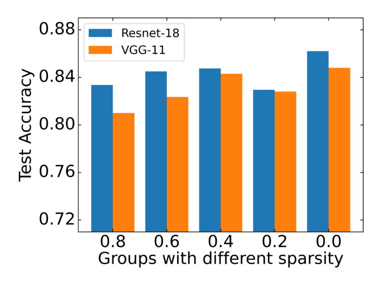
For demonstration, we run experiments on 100 nodes on CIFAR-10 dataset with Dir partition $\alpha=0.3$ and pathological partition in two settings. (i) All clients have the same capability of computing, saving, and transmitting half of the overall model. (ii) 100 nodes are grouped into 5 parts with the capability of each computing, saving and transmitting 20%, 40%, 60%, 80% and 100% parameters of the overall dense model. Since there exists not a central server here, we compare the proposed Dis-PFL with only decentralized FL baselines, D-PSGD and D-PSGD-FT. For setting (i), we implement Dis-PFL with sparsity set 0.5 for all clients, and we implement D-PSGD and D-PSGD-FT with masking half the parameters of the dense model to meet the constraints. For setting (ii), we implement Dis-PFL with assigned correspondingly sparsity in {0.0, 0.2, 0.4, 0.6, 0.8} for them. Noticeably, under setting (ii), D-PSGD and D-PSGD-FT can only be implemented with 20% model size. We choose Resnet-18 and VGG11 as the backbones.

Table 3 shows the results of our methods comparing other baselines in the client heterogeneous setting. It suggests that out approach can easily adapt to this setting. For setting (ii), we can see the performance of D-PSGD and D-PSGD-FT with only 20% parameters is relatively low due to the fact that they can not embrace the benefit of the newly developing deep models. Another interesting finding is that under a similar communication budget, compared with D-PSGD and D-PSGD-FT implemented with only 50% parameters, the proposed Dis-PFL can achieve better test accuracy. This can be attributed to the newly designed decentralized sparse training method, which better integrates the information and finds the best suitable mask.

We draw performance of each sparsity group in Figure 4. This result show that models with different sparsity, all have the ability to deal with their own tasks in the federating system no matter what the data partition or model backbone they possess. This demonstrates that our method Dis-PFL can well adapted to real life setting where heterogeneous clients may have various types of limits.

4.4 Empirical analysis of the learned sparse masks.

In order to explain how the personalized masks produced by our method can help train local personalized models for non-IID tasks, we investigate the correlation between the distance of the learned masks and task similarities. More specifically, we run experiments on a 20 nodes setting on CIFAR-10, where we partition them into 4 groups and each group shares a similar label distribution sampled with Dir(0.3). Task similarities are measured through cos-similarity between two label distributions, while the distances of the learned masks are calculated through the aligned hamming distances. Figure 5 demonstrates the correlation between them. It indicates that the personalized masks generated by our methods have the ability to accommodate to the local distribution by not only learning similar masks inside the same group with almost the same latent distributions, but also capturing similar correlations between different groups through assigning corresponding distanced masks. Noticeably, cos-similarities between label distributions and hamming distances between masks both may not best represent the true relationship among different clients. Figure 5 is only a simple and straightforward way to demonstrate the relation, deeper insights into the relationship between the learned masks and each client’s local distribution are remained for further works.

4.5 Discussion of the sparsity ratio

To discover the effects of the sparsity ratio in Dis-PFL, we run experiments on 100 clients under CIFAR-10 Dir Part with different sparsity ratios. Table 4 demonstrates that it’s challenging to find the optimal sparsity ratio. Though a higher sparsity ratio may bring more communication cost benefits, the performance degradation can not be omitted. This can be intuitively understood by the few overlap of the received masks, leading to less information exchange. On the other hand, a small sparsity ratio also performs not well since all clients share almost the same mask, mask personalization technique may not function.

This result further indicates the soundness of Theorem 1. When the sparsity ratio is small enough (all clients remain an over-parameterized network), as the sparsity ratio grows ( $\beta_{k}$ decreases), the generalization ability of the personalized model grows. However, as the traditional wisdom in machine learning (Mohri et al. 2018), there always exists a delicate balance between training error and generalization gap. Though the generalization gap can be controlled when model complexity decreases (greater sparsity), a larger training error may also lead to a bad test error. Thus, in practice, selecting a reasonable sparsity ratio (sweet point) requires significant consideration.

Table 4: Performance of Dis-PFL under different sparsity ratio.

Sparsity	0.8	0.6	0.5	0.4	0.2
Acc	83.27	84.08	85.70	84.22	84.10
Comm (MB)	89.30	178.69	223.4	268.1	357.5
FLOPS (1e12)	4.6	6.5	7.0	7.5	8.2

5 Conclusion

In this work,we propose Dis-PFL, a Decentralized sparse training based Personnalized Federated Learning approach to simultaneously tackle the data heterogeneity and client heterogeneity for personalized FL. Thanks to the newly designed decentralized sparse training technique, Dis-PFL could reduce the communication bottleneck, save local training costs, and easily adapts to the client heterogeneous setting. Furthermore, we provide theoretical and experimental understandings for the sparse masks. Extensive experiments also verify the efficacy of the proposed Dis-PFL.

Acknowledgement

This work is supported by Science and Technology Innovation 2030 –“Brain Science and Brain-like Research” Major Project (No. 2021ZD0201402 and No. 2021ZD0201405). This work is done during Rong Dai’s internship at JD Explore Academy.

References

Acar et al. (2021) Acar, D. A. E., Zhao, Y., Navarro, R. M., Mattina, M., Whatmough, P. N., and Saligrama, V. Federated learning based on dynamic regularization. In International Conference on Learning Representations, 2021.
Alistarh et al. (2017) Alistarh, D., Grubic, D., Li, J., Tomioka, R., and Vojnovic, M. Qsgd: Communication-efficient sgd via gradient quantization and encoding. Advances in Neural Information Processing Systems, 30:1709–1720, 2017.
Allen-Zhu et al. (2019) Allen-Zhu, Z., Li, Y., and Song, Z. A convergence theory for deep learning via over-parameterization. In International Conference on Machine Learning, pp. 242–252. PMLR, 2019.
Arivazhagan et al. (2019) Arivazhagan, M. G., Aggarwal, V., Singh, A. K., and Choudhary, S. Federated learning with personalization layers. arXiv preprint arXiv:1912.00818, 2019.
Balle et al. (2018) Balle, B., Barthe, G., and Gaboardi, M. Privacy amplification by subsampling: Tight analyses via couplings and divergences. In NeurIPS, 2018.
Basu et al. (2019) Basu, D., Data, D., Karakus, C., and Diggavi, S. Qsparse-local-sgd: Distributed sgd with quantization, sparsification and local computations. Advances in Neural Information Processing Systems, 32, 2019.
Bibikar et al. (2021) Bibikar, S., Vikalo, H., Wang, Z., and Chen, X. Federated dynamic sparse training: Computing less, communicating less, yet learning better. arXiv preprint arXiv:2112.09824, 2021.
Blot et al. (2016) Blot, M., Picard, D., Cord, M., and Thome, N. Gossip training for deep learning. arXiv preprint arXiv:1611.09726, 2016.
Chen et al. (2020) Chen, C., Shen, L., Huang, H., Liu, W., and Luo, Z.-Q. Efficient-adam: Communication-efficient distributed adam with complexity analysis. 2020.
Chen et al. (2021a) Chen, C., Shen, L., Huang, H., and Liu, W. Quantized adam with error feedback. ACM Transactions on Intelligent Systems and Technology (TIST), 12(5):1–26, 2021a.
Chen et al. (2021b) Chen, C., Zhang, J., Shen, L., Zhao, P., and Luo, Z. Communication efficient primal-dual algorithm for nonconvex nonsmooth distributed optimization. In International Conference on Artificial Intelligence and Statistics, pp. 1594–1602. PMLR, 2021b.
Chen & Chao (2020) Chen, H.-Y. and Chao, W.-L. Fedbe: Making bayesian model ensemble applicable to federated learning. In International Conference on Learning Representations, 2020.
Chen & Chao (2021) Chen, H.-Y. and Chao, W.-L. On bridging generic and personalized federated learning. arXiv preprint arXiv:2107.00778, 2021.
Cheng et al. (2021) Cheng, G., Chadha, K., and Duchi, J. Fine-tuning is fine in federated learning. arXiv preprint arXiv:2108.07313, 2021.
Collins et al. (2021) Collins, L., Hassani, H., Mokhtari, A., and Shakkottai, S. Exploiting shared representations for personalized federated learning. arXiv preprint arXiv:2102.07078, 2021.
Deng et al. (2020) Deng, Y., Kamani, M. M., and Mahdavi, M. Adaptive personalized federated learning. arXiv preprint arXiv:2003.13461, 2020.
Diao et al. (2020) Diao, E., Ding, J., and Tarokh, V. Heterofl: Computation and communication efficient federated learning for heterogeneous clients. In International Conference on Learning Representations, 2020.
Evci et al. (2020) Evci, U., Gale, T., Menick, J., Castro, P. S., and Elsen, E. Rigging the lottery: Making all tickets winners. In International Conference on Machine Learning, pp. 2943–2952. PMLR, 2020.
Fallah et al. (2020) Fallah, A., Mokhtari, A., and Ozdaglar, A. Personalized federated learning: A meta-learning approach. arXiv preprint arXiv:2002.07948, 2020.
Fraboni et al. (2021) Fraboni, Y., Vidal, R., Kameni, L., and Lorenzi, M. Clustered sampling: Low-variance and improved representativity for clients selection in federated learning. In International Conference on Machine Learning, pp. 3407–3416. PMLR, 2021.
Frankle & Carbin (2018) Frankle, J. and Carbin, M. The lottery ticket hypothesis: Finding sparse, trainable neural networks. In International Conference on Learning Representations, 2018.
Han et al. (2015) Han, S., Pool, J., Tran, J., and Dally, W. Learning both weights and connections for efficient neural network. Advances in Neural Information Processing Systems, 28, 2015.
Hanzely et al. (2021) Hanzely, F., Zhao, B., and Kolar, M. Personalized federated learning: A unified framework and universal optimization techniques. arXiv preprint arXiv:2102.09743, 2021.
He & Tao (2020) He, F. and Tao, D. Recent advances in deep learning theory. arXiv preprint arXiv:2012.10931, 2020.
He et al. (2019) He, F., Liu, T., and Tao, D. Control batch size and learning rate to generalize well: Theoretical and empirical evidence. In Advances in Neural Information Processing Systems, pp. 1143–1152, 2019.
He et al. (2021) He, F., Wang, B., and Tao, D. Tighter generalization bounds for iterative differentially private learning algorithms. In Uncertainty in Artificial Intelligence, pp. 802–812. PMLR, 2021.
He et al. (2016) He, K., Zhang, X., Ren, S., and Sun, J. Deep residual learning for image recognition. In Proceedings of the IEEE conference on computer vision and pattern recognition, pp. 770–778, 2016.
Hong et al. (2022) Hong, J., Wang, H., Wang, Z., and Zhou, J. Efficient split-mix federated learning for on-demand and in-situ customization. arXiv preprint arXiv:2203.09747, 2022.
Horvath et al. (2021) Horvath, S., Laskaridis, S., Almeida, M., Leontiadis, I., Venieris, S., and Lane, N. Fjord: Fair and accurate federated learning under heterogeneous targets with ordered dropout. Advances in Neural Information Processing Systems, 34, 2021.
Hsieh et al. (2020) Hsieh, K., Phanishayee, A., Mutlu, O., and Gibbons, P. The non-iid data quagmire of decentralized machine learning. In International Conference on Machine Learning, pp. 4387–4398. PMLR, 2020.
Hsu et al. (2019) Hsu, T.-M. H., Qi, H., and Brown, M. Measuring the effects of non-identical data distribution for federated visual classification. arXiv preprint arXiv:1909.06335, 2019.
Huang et al. (2022a) Huang, T., Lin, W., Shen, L., Li, K., and Zomaya, A. Y. Stochastic client selection for federated learning with volatile clients. IEEE Internet of Things Journal, 2022a.
Huang et al. (2022b) Huang, T., Liu, S., Shen, L., He, F., Lin, W., and Tao, D. Achieving personalized federated learning with sparse local models. arXiv preprint arXiv:2201.11380, 2022b.
Ivkin et al. (2019) Ivkin, N., Rothchild, D., Ullah, E., Stoica, I., Arora, R., et al. Communication-efficient distributed sgd with sketching. Advances in Neural Information Processing Systems, 32:13144–13154, 2019.
Jiang et al. (2019) Jiang, Y., Konečnỳ, J., Rush, K., and Kannan, S. Improving federated learning personalization via model agnostic meta learning. arXiv preprint arXiv:1909.12488, 2019.
Jiang et al. (2017) Jiang, Z., Balu, A., Hegde, C., and Sarkar, S. Collaborative deep learning in fixed topology networks. Advances in Neural Information Processing Systems, 30, 2017.
Khan et al. (2021) Khan, L. U., Saad, W., Han, Z., Hossain, E., and Hong, C. S. Federated learning for internet of things: Recent advances, taxonomy, and open challenges. IEEE Communications Surveys & Tutorials, 2021.
Koloskova et al. (2019) Koloskova, A., Stich, S., and Jaggi, M. Decentralized stochastic optimization and gossip algorithms with compressed communication. In International Conference on Machine Learning, pp. 3478–3487. PMLR, 2019.
Krizhevsky et al. (2009) Krizhevsky, A. et al. Learning multiple layers of features from tiny images. 2009.
Lalitha et al. (2018) Lalitha, A., Shekhar, S., Javidi, T., and Koushanfar, F. Fully decentralized federated learning. In Third workshop on Bayesian Deep Learning (NeurIPS), 2018.
Lalitha et al. (2019) Lalitha, A., Kilinc, O. C., Javidi, T., and Koushanfar, F. Peer-to-peer federated learning on graphs. arXiv preprint arXiv:1901.11173, 2019.
Li et al. (2020a) Li, A., Sun, J., Wang, B., Duan, L., Li, S., Chen, Y., and Li, H. Lotteryfl: Personalized and communication-efficient federated learning with lottery ticket hypothesis on non-iid datasets. arXiv preprint arXiv:2008.03371, 2020a.
Li et al. (2021a) Li, A., Sun, J., Zeng, X., Zhang, M., Li, H., and Chen, Y. Fedmask: Joint computation and communication-efficient personalized federated learning via heterogeneous masking. In Proceedings of the 19th ACM Conference on Embedded Networked Sensor Systems, pp. 42–55, 2021a.
Li et al. (2022) Li, S., Zhou, T., Tian, X., and Tao, D. Learning to collaborate in decentralized learning of personalized models. In Proceedings of the IEEE conference on computer vision and pattern recognition, 2022.
Li et al. (2020b) Li, T., Sahu, A. K., Zaheer, M., Sanjabi, M., Talwalkar, A., and Smith, V. Federated optimization in heterogeneous networks. Proceedings of Machine Learning and Systems, 2:429–450, 2020b.
Li et al. (2021b) Li, T., Hu, S., Beirami, A., and Smith, V. Ditto: Fair and robust federated learning through personalization. In International Conference on Machine Learning, pp. 6357–6368. PMLR, 2021b.
Lian et al. (2017) Lian, X., Zhang, C., Zhang, H., Hsieh, C.-J., Zhang, W., and Liu, J. Can decentralized algorithms outperform centralized algorithms? a case study for decentralized parallel stochastic gradient descent. Advances in Neural Information Processing Systems, 2017.
Liang et al. (2020) Liang, P. P., Liu, T., Ziyin, L., Allen, N. B., Auerbach, R. P., Brent, D., Salakhutdinov, R., and Morency, L.-P. Think locally, act globally: Federated learning with local and global representations. arXiv preprint arXiv:2001.01523, 2020.
Lim et al. (2019) Lim, H., Andersen, D. G., and Kaminsky, M. 3lc: Lightweight and effective traffic compression for distributed machine learning. Proceedings of Machine Learning and Systems, 1:53–64, 2019.
Lin et al. (2020) Lin, T., Kong, L., Stich, S. U., and Jaggi, M. Ensemble distillation for robust model fusion in federated learning. In NeurIPS, 2020.
Lin et al. (2021) Lin, T., Karimireddy, S. P., Stich, S. U., and Jaggi, M. Quasi-global momentum: Accelerating decentralized deep learning on heterogeneous data. In International Conference on Machine Learning, pp. 6654–6665. PMLR, 2021.
Liu et al. (2021a) Liu, S., Chen, T., Chen, X., Atashgahi, Z., Yin, L., Kou, H., Shen, L., Pechenizkiy, M., Wang, Z., and Mocanu, D. C. Sparse training via boosting pruning plasticity with neuroregeneration. Advances in Neural Information Processing Systems, 34, 2021a.
Liu et al. (2021b) Liu, S., Yin, L., Mocanu, D. C., and Pechenizkiy, M. Do we actually need dense over-parameterization? in-time over-parameterization in sparse training. In International Conference on Machine Learning, pp. 6989–7000. PMLR, 2021b.
Liu et al. (2022a) Liu, S., Chen, T., Chen, X., Shen, L., Mocanu, D. C., Wang, Z., and Pechenizkiy, M. The unreasonable effectiveness of random pruning: Return of the most naive baseline for sparse training. In International Conference on Learning Representations, 2022a.
Liu et al. (2022b) Liu, S., Tian, Y., Chen, T., and Shen, L. Don’t be so dense: Sparse-to-sparse gan training without sacrificing performance. arXiv preprint arXiv:2203.02770, 2022b.
Liu et al. (2018) Liu, Z., Sun, M., Zhou, T., Huang, G., and Darrell, T. Rethinking the value of network pruning. In International Conference on Learning Representations, 2018.
McMahan et al. (2017) McMahan, B., Moore, E., Ramage, D., Hampson, S., and y Arcas, B. A. Communication-efficient learning of deep networks from decentralized data. In Artificial intelligence and statistics, pp. 1273–1282. PMLR, 2017.
Mocanu et al. (2018) Mocanu, D. C., Mocanu, E., Stone, P., Nguyen, P. H., Gibescu, M., and Liotta, A. Scalable training of artificial neural networks with adaptive sparse connectivity inspired by network science. Nature communications, 9(1):1–12, 2018.
Mohri et al. (2018) Mohri, M., Rostamizadeh, A., and Talwalkar, A. Foundations of machine learning. 2018.
Mostafa & Wang (2019) Mostafa, H. and Wang, X. Parameter efficient training of deep convolutional neural networks by dynamic sparse reparameterization. In International Conference on Machine Learning, pp. 4646–4655. PMLR, 2019.
Nguyen et al. (2021) Nguyen, D. C., Ding, M., Pathirana, P. N., Seneviratne, A., Li, J., and Poor, H. V. Federated learning for internet of things: A comprehensive survey. IEEE Communications Surveys & Tutorials, 2021.
Nishio & Yonetani (2019) Nishio, T. and Yonetani, R. Client selection for federated learning with heterogeneous resources in mobile edge. In ICC 2019-2019 IEEE international conference on communications (ICC), pp. 1–7. IEEE, 2019.
Shamsian et al. (2021) Shamsian, A., Navon, A., Fetaya, E., and Chechik, G. Personalized federated learning using hypernetworks. arXiv preprint arXiv:2103.04628, 2021.
Simonyan & Zisserman (2015) Simonyan, K. and Zisserman, A. Very deep convolutional networks for large-scale image recognition. In International Conference on Learning Representations, May 2015.
Sun et al. (2021) Sun, T., Li, D., and Wang, B. Decentralized federated averaging. arXiv preprint arXiv:2104.11375, 2021.
T Dinh et al. (2020) T Dinh, C., Tran, N., and Nguyen, T. D. Personalized federated learning with moreau envelopes. Advances in Neural Information Processing Systems, 33, 2020.
Vahidian et al. (2021) Vahidian, S., Morafah, M., and Lin, B. Personalized federated learning by structured and unstructured pruning under data heterogeneity. arXiv preprint arXiv:2105.00562, 2021.
Voigt & Von dem Bussche (2017) Voigt, P. and Von dem Bussche, A. The eu general data protection regulation (gdpr). A Practical Guide, 1st Ed., Cham: Springer International Publishing, 10:3152676, 2017.
Wang et al. (2020) Wang, H., Yurochkin, M., Sun, Y., Papailiopoulos, D., and Khazaeni, Y. Federated learning with matched averaging. In International Conference on Learning Representations, 2020.
Warnat-Herresthal et al. (2021) Warnat-Herresthal, S., Schultze, H., Shastry, K. L., Manamohan, S., Mukherjee, S., Garg, V., Sarveswara, R., Händler, K., Pickkers, P., Aziz, N. A., et al. Swarm learning for decentralized and confidential clinical machine learning. Nature, 594(7862):265–270, 2021.
Wen et al. (2017) Wen, W., Xu, C., Yan, F., Wu, C., Wang, Y., Chen, Y., and Li, H. Terngrad: Ternary gradients to reduce communication in distributed deep learning. Advances in Neural Information Processing Systems, 30, 2017.
Wu & He (2018) Wu, Y. and He, K. Group normalization. In Proceedings of the European conference on computer vision (ECCV), pp. 3–19, 2018.
Yu et al. (2019) Yu, Y., Wu, J., and Huang, J. Exploring fast and communication-efficient algorithms in large-scale distributed networks. In The 22nd International Conference on Artificial Intelligence and Statistics, pp. 674–683. PMLR, 2019.
Yuan et al. (2021) Yuan, Y., Chen, R., Sun, C., Wang, M., Hua, F., Yi, X., Yang, T., and Liu, J. Defed: A principled decentralized and privacy-preserving federated learning algorithm. arXiv preprint arXiv:2107.07171, 2021.
Zhang et al. (2022) Zhang, L., Shen, L., Ding, L., Tao, D., and Duan, L.-Y. Fine-tuning global model via data-free knowledge distillation for non-iid federated learning. arXiv preprint arXiv:2203.09249, 2022.
Zhang et al. (2020) Zhang, M., Sapra, K., Fidler, S., Yeung, S., and Alvarez, J. M. Personalized federated learning with first order model optimization. In International Conference on Learning Representations, 2020.
Zhu et al. (2022) Zhu, T., He, F., Zhang, L., Niu, Z., Song, M., and Tao, D. Topology-aware generalization of decentralized sgd. In International Conference on Machine Learning, 2022.
Zou & Gu (2019) Zou, D. and Gu, Q. An improved analysis of training over-parameterized deep neural networks. Advances in Neural Information Processing Systems, 32:2055–2064, 2019.

Appendix

Appendix A More details on algorithm implementation

A.1 Algorithm 2

We present the local mask searching method as in Algorithm 2 here.

Algorithm 2 Local mask searching

Input:

\boldsymbol{w}_{k,t+1}

and corresponding mask

\boldsymbol{m}_{k,t}

Output: New mask

\boldsymbol{m}_{k,t+1}

Compute current prune rate

\alpha_{t}

using cosine annealing principle with initial pruning rate

\alpha_{0}

Sample a batch of local data and do loss backward to get the dense gradient

g({w}_{k,t+1})

for layer

j

\in

J

do do

Update mask

m^{j}_{k,t+\frac{1}{2}}

by zeroing out

\alpha_{t}

-proportion of weights with magnitude pruning

Update mask

m^{j}_{k,t+1}

via recovering weights with gradient information

g({w}_{k,t+1})

end for

Get new mask

m_{k,t+1}

Appendix B Experiments

In this section, we provide more details of our experiments and more extensive experimental results to compare the performance of the proposed Dis-PFL against other baselines.

B.1 Datasets

We use CIFAR-10 (10 classes, 5000 training samples each), CIFAR-100 (100 classes, 500 training samples each), and Tiny-Imagenet (200 classes, 500 training samples each) for the experiments. We use two non-IID partition methods to split the training data in our implementation. One is based on the Dirichlet distribution on the label ratios to ensure uneven label distributions among devices as in (Hsu et al. 2019), a smaller $\alpha$ indicates higher data heterogeneity. The other is called pathological partition, which means only assigning samples of specific classes for each client. To simulate the personalized FL setting, each client’s testing data has the same proportion of labels as its training data, and the total number of the testing set is set to 100 for all partitions.

B.2 Model Architectures

We follow the pytorch’s implementation of ResNet18 (He et al. 2016) and VGG11 (Simonyan & Zisserman 2015) to do all the evaluations. Since batch-norm may have a detrimental effect on federated learning (Hsieh et al. 2020), we replace all the batch-norm layers in ResNet18 and VGG11 with group-norm layers (Wu & He 2018).

B.3 Hyper-Parameters

We use SGD optimizer for all methods with weighted decayed parameter 0.0005. For all the methods except Ditto, local epochs are fixed to 5. For Ditto, in order to ensure a fair comparison, each client performs 3 epochs for training the local model and 2 epochs for training the global model. The learning rate is initialized with 0.1 and decayed with 0.998 after each communication round. The batch size is fixed to 128 for all the experiments. We run 500 global communication rounds for CIFAR-10, CIFAR-100, and 300 for Tiny-Imagenet. The setting of hype-parameters also impacts the generalizability (He et al. 2019).

B.4 More details about baselines

Local is the direct solution to the personalized federated learning problem. Each client only performs SGD on their own data. For the sake of consistency, we take 5 epochs of local training as one communication round. FedAvg (McMahan et al. 2017) is the most widely studied FL method. The vanilla weighted average is used to enable all the clients to collaboratively train a global model. FedAvg-FT(Cheng et al. 2021) is a simple method by doing some fine-tuning steps with local data after acquiring the global model but shown to be competitive against various personalized federated learning specific methods. Ditto (Li et al. 2021b) achieves personalization via trade-off between the global model and local objectives. Specifically, within each communication round, each client first trains the global model (similarly aggregated as in FedAvg) on its local empirical risk. And then additionally trains its local model based on a loss function combining its local empirical loss and the proximal term towards the global model. FOMO (Zhang et al. 2020) trains personalized models using neighbors’ gradient information to infer how much a client can benefit from another’s model and thus get the adaptive mixing weights for personalization. SubFedAvg (Vahidian et al. 2021) maintains personalized sub-networks for each user. The overall training process follows a dense-to-spare training rule, the client’s local model starts from a fully dense model, and is iteratively pruned as the training progresses. D-PSGD (Lian et al. 2017) is a classic decentralized parallel stochastic gradient descent method proposed to reach a consensus model on a decentralized network. Each node first averages the local variables with the received models and then updates it using the local stochastic gradient. To extend it to the federated learning scenarios, following (Sun et al. 2021), we take several epochs of local training instead of one iteration for each local client. We also extend it to D-PSGD-FT following the idea of FedAvg-FT, several steps of local fine-tuning are done to further personalize the global consensus model towards heterogeneous clients.

B.5 More experiments results

B.5.1 Convergence speed

We demonstrate the needed communication rounds for each method to reach a target accuracy as follows. Results for CIFAR-10 are in Table 5, while results for CIFAR-100 in Table 6 and Tiny-Imagenet in Table 7.

Table 5: Averaged needed communication rounds for each method to a target accuracy on CIFAR-10 dataset.

Methods	Dir partition			Pathological partition
Methods	Acc@60	Acc@70	Acc@80	Acc@50	Acc@80	Acc@85
FedAvg	159	267	>500	388	>500	>500
D-PSGD	139	236	>500	391	>500	>500
Ditto	176	375	>500	21	138	256
FOMO	204	>500	>500	3	45	129
SubFedAvg	67	115	>500	33	99	181
Dis-PFL	59	144	301	3	33	81

Table 6: Averaged needed communication rounds for each method to a target accuracy on CIFAR-100 dataset.

Methods	Dir partition			Pathological partition
Methods	Acc@25	Acc@40	Acc@50	Acc@30	Acc@50	Acc@60
FedAvg	195	454	>500	393	>500	>500
D-PSGD	157	437	>500	326	>500	>500
Ditto	201	>500	>500	136	393	>500
FOMO	171	>500	>500	23	223	>500
SubFedAvg	161	228	>500	148	202	377
Dis-PFL	64	231	393	29	159	293

Table 7: Averaged needed communication rounds for each method to a target accuracy on Tiny-Imagenet dataset.

Methods	Dir partition			Pathological partition
Methods	Acc@05	Acc@10	Acc@15	Acc@05	Acc@10	Acc@20
FedAvg	92	206	>300	89	>300	>300
D-PSGD	61	141	>300	66	185	>300
Ditto	39	137	261	19	84	211
FOMO	168	>300	>300	2	>300	>300
SubFedAvg	80	201	>300	88	222	>300
Dis-PFL	13	58	195	3	18	63

B.5.2 Different topology

Similar to Table 2, we also record performances of each method under different decentralized topology in Table 8 for CIFAR-100 and Table 9 for Tiny-Imagenet.

Table 8: Table illustrating performance compared with methods in decentralized communication protocols on CIFAR-100.

Dataset	Topology	Method	Dir Part Acc	Path Part Acc	Comm (MB)	FLOPS (1e12)
CIFAR-100	Seperate	Local	29.23 $\pm$ 0.2	52.46 $\pm$ 0.2	-	8.3
	Ring	D-PSGD	17.52 $\pm$ 0.2	10.62 $\pm$ 0.5	89.7	8.3
		D-PSGD-FT	32.61 $\pm$ 0.3	51.67 $\pm$ 0.2	89.7	8.3
		Dis-PFL(ours)	33.13 $\pm$ 0.2	52.08 $\pm$ 0.3	44.8
	Fully-connected	D-PSGD	43.18 $\pm$ 0.4	36.81 $\pm$ 0.4	4442.2	8.3
		D-PSGD-FT	53.40 $\pm$ 0.2	68.23 $\pm$ 0.2	4442.2	8.3
		Dis-PFL(ours)	52.85 $\pm$ 0.2	72.97 $\pm$ 0.5	2222.0	7.0

Table 9: Table illustrating performance compared with methods in decentralized communication protocols on Tiny-Imagenet.

Dataset	Topology	Method	Dir Part Acc	Path Part Acc	Comm (MB)	FLOPS (1e12)
Tiny-Imagenet	Seperate	Local	6.76 $\pm$ 0.2	17.68 $\pm$ 0.3	-	6.7
	Ring	D-PSGD	3.63 $\pm$ 0.4	3.02 $\pm$ 0.5	90.1	66.6
		D-PSGD-FT	9.66 $\pm$ 0.2	19.72 $\pm$ 0.4	90.1	66.6
		Dis-PFL(ours)	9.60 $\pm$ 0.2	20.17 $\pm$ 0.2	45.0	54.5
	Fully-connected	D-PSGD	12.92 $\pm$ 0.3	11.58 $\pm$ 0.3	4462.5	66.6
		D-PSGD-FT	16.52 $\pm$ 0.2	29.76 $\pm$ 0.3	4462.5	66.6
		Dis-PFL(ours)	17.10 $\pm$ 0.3	31.93 $\pm$ 0.2	2229.8	54.5

B.6 Extended experiments on random clients dropping settings

It’s common to see that clients or the server may fail to all take part in every communication round in the federated system. A server malfunction may hurt the overall system, thus leading to the failed operation of the whole system. However, this weakness can be alleviated in the decentralized setting, since one or more clients drop this round may not hurt the overall training process. We here conduct the dropped clients experiments on Dis-PFL to demonstrate the robustness to random client dropping of the proposed method. The experiments are conducted on CIFAR-10 with 100 clients under Dir partition.

As shown in Figure 6, our proposed Dis-PFL can provide fairly decent personalized models for each device participating in the federation system compared with local training, regardless of the device dropping probability. Admittedly, as the probability of device disconnection increases, the convergence speed of the Dis-PFL may slow down, and it may also affect the final personalized result. Nevertheless, our proposed decentralized personalization algorithm is still more robust than the centralized personalization algorithm since if the server drops in a certain communication round, the entire centralized system cannot work at all.

Appendix C Proof of Theorem 1

This section demonstrates the proof of Theorem 1 in detail. We first clarify the notations and preliminaries in C.1 and present some key lemmas in C.2 and finally present the proof in C.3.

C.1 Notations and Preliminaries

$S=\{(x_{1},y_{1}),\ldots,(x_{N},y_{N})|x_{i}\in\mathcal{X}\subset\mathbb{R}^{d_{X}},$ $y_{i}\in\mathcal{Y}\subset\mathbb{R}^{d_{Y}},i=1,\ldots,N\}$ is a training sample set, where $x_{i}$ is the $i$ -th feature, $y_{i}$ is the corresponding label, and $d_{X}$ and $d_{Y}$ are the dimensions of the feature and the label, respectively. For the brevity, we define $z_{i}=(x_{i},y_{i})$ . We also define random variables $Z=(X,Y)$ , such that all $z_{i}=(x_{i},y_{i})$ are independent and identically distributed (i.i.d.) observations of the variable $Z=(X,Y)\in\mathcal{Z},~Z\sim\mathcal{D}$ , where $\mathcal{D}$ is the data distribution.

For a machine learning algorithm $\mathcal{A}$ , it learns a hypothesis $\mathcal{A}(S)$ , $\mathcal{A}(S)\in\mathcal{H}\subset\mathcal{Y}^{\mathcal{X}}=\{f:\mathcal{X}\to\mathcal{Y}\}$ .

The expected risk $\mathcal{R}_{D}(\mathcal{A}(S))$ and empirical risk $\hat{\mathcal{R}}_{\mathcal{S}}(\mathcal{A}(S))$ of the algorithm $\mathcal{A}$ are defined as follows,

	$\displaystyle\mathcal{R}_{\mathcal{D}}(\mathcal{A}(S))=\mathbb{E}_{z\sim\mathcal{D}}\ell(\mathcal{A}(S),z),$
	$\displaystyle\hat{\mathcal{R}}_{S}(\mathcal{A}(S))=\frac{1}{N}\sum_{i=1}^{N}\ell(\mathcal{A}(S),z_{i}),$

where $\ell:\mathcal{H}\times\mathcal{Z}\to\mathbb{R}^{+}$ is the loss function.

Definition 1 (Generalization bound).

The generalization error is defined as the difference between the expected risk and empirical risk,

\operatorname{Gen}_{S,\mathcal{A}(S)}\overset{\triangle}{=}\mathcal{R}_{\mathcal{D}}(\mathcal{A}(S))-\hat{\mathcal{R}}_{S}(\mathcal{A}(S)),

whose upper bound is called the generalization bound.

Definition 2 (Differential Privacy).

A stochastic algorithm $\mathcal{A}$ is called ( $\varepsilon,\delta$ )-differentially private if for any hypothesis subset $\mathcal{H}_{0}\subset\mathcal{H}$ and any neighboring sample set pair $S$ and $S^{\prime}$ which differ by only one example (called $S$ and $S^{\prime}$ adjacent), we have

\log\left[\frac{\mathbb{P}_{\mathcal{A}(S)}(\mathcal{A}(S)\in\mathcal{H}_{0})-\delta}{\mathbb{P}_{\mathcal{A}(S^{\prime})}(\mathcal{A}(S^{\prime})\in\mathcal{H}_{0})}\right]\leq\varepsilon.

The algorithm $\mathcal{A}$ is also called $\varepsilon$ -differentially private, if it is $(\varepsilon,0)$ -differentially private.

Definition 3 (Multi-Sample-Set Learning Algorithms).

Suppose the training sample set $S$ with size $kN$ is separated to $k$ sub-sample-sets $S_{1},\ldots,S_{k}$ , each of which has the size of $N$ . In another word, $S$ is formed by $k$ sub-sample-sets as

S=(S_{1},\ldots,S_{k}).

The hypothesis $\mathcal{B}(S)$ learned by multi-sample-set algorithm $\mathcal{B}$ on dataset $S$ is defined as follows,

\mathcal{B}:\mathcal{Z}^{k\times N}\mapsto\mathcal{H}\times\{1,\ldots,k\},~\mathcal{B}(S)=\left(h_{\mathcal{B}(S)},i_{\mathcal{B}(S)}\right).

C.2 Key Lemmas

Lemma 1 (c.f. Theorem 9 Balle et al. 2018).

This lemma provide bound of differential privacy parameters after sub-sampling uniformly without replacement. Let $\mathcal{M}^{o}:\mathcal{Z}^{m}\mapsto\Delta\mathcal{H}$ be any mechanism preserving $(\varepsilon,\delta)$ differential privacy. Let $\mathcal{M}^{wo}:\mathcal{Z}^{N}\mapsto\Delta\mathcal{Z}^{m}$ be the uniform sub-sampling without replacement mechanism. Then mechanism $\mathcal{M}^{o}\circ\mathcal{M}^{wo}$ satisfy $(\log(1+(m/N)(e^{\varepsilon}-1)),m\delta/N)$ differential privacy.

Lemma 2 (c.f. Theorem 4 He et al. 2021).

This lemma gives the relationship between one step privacy preserving methods and iterative machine learning methods. Suppose an iterative machine learning algorithm $\mathcal{A}$ has $T$ steps: $\left\{W_{i}(S)\right\}_{i=1}^{T}$ . Specifically, we define the $i$ -th iterator as follows,

\mathcal{M}_{i}:(W_{i-1}(S),S)\mapsto W_{i}(S).

Assume that $W_{0}$ is the initial hypothesis (which does not depend on $S$ ). If for any fixed $W_{i-1}$ , $\mathcal{M}_{i}(W_{i-1},S)$ is $\varepsilon_{i}$ -differentially private, then $\left\{W_{i}\right\}_{i=0}^{T}$ is ( $\varepsilon^{\prime}$ , $\delta^{\prime}$ )-differentially private that

\varepsilon^{\prime}=\sqrt{2\log\left(\frac{1}{\delta^{\prime}}\right)\left(\sum\limits_{i=1}^{T}\varepsilon_{i}^{2}\right)}+\sum\limits_{i=1}^{T}\varepsilon_{i}\frac{e^{\varepsilon_{i}}-1}{e^{\varepsilon_{i}}+1},

	$\displaystyle\delta^{\prime}=$	$\displaystyle e^{-\frac{\varepsilon^{\prime}+T\varepsilon}{2}}\left(\frac{1}{1+e^{\varepsilon}}\left(\frac{2T\varepsilon}{T\varepsilon-\varepsilon^{\prime}}\right)\right)^{T}\left(\frac{T\varepsilon+\varepsilon^{\prime}}{T\varepsilon-\varepsilon^{\prime}}\right)^{-\frac{\varepsilon^{\prime}+T\varepsilon}{2\varepsilon}}-\left(1-\frac{\delta}{1+e^{\varepsilon}}\right)^{T}$
		$\displaystyle+2-\left(1-e^{\varepsilon}\frac{\delta}{1+e^{\varepsilon}}\right)^{\left\lceil\frac{\varepsilon^{\prime}}{\varepsilon}\right\rceil}\left(1-\frac{\delta}{1+e^{\varepsilon}}\right)^{T-\left\lceil\frac{\varepsilon^{\prime}}{\varepsilon}\right\rceil}.$

Lemma 3 (c.f. Theorem 1 He et al. 2021).

This lemma gives a high-probability generalization bound for any ( $\varepsilon,\delta$ )-differentially private machine learning algorithm. Suppose algorithm $\mathcal{A}$ is ( $\varepsilon,\delta$ )-differentially private, the training sample size $N\geq\frac{2}{\varepsilon^{2}}\ln\left(\frac{16}{e^{-\varepsilon}\delta}\right)$ , and the loss function $\|l\|_{\infty}\leq 1$ . Then, for any data distribution $\mathcal{D}$ over data space $\mathcal{Z}$ , we have the following inequality,

\mathbb{P}\left[\left|\hat{\mathcal{R}}_{S}(\mathcal{A}(S))-\mathcal{R}(\mathcal{A}(S))\right|<9\varepsilon\right]>1-\frac{e^{-\varepsilon}\delta}{\varepsilon}\ln\left(\frac{2}{\varepsilon}\right).

C.3 Main proof

Proof.

The main proof can be seen as acquiring generalization bound through the lens of differential privacy. The proof skeleton can be concluded in three stages: (1) We first take a global view of the proposed algorithm Dis-PFL and thus classify it as an iterative machine learning algorithm. (2) We then calculate the differential privacy of each step in the algorithm. (3) Extend it to iterative situations and acquire the final result through the bridges provided in (He et al. 2021).

First, let us take a global view of the overall decentralized training process. We can assume that the initial consensus model derived using the model fusion approach in the newly designed decentralized sparse training technique is the same for all clients. Afterward, each client multiplies the personalized mask with this consensus model to get the specific initial model for them to further operate local sparse training and mask searching. Thus, a global consensus model $\boldsymbol{w}$ always exists during the overall training process. The proportion of remaining parameters for this model $\beta$ is inferred from the aggregation of all the local clients with $\beta_{k}$ remaining params.

For simplicity, we define $W_{t}$ as the virtual consensus model at iteration $t$ . Then the decentralized learning paradigm can be seen as iteratively optimize $W$ using partial gradient information (due to the sparse mask) on each client $k$ . We also denote $\mathcal{N}(0,\sigma^{2}\mathbb{I})$ as a Gaussian noise, where $\sigma$ is the Gaussian noise variance. We define $\tau$ as the mini-batch size and overall iteration steps as $T$ . We assume the computed gradient of the loss function $\mathcal{L}$ is bounded, and the diameter of the gradient space is defined as $D_{g}\overset{\triangle}{=}\max_{W,z,z^{\prime}}\|\nabla\ell(z,W)-\nabla\ell(z^{\prime},W)\|$ . We also denote $G_{\mathcal{B}}(W)\overset{\triangle}{=}\frac{1}{\|\mathcal{B}\|}\sum_{z\in\mathcal{B}}g(z,W)$ as the mean of $g$ over $\mathcal{B}$ for brevity. We also use $\boldsymbol{p}$ as the probability density, with $\boldsymbol{p}^{V}$ the probability density conditional on any random variable $V$ .

Then we calculate the differential privacy of each step. Recall Algorithm 1, line 9-13 denotes the local training process, the gradient information, $\bigtriangledown_{\widetilde{\boldsymbol{w}}_{k,t,\tau}}$ is calculated on the subset of local data. However, in real federating system, for privacy concerns, additive Gaussian noise sample is also used to enhance privacy. Line 10 in Algorithm 1 is equivalent to uniformly sampling a mini-batch $\mathcal{I}_{t}$ from index set $[N]$ with size $\tau$ without replacement and letting $\mathcal{B}_{t}=S_{\mathcal{I}_{t}}$ . Furthermore, for fixed $W_{t-1}$ , $\mathcal{I}$ , and any two adjacent sample sets $S$ and $S^{\prime}$ , we have

	$\displaystyle\frac{\boldsymbol{p}^{S,\mathcal{I}_{t}}(W_{t}=W\|W_{t-1})}{\boldsymbol{p}^{S^{\prime},\mathcal{I}_{t}}(W_{t}=W\|W_{t-1})}$	$\displaystyle=\frac{\boldsymbol{p}^{S,\mathcal{I}_{t}}(\eta_{t}(G_{S_{\mathcal{I}}}(W_{t-1})+\mathcal{N}(0,\sigma^{2}\mathbb{I}))=W-W_{t-1})}{\boldsymbol{p}^{S^{\prime},\mathcal{I}_{t}}(\eta_{t}(G_{S^{\prime}_{\mathcal{I}}}(W_{t-1})+\mathcal{N}(0,\sigma^{2}\mathbb{I}))=W-W_{t-1})}$		(6)
		$\displaystyle=\frac{\boldsymbol{p}^{\mathcal{I}_{t},W_{t-1}}(\mathcal{N}(0,\sigma^{2}\mathbb{I})=W^{\prime})}{\boldsymbol{p}^{S,S^{\prime},\mathcal{I}_{t},W_{t-1}}(G_{S^{\prime}_{\mathcal{I}}}(W_{t-1})-G_{S_{\mathcal{I}}}(W_{t-1})+\mathcal{N}(0,\sigma^{2}\mathbb{I})=W^{\prime})},$		(6)

where $\eta_{t}W^{\prime}=W-W_{t-1}-\eta_{t}G_{S_{\mathcal{I}}}(W_{t-1})$ . Therefore, when consider the additive Gaussian noise into consideration, if $W\sim W_{t-1}+\eta_{t}(G_{S_{\mathcal{I}}}(W_{t-1})+\mathcal{N}(0,\sigma\mathbb{I}))$ , then $W^{\prime}\sim G_{S_{\mathcal{I}}}(W_{t-1})+\mathcal{N}(0,\sigma\mathbb{I})$ .

For simplicity, according to the definition of differential privacy, we define

D_{p}^{S,S^{\prime},\mathcal{I}_{t},W_{t-1}}(W^{\prime})=\log\frac{\boldsymbol{p}^{\mathcal{I}_{t},W_{t-1}}(\mathcal{N}(0,\sigma^{2}\mathbb{I})=W^{\prime})}{\boldsymbol{p}^{S,S^{\prime},\mathcal{I}_{t},W_{t-1}}(G_{S^{\prime}_{\mathcal{I}}}(W_{t-1})-G_{S_{\mathcal{I}}}(W_{t-1})+\mathcal{N}(0,\sigma^{2}\mathbb{I})=W^{\prime})},

(7)

which by the definition of Gaussian distribution further leads to

	$\displaystyle D_{p}(W^{\prime})=$	$\displaystyle-\frac{\\|W^{\prime}\\|^{2}}{2\sigma^{2}}+\frac{\\|W^{\prime}-G_{S^{\prime}_{\mathcal{I}}}(W_{t-1})+G_{S_{\mathcal{I}}}(W_{t-1})\\|^{2}}{2\sigma^{2}}$		(8)
	$\displaystyle=$	$\displaystyle\frac{2\langle W^{\prime},-G_{S^{\prime}_{\mathcal{I}}}(W_{t-1})+G_{S_{\mathcal{I}}}(W_{t-1})\rangle+\\|G_{S^{\prime}_{\mathcal{I}}}(W_{t-1})-G_{S_{\mathcal{I}}}(W_{t-1})\\|^{2}}{2\sigma^{2}}.$		(8)

Denote $-G_{S^{\prime}_{\mathcal{I}}}(W_{t-1})+G_{S_{\mathcal{I}}}(W_{t-1})$ as $\mathbf{v}$ . By the definition of $D_{g}$ (the diameter of the gradient space), remember the local training step is operated on each client with different sparsity and different sparse masks, the corresponding computed gradient is thus bounded by $\beta_{k}D_{g}$ . Again by the definition of $\beta$ , which is the proportion of the remaining parameters of the aggregated global model $W$ , we can thus further bound the gradient computed on each client by $\beta D_{g}$ .

Then we have

\|\mathbf{v}\|<\frac{1}{\tau}\beta D_{g}.

(9)

On the other hand, since $\langle\mathbf{v},W^{\prime}\rangle\sim\mathcal{N}(0,\|\mathbf{v}\|^{2}\sigma^{2})$ , by Chernoff Bound technique, we have

	$\displaystyle\mathbb{P}\left(\langle\mathbf{v},W^{\prime}\rangle\geq\frac{\sqrt{2}\beta D_{g}\sigma}{\tau}\sqrt{\log\frac{1}{\delta}}\right)$	$\displaystyle\leq\mathbb{P}\left(\langle\mathbf{v},W^{\prime}\rangle\geq\sqrt{2}\\|\mathbf{v}\\|\sigma\sqrt{\log\frac{1}{\delta}}\right)$		(10)
		$\displaystyle\leq\min_{t}e^{-\sqrt{2}t\\|\mathbf{v}\\|\sigma\sqrt{\log\frac{1}{\delta}}}\mathbb{E}(e^{t\langle\mathbf{v},W^{\prime}\rangle}).$		(10)

For brevity, we define

\delta=\min_{t}e^{-\sqrt{2}t\|\mathbf{v}\|\sigma\sqrt{\log\frac{1}{\delta}}}\mathbb{E}(e^{t\langle\mathbf{v},W^{\prime}\rangle}).

(11)

Therefore, with probability at least $1-\delta$ with respect to $W^{\prime}$ , we have that

D_{p}(W^{\prime})\leq\frac{\sqrt{2}\beta D_{g}\sigma\frac{1}{\tau}\sqrt{\log\frac{1}{\delta}}+\frac{1}{\tau^{2}}\beta D_{g}^{2}}{2\sigma^{2}}.

(12)

Combining Lemma 1, we can have that the each step in Algorithm 1 is ( $\tilde{\varepsilon},\frac{\tau}{N}\delta$ )-differentially private, where $\tilde{\varepsilon}$ is defined as

\tilde{\varepsilon}=\log\left(\frac{N-\tau}{N}+\frac{\tau}{N}\exp\left(\frac{\sqrt{2}\beta D_{g}\sigma\frac{1}{\tau}\sqrt{\log\frac{1}{\delta}}+\frac{1}{\tau^{2}}\beta^{2}D_{g}^{2}}{2\sigma^{2}}\right)\right).

(13)

Applying Lemma 2, we can conclude the differentially private guarantee ( $\varepsilon^{\prime},\delta^{\prime}$ ) for the iterative steps.

Finally, combining Lemma 3 with ( $\varepsilon^{\prime},\delta^{\prime}$ ) finish the proof. ∎

DisPFL: Towards Communication-Efficient Personalized Federated Learning via Decentralized Sparse Training

Abstract

Keywords:

1 Introduction

2 Related Work

3 Dis-PFL algorithm

3.1 Problem formulation

3.2 Algorithm

3.3 Generalization analysis

Theorem 1.

Remark 1.

4 Experiments

4.1 Experiment Setup

Dataset and Data partition.

Baselines.

Communication protocol.

Configurations.

4.2 Main experiments evaluation

Test accuracy of the personalized model.

Communication cost and local training cost.

Convergence speed.

4.3 Experiments on client heterogeneous setting

4.4 Empirical analysis of the learned sparse masks.

4.5 Discussion of the sparsity ratio

5 Conclusion

Acknowledgement

References

Appendix A More details on algorithm implementation

A.1 Algorithm 2

Appendix B Experiments

B.1 Datasets

B.2 Model Architectures

B.3 Hyper-Parameters

B.4 More details about baselines

B.5 More experiments results

B.5.1 Convergence speed

B.5.2 Different topology

B.6 Extended experiments on random clients dropping settings

Appendix C Proof of Theorem 1

C.1 Notations and Preliminaries

Definition 1 (Generalization bound).

Definition 2 (Differential Privacy).

Definition 3 (Multi-Sample-Set Learning Algorithms).

C.2 Key Lemmas

Lemma 1 (c.f. Theorem 9 Balle et al. 2018).

Lemma 2 (c.f. Theorem 4 He et al. 2021).

Lemma 3 (c.f. Theorem 1 He et al. 2021).

C.3 Main proof

Proof.

DisPFL: Towards Communication-Efficient Personalized Federated Learning
via Decentralized Sparse Training