Spectral Recognition of Magnetic Nanoparticles with Artificial Neural NetworksPreprint: AIP/123-QED
Abstract
Ferromagnetic resonance (FMR) spectroscopy is a powerful method for quantifying internal magnetic anisotropy fields in nanoparticles, which is important in a wide range of biomedical and storage applications. The interpretation of FMR spectra, however, can only be achieved with the use of an appropriate model, and no inverse methods are available to extract internal fields from FMR spectra. Here, we present the use of artificial neural networks for spectral recognition, i.e., to identify the internal magnetic anisotropy field from the FMR spectrum. We trained two different types of networks, a convolutional neural network and a multi-layer perceptron, by feeding the networks pre-computed FMR spectra labeled with the corresponding anisotropy fields. Testing of the trained networks with unseen spectra showed that they successfully predict the correct anisotropy fields and, surprisingly, the networks performed well for data that was beyond their training range. These results show the promise of using artificial neural networks for accelerated high-throughput analysis of magnetic materials and nanostructures; for example they could serve in automatizing and optimizing exploration missions where nanomagnetic signals are often used as proxies.
Keywords:
magnetic nanoparticle, ferromagnetic resonance, magnetic anisotropy, artificial neural networkI Introduction
The ability to quantify the magnetic properties of nanoparticles and their assemblies is essential in enabling the progress of numerous applications, particularly in biomedicine Pankhurst et al. 2003; McBain et al. 2008; Colombo et al. 2012; Dürr et al. 2013; Périgo et al. 2015; Ruta et al. 2015; Chandrasekharan et al. 2018; Materón et al. 2021 and bio-geological exploration Weiss et al. 2004; Gehring et al. 2011; Blattmann et al. 2020. Specifically, it is important to understand the association between internal anisotropy fields and inter-particle interaction fields with the performance and overall response of the nanoparticles to external stimuli Myrovali et al. 2016; Moreno et al. 2020; Slay et al. 2021, and this requires techniques that enable the quantification of internal magnetic fields on the nanoscale. One of the most powerful techniques for the investigation of magnetic nanoparticles is ferromagnetic resonance spectroscopy (FMR) Kittel 1948, because it can provide selective and quantitative information about the magnetic anisotropy fields. The interpretation of FMR spectra, however, requires the appropriate theoretical model in order to link the material parameters, i.e., the internal anisotropy fields, to the shape of the FMR spectrum Kittel 1948; Shapiro 1966; von Bardeleben et al. 2020. Here, we show that artificial neural networks can be trained to identify material parameters from the FMR spectrum of powder samples, thus providing a novel way for high throughput spectral recognition of magnetic nanoparticles.
In an FMR experiment, a bias field is applied to magnetize the sample and a microwave field , with a frequency in the range 10 – 100 GHz, is applied orthogonally to the bias field. Typically, the frequency of the microwave is fixed and the spectrum is recorded, while sweeping the bias field, by measuring the out-of-phase susceptibility , which is a measure of dissipation, i.e., how much of the microwave energy the sample absorbs. With increasing strength of , the Larmor precession frequency of the magnetic moments in the sample increases, and when the precession frequency matches the frequency of the microwave field, resonance occurs and the sample absorbs microwave radiation at the maximum. In ferromagnetic materials, the Larmor frequency depends on the effective field in the sample, which consists of both external and internal fields, and the resonance field therefore contains information about the internal fields in the material: if the internal anisotropy field is in the same direction as the bias field, a smaller bias field is needed to accomplish resonance, and reversely, if the anisotropy field works against the bias field, a higher bias field is needed for resonance. Given that, one can quantify the magnetic anisotropy of single ferromagnetic crystals by measuring the resonance field as a function of the crystal orientation. In powder samples, e.g. ensembles of randomly oriented nanoparticles, one records the resonances at each orientation with a single measurement, and the FMR spectrum is a convolution of multiple resonances. Numerous FMR investigations of magnetic nanoparticles have provided insight to the modeling of FMR spectra using forward modeling de Biasi and Devezas 1978; Kliava and Berger 1999; Berger et al. 2000; Berger et al. 2001; Sukhov et al. 2008; de Biasi et al. 2003; de Biasi et al. 2013; Raikher and Stepanov 1994; Poperechny and Raikher 2016; Noginova et al. 2007; Noginova et al. 2008; Gazeau et al. 1999; Schmool and Schmaltz 2000; Li et al. 2009; Usselman et al. 2012, for example by solving the Landau-Lifshitz-Gilbert (LLG) equation of motion Kliava and Berger 1999; Berger et al. 2000; Berger et al. 2001; Sukhov et al. 2008 or by solving the athermal resonance equation Smit and Beljers 1955; Suhl 1955; Baselgia et al. 1988. Despite having a solid foundation for calculating FMR spectra, the direct comparison between theory and experiment remains challenging because it constitutes an inverse problem. Recent advances in computational methods can provide solutions to this problem. For example, the use a genetic algorithm to decode FMR spectra of nanoparticle assemblies was shown to be promising, but for a limited range of systems Usov and Serebryakova 2022. Artificial neural networks (NN) Rosenblatt 1962; LeCun et al. 2015 have recently been rapidly advancing computational techniques with very promising performances. In magnetism, NN have been shown to predict the response of the magnetization to an external field Kovacs et al. 2019, to reproduce hysteresis based on the Preisach model Makaveev et al. 2001; Antonio et al. 2021 and based on experimental data Yekta et al. 2019, and they also showed promise in solving inverse problems in magnetostatics and micromagnetics Kovacs et al. 2022.
Here, we show that artificial neural networks can determine anisotropy fields in magnetic nanoparticles by associating FMR spectra with material parameters, given the appropriate training with data produced by a Stoner-Wohlfarth-type model Charilaou et al. 2011; Charilaou 2017. Below, we discuss the theoretical model of single-domain magnetic nanoparticles with uniaxial symmetry, which is a good approximation for a wide range of real systems. Based on the model, FMR spectra were computed for a wide range of material parameters, and the computed data were used to train two different architectures of artificial NN: a Convolution Neural Network (CNN) and a Multi-Layer Perceptron (MLP). The NN were tested by providing them with unseen FMR spectra and comparing the predicted material parameters to the ground truth, and both NN successfully recovered the anisotropy field of magnetic nanoparticles from their FMR spectrum. Strikingly, both NN were found to perform well even with FMR data that were beyond their training set. This highlights that machine learning techniques can be used to overcome bottlenecks of data analysis in magnetism and provide high throughput solutions to inverse problems in analyzing material properties in systems that are vital for a wide range of technologies and applications.
II Theory
In our model, we consider single-domain particles with azimuthal symmetry, i.e., a uniaxial easy anisotropy axis. The magnetization and field vectors are parametrized by and , respectively. The total energy density for a single particle is
| (1) |
where is the uniaxial anisotropy field. This field can be either due to the crystal structure or the shape of the particle Guimarães 2009, but in both cases it has the same dependence and is therefore indistinguishable Charilaou 2017. The details of are beyond the scope of this work; here we focus on how to find from the FMR spectrum.
In order to obtain the resonance condition, we calculate the angle-dependent resonance fields at fixed frequency from the resonance equation Smit and Beljers 1955; Suhl 1955; Baselgia et al. 1988:
| (2) |
where and is the first and second derivatives of with respect to , respectively, and is the gyromagnetic ratio with the Bohr magneton , the reduced Planck’s constant and the spectroscopic splitting factor , which is the ratio of the total magnetic moment to the spin angular momentum Morrish 2001, and for this study it was kept at , which is a typical value for magnetite (Fe3O4) Bickford 1950. With that, the resonance equation is
| (3) |
and it has a solution at .
Considering that the magnetization direction depends on and the strength of , Eq. 3 needs to be solved at equilibrium, i.e., where . Given that, we compute the resonance field from Eq. 3 and produce individual FMR spectra for all . The individual FMR spectra empirically have the form of Gaussian derivatives, i.e., the derivative of the imaginary part of the susceptibility is
| (4) |
where is the resonance field and depends on , is the individual linewidth, which depends on the magnetization damping mechanisms and the measurement frequency Gilbert 2004; Hickey and Moodera 2009 (see Fig. 1a). The weight projects the contribution of each resonance onto the field axis, where we assume a uniform orientational distribution of the particle axes.
Figure 1 shows examples of computed FMR spectra of populations with uniform orientational distribution, comparing isotropic particles (, Fig. 1a) and anisotropic particles ( mT, Fig. 1b), and illustrates the typical form of a resonance spectrum and how the symmetry of the spectrum changes with increasing .

For the purpose of this investigation, which was to test the performance of NN in identifying FMR spectra, we focused on two variables: the uniaxial anisotropy field and the individual linewidth . Therefore, for the training of the NN, we computed FMR spectra for a wide range of and different values of . Figure 2 shows examples of the training data used with mT mT and two different linewidths mT (Fig. 2a) and mT (Fig. 2b). From the contour plot, where each horizontal line is the projected FMR spectrum corresponding to each , the characteristic splitting of the resonances can be seen. The main resonance field can be traced by the central white ridge, as indicated by arrows in 2(a).


III Neural Networks
A Neural Network is a collection of connected units, called neurons, which maps inputs to outputs using connection weights and activation functions. Here, the input is the data points of the FMR spectrum and the output is the material parameters and . Neurons are typically arranged in layers and each layer may or may not be connected directly to any other layer. Information propagates from the first layer (the input layer) to the last layer (the output layer) through intermediate layers which are called hidden layers. We considered two types of networks: the Convolutional Neural Network (CNN) and the Multi-Layer Perceptron (MLP). Both are feed-forward networks, i.e., information only propagates in one direction. The difference between the two architectures is the types of hidden layers they employ: CNN uses at least one convolution layer, whereas MLP uses only dense layers (see Fig. 3). A convolution layer has a fixed-length window that moves along the inputs applying a filter at some step size, called stride (see animation in Suppl. Mat.). A filter is a subset of the connection weights that are multiplied to the inputs in the window, and this information is fed to a neuron in the convolution layer. A convolution layer can have multiple filters, and a particular filter will pick out a particular feature of the data. In contrast, in a dense layer each input from the previous layer is connected to every neuron. For the propagation of information from one layer to the next, the values of each neuron are multiplied by their associated weights and summed, an activation function is applied on that sum, and the information is passed on to the next layer. Commonly used activation functions are sigmoid, hyperbolic tangent and rectified linear activation function (ReLU), and as shown in Fig. 3, we found that the best choice for this work was and ReLU for the CNN and ReLU for the MLP.
Figure 3 shows the details of the architecture for the neural networks used in this work. The CNN consisted of the input layer, two convolution layers, a flattened layer, a dense (fully connected) layer and the output layer, which is also a dense layer but without an activation function. The first convolution layer had 128 filters, a window size of 70 and a stride of 5, and it used as the activation function. The second convolution layer had 5 filters, a window size of 10 and a stride of 1, and it also used as the activation function. The next layer was used to flatten the outputs of the second convolution layer, i.e., to concatenate the filters into one row. Finally, the hidden dense layer had 525 neurons which were fully connected to the inputs from the flattened layer and to the outputs, and ReLU was used as activation function. The MLP consisted of the input layer, 5 hidden dense layers which all use ReLU activation, and the output layer. The size of the dense layer was gradually decreased from containing 1000 neurons to containing 25 neurons. For both NN, the output had 2 neurons: and .
Both NN were trained by supervised learning: each training sample (FMR spectrum) was provided with its desired output ( and ), and the training was performed by adjusting the weights in order to improve accuracy, i.e., how well the predicted values agree with the target values. During each training cycle, called an epoch, the weights were adjusted by means of a stochastic gradient-descent optimization algorithm (Adam) Kingma and Ba 2015, and the computations were implemented using Tensorflow Abadi et al. 2015. The training was performed for 60 epochs for both NN, in order to compare their training evolution (see Fig. 4a,d). The agreement between target and prediction was quantified with the loss function, which was calculated with
| (5) |
where the superscript and is for predicted and target value of the -th data set, respectively. The logcosh function was chosen because it enables better learning, and it is stable in gradient-descent-based weight adjustment Moshagen et al. 2021.
IV Results and Discussion
Figure 4 presents an overview of the training process for each NN in the form of the output parameters as a function of sample number, where each sample number corresponds to a different set of and . For both NN, the loss function exhibits a steep decrease during the first cycles of training, followed by a plateau and then another steep decrease after 10 epochs and then gradually reaches unity within 60 epochs, as seen in Fig. 4(a) for the CNN and in Fig. 4(d) for MLP.

Figure 4 panels a–c show data for the CNN and panels d–e the MLP network, and they reveal the successful training of the networks. This can be seen by the excellent agreement between the target values for and , shown as a dashed line, and the predicted values, shown as a solid red line. The NN training resulted to a convergence between prediction and target for the entire training range with 201 values for and 6 values for .
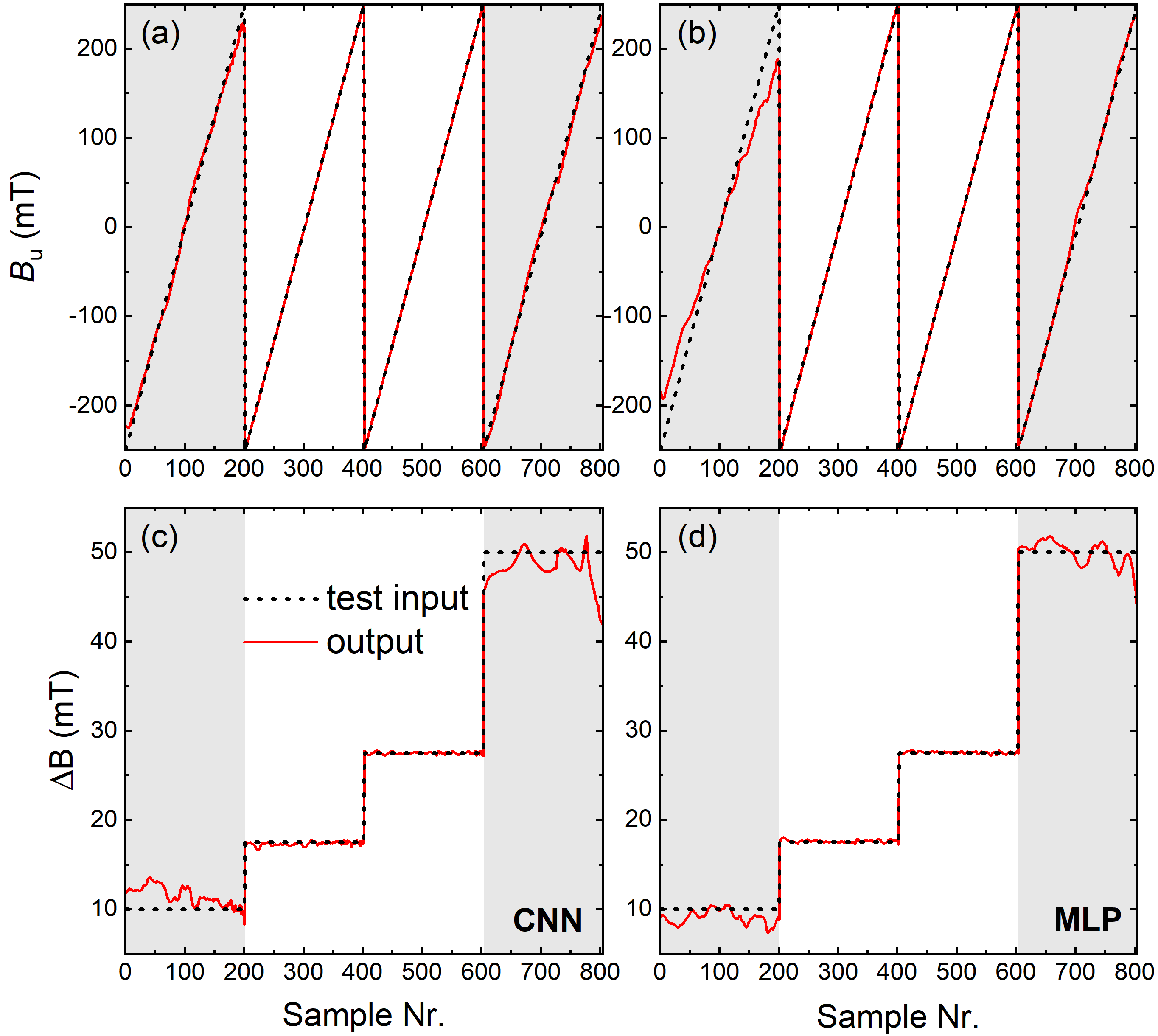
Once the training of the NN is complete, the weights are fixed. An FMR spectrum that is introduced to the NN will undergo the transformations based on the individual architecture and the NN will produce a prediction for the parameters and . Both NN were tested with unseen FMR spectra, i.e., 804 spectra outside of the training data generated with the same 201 values for and four values for (10, 17.5, 27.5 and 50 mT). Part of the test data fell within the range of the training set ( mT and mT) and part of it was beyond the training set ( mT and mT). In Fig. 5, the shaded regions correspond to data that lies outside of the training range, and while the agreement between prediction and target is not as good as for the data that was within the training range, it is remarkable that both NN were able to come close to the truth and predict material parameters that were in reasonable agreement to the real values.

In comparing the two NN, both performed exceptionally well for the data that was within the training range, whereas for data outside the training range, the CNN performed better in predicting and the MLP performed better in predicting . The performance of both NN can be assessed from the agreement between predicted and target values for both and , which we quantified with the Mean Absolute Error (MAE), shown in Table 1. The MAE for the training and the test with in-range data is comparable for both NN and it is on average smaller than 0.5 mT. For out-of-range data, the MAE is larger but still on the order of a few mT. This suggests that a properly trained NN can identify the correct material parameters from an FMR spectrum with relatively high accuracy.
| MAE (mT) | Training | Test in range | Test out of range |
|---|---|---|---|
| CNN | |||
| MLP | |||
| MAE (mT) | Training | Test in-range | Test out of range |
| CNN | |||
| MLP |
Figure 6 shows selected examples of FMR spectra from the test set, which were outside the training range versus the associated predicted FMR spectra computed using parameters predicted by the NN. It appears that for smaller linewidth the deviations are larger than for broader spectra. Despite this and the fact that the MAE is larger for out-of-range data, it is remarkable that both NN were able to predict reasonable and outside their training range. Considering the simple model we investigated here, with only two parameters, is a material parameter and does not depend on the measurement technique, thus CNN appears to be a better option for analyzing FMR spectra because it exhibits better performance in predicting .
Given the above, the use of neural networks for the spectral regression in order to obtain the material parameters is quite promising and further investigations are needed to fully harvest the potential of these techniques. Important future steps are to investigate FMR spectra with more parameters, i.e., to introduce additional anisotropy fields typically present in real materials, such as cubic anisotropy fields or surface anisotropy fields. Additionally, these techniques could be enhanced by tailoring the loss function to the particular problem, in what is termed as physics-informed machine learning.
V Conclusions
We have shown here that artificial neural networks, specifically with the examples of a convolutional neural network and a multi-layer perceptron, inverse problems of ferromagnetic resonance can be solved by training the network with pre-computed FMR spectra and creating associations between material parameters and spectrum structure. Both architectures were able to successfully predict the correct material parameters by identifying the FMR spectra with an absolute mean error smaller than 1 mT. Strikingly, the networks were able to predict material parameters that were not part of the training set with a reasonable agreement to the real values, showing potential for extrapolation within a reasonable parameter range. These results highlight the potential of using neural networks in spectroscopic data analysis for the identification of material properties, and with further optimization of the architecture and training protocols, these techniques can be used for high-throughput spectroscopic analyses of magnetic nanoparticles for a wide range of applications.
ACKNOWLEDGMENTS
MC is grateful for funding by the Louisiana Board of Regents [Contract No. LEQSF(2020-23)-RD-A-32]. Portions of this research were conducted with high performance computational resources provided by the Louisiana Optical Network Infrastructure (http://www.loni.org).
Data Availability
The data that support the findings of this study are available from the corresponding author upon reasonable request.
References
- Pankhurst et al. (2003) Q. A. Pankhurst, J. Connolly, S. K. Jones, and J. Dobson, J. Phys. D: Appl. Phys. 36, R167 (2003).
- McBain et al. (2008) S. McBain, H. H. P. Yiu, and J. Dobson, Int. J. Nanomed. 3, 169 (2008).
- Colombo et al. (2012) M. Colombo, S. Carregal-Romero, M. F. Casula, L. Gutiérrez, M. P. Morales, I. B. Böhm, J. T. Heverhagen, D. Prosperi, and W. J. Parak, Chem. Soc. Rev. 41, 4306 (2012).
- Dürr et al. (2013) S. Dürr, C. Janko, S. Lyer, P. Tripal, M. Schwartz, J. Zaloga, R. Tietze, and C. Alexiou, Nanotechnol. Rev. 2, 395 (2013).
- Périgo et al. (2015) E. A. Périgo, G. Hemery, O. Sandre, D. Ortega, E. Garaio, F. Plazaola, and F. J. Teran, Appl. Phys. Rev. 2, 041302 (2015).
- Ruta et al. (2015) S. Ruta, R. Chantrell, and O. Hovorka, Sci. Rep. 5, 9090 (2015).
- Chandrasekharan et al. (2018) P. Chandrasekharan, Z. W. Tay, X. Y. Zhou, E. Yu, R. Orendorff, D. Hensley, Q. Huynh, K. L. B. Fung, C. C. VanHook, P. Goodwill, B. Zheng, and S. Conolly, Br. J. Radiol. 91, 20180326 (2018).
- Materón et al. (2021) E. M. Materón, C. M. Miyazaki, O. Carr, N. Joshi, P. H. Picciani, C. J. Dalmaschio, F. Davis, and F. M. Shimizu, Appl. Surf. Sci. Adv. 6, 100163 (2021).
- Weiss et al. (2004) B. P. Weiss, S. S. Kim, J. L. Kirschvink, R. E. Kopp, M. Sankaran, A. Kobayashi, and A. Komeili, Earth Planet. Sci. Lett. 224, 73 (2004).
- Gehring et al. (2011) A. U. Gehring, J. Kind, M. Charilaou, and I. García-Rubio, Earth Planet. Sci. Lett. 309, 113 (2011).
- Blattmann et al. (2020) T. M. Blattmann, B. Lesniak, I. García-Rubio, M. Charilaou, M. Wessels, T. I. Eglinton, and A. U. Gehring, Earth Planet. Sci. Lett. 545, 116400 (2020).
- Myrovali et al. (2016) E. Myrovali, N. Maniotis, A. Makridis, A. Terzopoulou, V. Ntomprougkidis, K. Simeonidis, D. Sakellari, O. Kalogirou, T. Samaras, R. Salikhov, M. Spasova, M. Farle, U. Wiedwald, and M. Angelakeris, Sci. Rep. 6, 37934 (2016).
- Moreno et al. (2020) R. Moreno, S. Poyser, D. Meilak, A. Meo, S. Jenkins, V. K. Lazarov, G. Vallejo-Fernandez, S. Majetich, and R. F. L. Evans, Sci. Rep. 10, 2722 (2020).
- Slay et al. (2021) D. Slay, D. Cao, E. C. Ferré, and M. Charilaou, J. Appl. Phys. 130, 113902 (2021), https://doi.org/10.1063/5.0060769 .
- Kittel (1948) C. Kittel, Phys. Rev. 73, 155 (1948).
- Shapiro (1966) H. M. Shapiro, in International Series of Monographs in Solid State Physics, edited by S. V. Vonsovskii (Pergamon Press, Oxford, 1966).
- von Bardeleben et al. (2020) H. J. von Bardeleben, J. L. Cantin, and F. Gendron, “Ferromagnetic resonance spectroscopy: Basics and applications,” in Electron Paramagnetic Resonance Spectroscopy: Applications (Springer International Publishing, Cham, 2020) pp. 351–383.
- de Biasi and Devezas (1978) R. S. de Biasi and T. C. Devezas, J. Appl. Phys. 49, 2466 (1978).
- Kliava and Berger (1999) J. Kliava and R. Berger, J. Magn. Magn. Mater. 205, 328 (1999).
- Berger et al. (2000) R. Berger, J. Kliava, J.-C. Bissey, and V. Baietto, J. Appl. Phys. 87, 7389 (2000).
- Berger et al. (2001) R. Berger, J.-C. Bissey, J. Kliava, H. Daubric, and C. Estournés, J. Magn. Magn. Mater. 234, 535 (2001).
- Sukhov et al. (2008) A. Sukhov, K. Usadel, and U. Nowak, J. Magn. Magn. Mater. 320, 31 (2008).
- de Biasi et al. (2003) E. de Biasi, C. Ramos, and R. Zysler, J. Magn. Magn. Mater. 262, 235 (2003).
- de Biasi et al. (2013) E. de Biasi, E. Lima, C. Ramos, A. Butera, and R. Zysler, J. Magn. Magn. Mater. 326, 138 (2013).
- Raikher and Stepanov (1994) Y. L. Raikher and V. I. Stepanov, Phys. Rev. B 50, 6250 (1994).
- Poperechny and Raikher (2016) I. S. Poperechny and Y. L. Raikher, Phys. Rev. B 93, 014441 (2016).
- Noginova et al. (2007) N. Noginova, F. Chen, T. Weaver, E. P. Giannelis, A. B. Bourlinos, and V. A. Atsarkin, J. Phys.: Condens. Matt. 19, 246208 (2007).
- Noginova et al. (2008) N. Noginova, T. Weaver, E. P. Giannelis, A. B. Bourlinos, V. A. Atsarkin, and V. V. Demidov, Phys. Rev. B 77, 014403 (2008).
- Gazeau et al. (1999) F. Gazeau, V. Shilov, J. C. Bacri, E. Dubuis, F. Gendron, R. Perzynski, Y. L. Raikher, and V. I. Stepanov, J. Magn. Magn. Mater. 202, 535 (1999).
- Schmool and Schmaltz (2000) D. S. Schmool and M. Schmaltz, J. Non-Cryst. Sol. 353, 738 (2000).
- Li et al. (2009) H. Li, M. T. Klem, K. B. Sebby, D. J. Singel, M. Young, T. Douglas, and Y. U. Idzerda, J. Magn. Magn. Mat. 321, 175 (2009).
- Usselman et al. (2012) R. J. Usselman, S. E. Russek, M. T. Klem, M. A. Allen, T. Douglas, M. Young, Y. U. Idzerda, and D. J. Singel, J. Appl. Phys. 112, 084701 (2012).
- Smit and Beljers (1955) J. Smit and H. G. Beljers, Philips Res. Rep. 10, 113 (1955).
- Suhl (1955) H. Suhl, Phys. Rev. 97, 555 (1955).
- Baselgia et al. (1988) L. Baselgia, M. Warden, F. Waldner, S. L. Hutton, J. E. Drumheller, Y. Q. He, P. E. Wigen, and M. Maryško, Phys. Rev. B 38, 2237 (1988).
- Usov and Serebryakova (2022) N. A. Usov and O. N. Serebryakova, Sci. Rep. 12, 3126 (2022).
- Rosenblatt (1962) F. Rosenblatt, Principles of Neurodynamics: Perceptrons and the theory of brain mechanics (Spartan Books, Washington D.C., 1962).
- LeCun et al. (2015) Y. LeCun, Y. Bengio, and G. Hilton, Nature 521, 436 (2015).
- Kovacs et al. (2019) A. Kovacs, J. Fischbacher, H. Oezelt, M. Gusenbauer, L. Exl, F. Bruckner, D. Suess, and T. Schrefl, J. Magn. Magn. Mater. 491, 165548 (2019).
- Makaveev et al. (2001) D. Makaveev, L. Dupré, M. D. Wulf, and J. Malkebeek, J. Appl. Phys. 89, 6737 (2001).
- Antonio et al. (2021) S. Q. Antonio, F. R. Fulginei, A. Laudani, A. Faba, and E. Cardelli, J. Magn. Magn. Mater. 528, 167735 (2021).
- Yekta et al. (2019) P. V. Yekta, F. J. Honar, and M. N. Fesharaki, Comp. Mater. Sci. 159, 349 (2019).
- Kovacs et al. (2022) A. Kovacs, L. Exl, A. Kornell, J. Fischbacher, M. Hovorka, M. Gusenbauer, L. Breth, H. Oezelt, D. Praetorius, D. Suess, and T. Schrefl, J. Magn. Magn. Mater. 548, 168951 (2022).
- Charilaou et al. (2011) M. Charilaou, M. Winklhofer, and A. U. Gehring, J. Appl. Phys. 109, 093903 (2011).
- Charilaou (2017) M. Charilaou, J. Appl. Phys. 122, 063903 (2017).
- Guimarães (2009) A. P. Guimarães, Principles of Nanomagnetism (Springer, 2009).
- Morrish (2001) A. H. Morrish, The Physical Principles of Magnetism (Wiley-IEEE Press New York, 2001).
- Bickford (1950) L. R. Bickford, Phys. Rev. 78, 449 (1950).
- Gilbert (2004) T. Gilbert, IEEE Trans. Magn. 40, 3443 (2004).
- Hickey and Moodera (2009) M. C. Hickey and J. S. Moodera, Phys. Rev. Lett. 102, 137601 (2009).
- Kingma and Ba (2015) D. P. Kingma and J. Ba, in 3rd International Conference on Learning Representations, ICLR 2015, San Diego, CA, USA, May 7-9, 2015, Conference Track Proceedings, edited by Y. Bengio and Y. LeCun (2015).
- Abadi et al. (2015) M. Abadi, A. Agarwal, P. Barham, E. Brevdo, Z. Chen, C. Citro, G. S. Corrado, A. Davis, J. Dean, M. Devin, S. Ghemawat, I. Goodfellow, A. Harp, G. Irving, M. Isard, Y. Jia, R. Jozefowicz, L. Kaiser, M. Kudlur, J. Levenberg, D. Mané, R. Monga, S. Moore, D. Murray, C. Olah, M. Schuster, J. Shlens, B. Steiner, I. Sutskever, K. Talwar, P. Tucker, V. Vanhoucke, V. Vasudevan, F. Viégas, O. Vinyals, P. Warden, M. Wattenberg, M. Wicke, Y. Yu, and X. Zheng, “TensorFlow: Large-scale machine learning on heterogeneous systems,” (2015), software available from tensorflow.org.
- Moshagen et al. (2021) T. Moshagen, N. A. Adde, and A. N. Rajgopal, arXiv:2101.10426 (2021), 10.48550/ARXIV.2101.10427.