Supplemental material
The hybrid approach – Convolutional Neural Networks and Expectation Maximization Algorithm – for Tomographic Reconstruction of Hyperspectral Images

This supplemental material accompanies the main paper and details the computed tomography imaging spectrometer (CTIS) simulator as well as the measurement of the parameters used in the simulator. Additionally, RGB visualizations of all the hyperspectral images captured with our VIS-NIR laboratory pushbroom system are shown. A selection of the reconstructed hyperspectral images for both the 25- and 100-channel cases are also compared through RGB visualizations.

The CTIS simulator introduced in our work is an updated version of the simulator used in our previous work ¹, and is used to create input CTIS images for our network. This updated simulator includes zero mean white Gaussian noise, a point spread function (PSF) and spectral sensitivity corrections due to the illuminant and the diffractive optic element (DOE). Thus, the simulator requires the following inputs; x, y, z, b1, b2, shift, allOrders, diff_sens, illum, sigma_psf and noise. The first seven inputs determine the geometry of simulated CTIS image while the latter three inputs determine the optical parameters.

Figure S1a shows an overview of how the geometric inputs correlate to the simulated CTIS image: x, y, and z denote the two spatial and one spectral dimension of the input respectively, i.e. the zeroth order size is defined by x$\times$y and z denotes the number of spectral channels. b1 and b2 determine the number of pixels between the zeroth- and first orders and the first orders and the outer border of the image, respectively. b2 is usually set to zero, but provided for generalizability. The shift input determines the pixel-shift between consecutive spectral channels in the first order diffraction spots. It should be mentioned, that the user is responsible for setting the inputs to the correct values to match the true CTIS system, i.e. b1, b2 and shift are not calculated in the simulator based on the wavelengths of the spectral channels. The allOrders input is a boolean parameter, which simulates all eight surrounding first order diffraction spots if set to true and only the four (no skew orders) first order diffraction spots if set to false.

The optical parameters of the CTIS system is defined by the diff_sens, the illum and the applied noise. Additionally, the point-spread-function (PSF), sigma_psf, is set within the simulator, but is not available to the user as an input. The measurement of the PSF for the true CTIS system is detailed in Section S3. The diff_sens describes the wavelength- and diffraction order dependent sensitivity and must be a matrix of dimensions $\#\text{ orders}\times$z, i.e. in the case of allOrders = true, $9\times$z. The acquisition of the diffraction sensitivity is described in Section S4. The illuminant used in the simulator is a standard halogen-tungsten lamp, which is used for the acquisition of true CTIS images. The illumination input is a vector of size $1\times z$, which contains the spectrum of the illuminant measured with an intensity calibrated Avaspec 2048x14 spectrometer operating in the 200-720 nm range. The spectrometer was calibrated using a radiometrically calibrated light source (HL-3P-CAL) from Ocean Insights.

Figure S1b shows a simulated $450\times 450$ pixels CTIS image of a $100\times 100\times 25$ white cube, i.e. all voxels are set to 1, with b1 = 27, b2 = 0, shift = 2, allOrders = true, sigma_psf = $\sigma=1.04$ pixels and noise = 0.44. The diffraction sensitivity and illumination is set to the values defined in Section S4.

The PSF of the CTIS system is determined using the slanted-edge method ², where a sharp, slanted image is imaged and the PSF is estimated from the transition of the edge. In practice, a back illuminated razorblade is imaged by the CTIS camera (Figure S2a), and the edge spread function (ESF) (Figure S2c) is calculated as the mean profile across 250 pixels (blue rectangle) over the transition in the zeroth order (Figure S2b). The line spread function (LSF) is depicted in Figure S2d, and it is calculated as the derivative of the ESF, which is equivalent to a 2D slice of the PSF. Thus, assuming a spatially symmetric PSF, the LSF is an approximate estimate of the PSF. The standard deviation of the LSF (and PSF) is determined to be 1.04 pixels based on a Gaussian fit with $R^{2}=0.98$. The effect of the PSF on a single pixel is visualized in Figure S2e for a standard deviation of 1.04, which is the value used in the simulator.

The diffraction sensitivity of the CTIS system is measured using a monochromator (Newport mini, model: 78027) equipped with a halogen lamp (Tungsten Halogen Light Source, model: 78043), which is calibrated with an intensity calibrated Avaspec 2048x14 spectrometer. The spectrometer is calibrated using a radiometrically calibrated light source (HL-3P-CAL) from Ocean Insights. Since the measurements are conducted with the whole CTIS system, both the diffraction efficiency of the DOE, the transmission of the optical system, the CMOS image sensor response and optical aberrations are intrinsically a part of the acquired images. Thus, the measured diffraction sensitivity estimates the combined contribution from all these contributions. The monochromator output is centered in the zeroth order of the CTIS image, and CTIS images and corresponding dark-frame images are captured for wavelengths ranging from 400-750 nm with 25 nm steps. For each wavelength, the exposure time of the CTIS is set to maximize the dynamic range of the image sensor, and the dark frame is captured at the same exposure. Figure S1a shows the superimposed CTIS images of the monochromator for 400-750 nm.

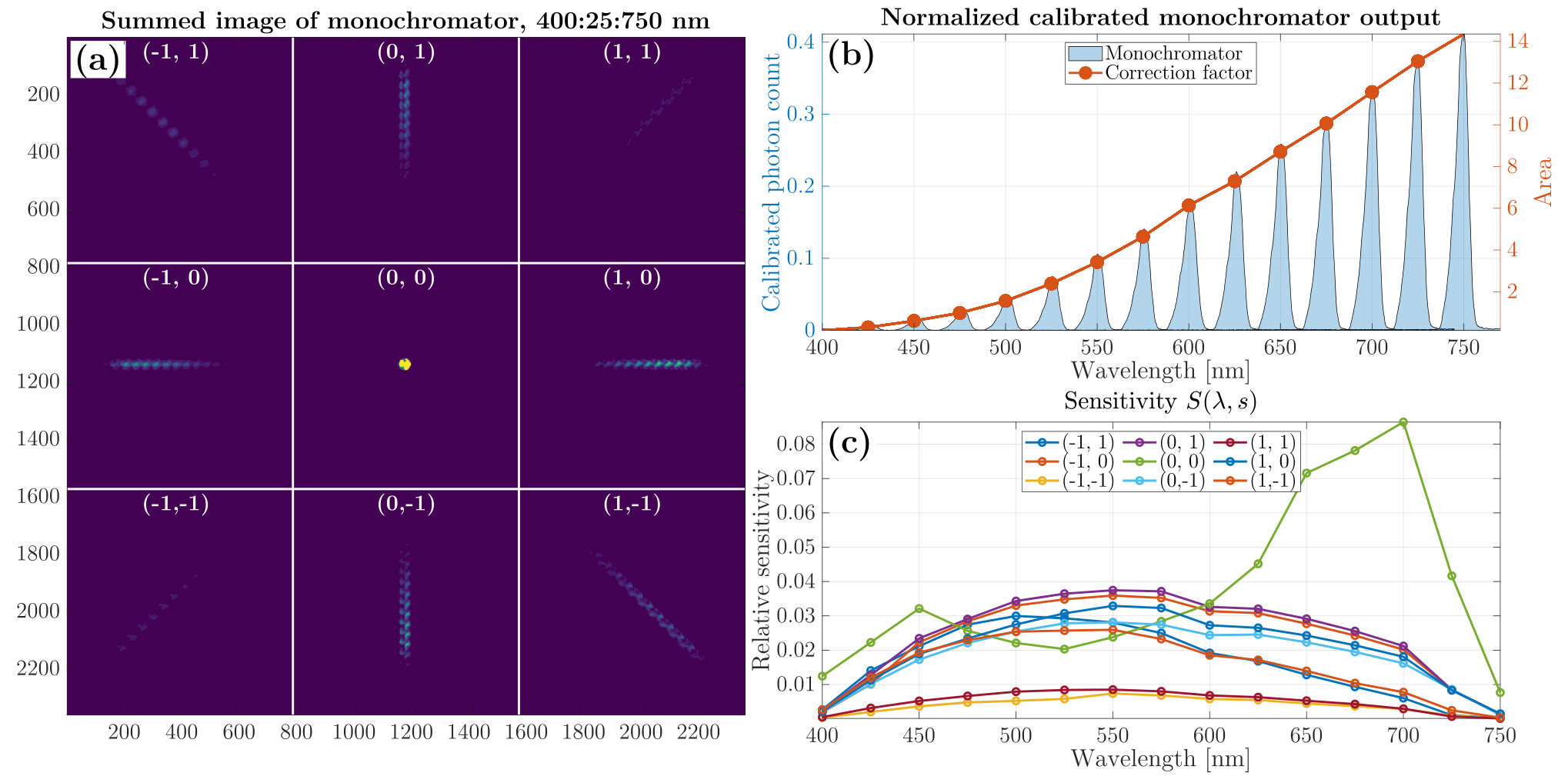
To determine the diffraction sensitivity $S(\lambda,s)$ from the acquired images, the dark frame is subtracted from the CTIS image, and the total photon count $PC(\lambda,s)$ for each diffraction spot (zeroth- and surrounding first orders) is divided with the product of the exposure time $t(\lambda)$ in µs, the camera gain $G(\lambda)$ (set to 1 for all images) and the wavelength correction factor $C(\lambda)$ from the spectrometer:

where $\lambda$ and $s$ denote the wavelength in nm and $s$ the diffraction spot, respectively. The monochromator output (Figure S1b) is used to determine the correction factors $C(\lambda)$, which indicate the relative intensity of the monochromator output (area in blue under the curve). The total photon count of the respective diffraction spots $PC(\lambda,s)$ is determined from the acquired CTIS images as the total volume of each spot. Figure S1c shows the calculated diffraction sensitivity $S(\lambda,s)$, where the indices ($i$, $j$) of the diffraction spots indicate (rows, columns). The DOE is designed to achieve a symmetric diffraction efficiency in the first orders while minimizing the zeroth order. The diffraction sensitivity of the zeroth order (0,0) is smallest for the lower wavelengths before increasing towards 700 nm, while the first order diffraction sensitivities all follow the same parabolic shape. However, the right-diagonal first orders {(-1,1) and (1,1)} have significantly lower diffraction sensitivity across the entire wavelength range. It should be noted, that since $S(\lambda,s)$ is only measured for 15 different wavelengths from 400-750 nm, the sensitivities are interpolated for the 25 and 100 channels used in this work.

The intensity calibrated Avaspec 2048x14 spectrometer is used to measure the output of an industrial halogen lamp used as illumination for the acquisition of CTIS images. Figure S1 shows the measured spectrum of the halogen lamp and a fitted black body with a temperature of $T=2952$ K°, which is consistent with standard $T=3000$ K° halogen lamps .

Figure S1-S4 shows RGB reconstructions of the 178 hyperspectral images captured with the VIS-NIR pushbroom system, which were used to generate data sets of CTIS images for the networks. The RGB images are generated by combining three spectral channels at 470 nm (blue), 549 nm (green) and 650 nm (red).

Figure S1-S3 show comparisons of the ground truth (GT) RGB visualization with the reconstructed RGB images for EM(20 iterations), CNN, CNN-EM(10 iterations), EM(10 iterations)-CNN, UNet and UNet-EM(10 iterations) for various hyperspectral images. The RGB images are generated by combining the 7th, 9th and 13th channel. Figure S1 and S2 contain seen cubes used in the training, while Figure S3 contains unseen cubes.

Figure S1-S3 show comparisons of the ground truth (GT) RGB visualization with the reconstructed RGB images for EM(20 iterations), UNet and UNet-EM(10 iterations) for various hyperspectral images. The RGB images are generated by combining the 14th, 29th and 48th channel. Figure S1 and S2 contain seen cubes used in the training, while Figure S3 contains unseen cubes.

References

- Huang et al. 2022 W.-C. Huang, M. S. Peters, M. J. Ahlebaek, M. T. Frandsen, R. L. Eriksen, and B. Jørgensen, Displays , 102218 (2022).
- Estribeau and Magnan 2004 M. Estribeau and P. Magnan, in Detectors and Associated Signal Processing, Vol. 5251, edited by J.-P. Chatard and P. N. J. Dennis (SPIE, 2004) pp. 243 – 252, backup Publisher: International Society for Optics and Photonics.