Calibration of nuclear charge density distribution by back-propagation neural networksPreprint: RIKEN-iTHEMS-Report-22
Abstract
Based on the back-propagation neural networks and density functional theory, a supervised learning is performed firstly to generate the nuclear charge density distributions. The charge density is further calibrated to the experimental charge radii by a composite loss function. It is found that, when the parity, pairing, and shell effects are taken into account, about of the nuclei in the validation set fall within two standard deviations of the predicted charge radii. The calibrated charge density is then mapped to the matter density, and further mapped to the binding energies according to the Hohenberg-Kohn theorem. It provides an improved description of some nuclei in both binding energies and charge radii. Moreover, the anomalous overbinding in 48Ca implies the existence of an indispensable beyond-mean-field effect.
Introduction—The charge density distribution, experimentally given by electron scattering experiments Angeli and Marinova 2013; Helm 1956; Hofstadter 1956, is essential for extracting nuclear structure information, including the shell-structure evolution, shape coexistence, shape transition, and neutron-skin thickness Campbell et al. 2016; Wood et al. 1992; Bender et al. 2003; Li et al. 2016. The relative radii of neighboring nuclei can also be determined using muonic-atom spectra as well as isotope shifts of laser spectroscopy Angeli and Marinova 2013. Since a strong connection exists between charge densities and matter densities, one generally calculates the charge density distribution by merging the nucleon form factors Dreher et al. 1974; Friar and Negele 1975 with the matter densities determined by scattering experiments, the () reaction Mutschler et al. 2016, or even heavy-ion collisions Fan et al. 2019.
Early on, the Fermi distributions Yennie et al. 1954; Ullah 1994 and Fourier-Bessel expansion Euteneuer et al. 1978; Ullah 1994 were used to describe nuclear matter and charge densities approximately. With the development of computational power, various branching models Bardeen et al. 1957; Bogoljubov et al. 1958; Dytrych et al. 2007; Dean et al. 2008; Roth 2009; Dytrych et al. 2013; Neff et al. 2015; Zhang et al. 2017; Naito et al. 2019; Bertulani and Valencia 2019 derived from density functional theory (DFT) and shell model calculation have become more popular among theorists. However, due to the complexity of nuclear many-body systems, the calculations of these theories still face challenges in describing the beyond-mean-field effects and nucleon-nucleon correlations Yang et al. 2019; Tanaka et al. 2021; Duer et al. 2018; Miller 2019.
For nuclear complex systems, back-propagation neural networks Rumelhart et al. 1986 have achieved a series of success in various aspects, such as nuclear masses Niu and Liang 2018; Ma et al. 2020; Athanassopoulos et al. 2004, nuclear spins and parities Gernoth et al. 1993, charge radii Utama et al. 2016a; Wu et al. 2020; Dong et al. 2022; Co' et al. 2022, excited states Lasseri et al. 2020; Wang et al. 2022, extrapolation problems in an method Negoita et al. 2019, -decay half-lives Saxena et al. 2021, -decay half-lives Niu et al. 2019, fission yields Wang et al. 2019; Qiao et al. 2021, and so on. Most present neural networks learn and predict the residuals between theoretical and experimental values, which has an advantage that the corrected predictions are more accurate than the existing theoretical model Niu and Liang 2018; Utama et al. 2016b; Niu et al. 2019. However, the corrections have weak physical interpretability and it is difficult to predict different observables consistently. Google proposed a hybrid quantum-classical machine learning model for training beyond classical data types, where back-propagation is used to tune the quantum logic gate parameters, allowing for deep integration of physics and neural networks Broughton et al. 2020.
Based on the Hohenberg-Kohn maps Moreno et al. 2020 of DFT and the proven strong generalization ability of neural networks in describing density distributions Yang et al. 2021, in this letter, we collectively constrain the charge density distributions by back-propagation with experimental data of charge radii, which makes the residual information flow back from radii to densities. We also construct the map from charge density to binding energy to achieve further transfer of information from radius to binding energy.
The charge density generators—Previously, a multilayer feed-forward neural network with a back-propagation algorithm of error has been elaborated to perform the maximum likelihood estimation in the process of generating density distributions Yang et al. 2021 approximating the theoretical calculation. It is shown that a network trained by the density distributions of about 200–300 nuclei is sufficient to describe the density distributions of all the nuclei on the nuclear chart and has a powerful extrapolation capability Yang et al. 2021.
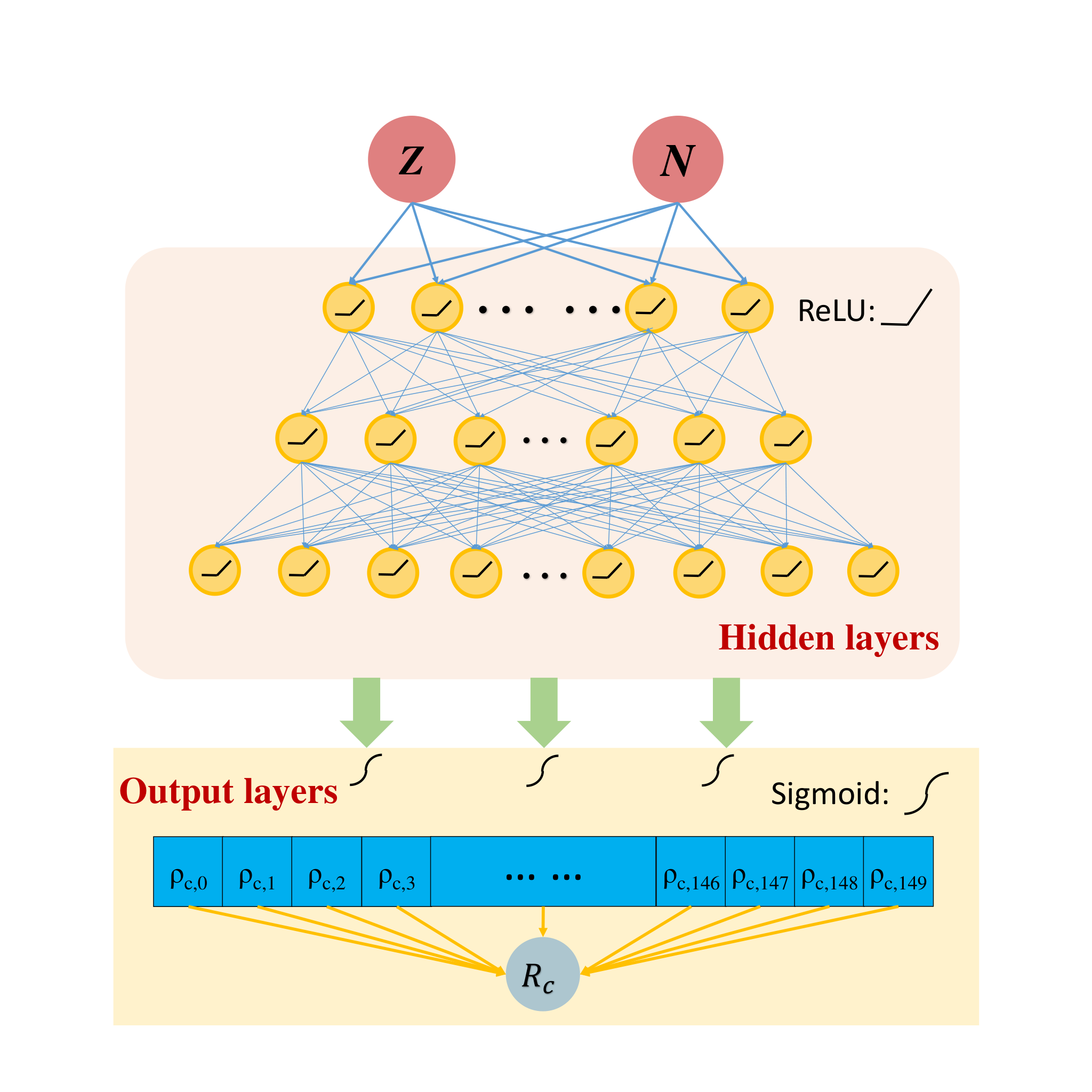
Based on such a high computational efficiency and generalization ability, in this study we introduce the correlation between the theoretical charge density and the experimental root-mean-square charge radius () to a new hybrid neural network. The structure of this network is shown in Fig. 1, where is the density on the mesh with (). The input is the proton and neutron numbers of a nuclide, . The outputs are the charge density and root-mean-square charge radius gained by the customized integration layer ,
| (1) |
where is the normalized predicted charge density distribution, i.e., . For the hidden module, three attempts are made: 1. A deep fully connected neural network; 2. A convolutional neural network, suitable for learning the gradient information of features; 3. A neural network with a feature layer , containing the parity, paring, and shell effects,
| (2) |
where
| (3) | ||||||
and () is the difference between the actual nucleon number () and the nearest magic number (8, 20, 28, 50, 82, or 126). Hereafter, we refer to the three schemes of neural networks as charge density generator-1 (CDG-1), CDG-2, and CDG-3, respectively. See Supplemental Materials (SM) for details. The map is denoted as
| (4) |
where is the set of trainable parameters.
In general, the charge density distribution calculated by physical models , e.g., that calculated by the Skyrme Hartree-Fock (SHF) theory with the Bardeen-Cooper-Schrieffer (BCS) pairing, is expected to be quite accurate. The residuals between theory and experiment can be eliminated by assuming a correction to the charge density , satisfying . We refer this process as calibration. The calibrated charge density distribution , whose is expected to be close to Angeli and Marinova 2013, can be obtained by
| (5) |
Additionally, we aim at making the smallest possible corrections to the theory.
To this end, we design a composite loss function. The normalized mean-square-error Yang et al. 2021 is employed as an assessment of density distribution:
| (6) |
where indicates the number of grid points and the factor makes dimensionless. The charge density distributions are calculated by the SHF+BCS theory with the SkM* interaction Bartel et al. 1982. They are obtained from the charge form factor by the inverse Fourier-Bessel transform,
| (7) |
where is the spherical Bessel function. The contributions of matter density and spin-orbit current are folded in Reinhard 1991 (see SM for details). has a large range of variation (about –) and therefore the Pearson divergence is picked, i.e., its loss function reads
| (8) |
where the factor also makes dimensionless. The two loss functions and are combined as
| (9) |
where is the weighting factor and is batch size, which means that 64 nuclei are constrained simultaneously for each training session. Actually, the corrections for different nuclei are derived from the same parameter updates , i.e., the correction of each nucleus is uniformly constrained by the other nuclei. We randomly take 640 nuclei (10 batches) of about 900 nuclei measured to date as the training set. The remaining nuclei are recorded as the validation set (see SM for details). It is recorded as an epoch when all nuclei on the training set have been trained once.
Machine learning processes—The process of machine learning is divided into two stages: simulating the SHF+BCS results and correcting with experimental data. The evaluation of these processes is shown in Fig. 2. The first 3000 epochs are the stage of simulating the SHF+BCS results, during which is being minimized. One can see that the loss functions of the training and validation sets almost overlap. It means neither nor is overfitted, which shows the generalization ability of the network. The dashed magenta line is the Pearson divergence on the validation set between the SHF+BCS and experimental values:
| (10) |
where is the number of nuclei on the validation set. After a short training, the loss values overlap with . This indicates that the network naturally captures the information well in the process of learning the density distribution.
After 3000 epochs, the pre-trained model is further tuned with an objective function , which allows the importance of experimental data to slightly exceed that of theoretical calculations. Thus, the charge density distributions under constraints are spontaneously corrected by the network. Since the correction makes the predicted charge radius close to the experimental value and the distribution naturally deviate from the model, the value of falls and the value of jumps as shown in Fig. 2. It is clear that machine learning successfully eliminated a portion of residuals between SHF+BCS and experimental values. Such a process can be migrated to any other theoretical model. Remarkably, the training costs only 10 GPU minutes.
Calibrated charge density and charge radius—To explore the network performance, the errors of the densities and radii given by the CDG-1, CDG-2, and CDG-3 on the validation set are plotted in the inserts of Fig. 2. It can be seen that the errors by CDG-3 are minimal for both density and radius. This indicates the predictions of CDG-3 are closest to the experimental radii, while its corrections to the theory are smallest. This agrees with our assumption. Compared to CDG-1 and CDG-2, CDG-3 takes into account the odd-even staggering, pairing, and shell effects. Therefore, we conclude that the network structures considering more physical properties are more sufficient to improve the prediction accuracy, which is consistent with the mass research Niu and Liang 2018.

Accuracy is more intuitive to show the CDGs’ performance than error. Figure 3(a) shows the prediction accuracy of the three networks, where the accuracy indicates the percentages of the experimental data on the validation set falling within different predicted standard deviations (red for 1 , blue for 1.5 , and pink for 2 ). The values of accuracy are consistent with the errors on validation set shown in Fig. 2 for different networks, i.e., the smaller the error, the higher the accuracy. In particular, the numbers of experimental data falling within 2 standard deviations do not exceed for CDG-1 and CDG-2. Meanwhile, the accuracy of CDG-3 (1 ) is already close to , which even reaches for 2 . It can be speculated that CDG-3 can predict the radii of the remaining unmeasured nuclei with high precision. We present the predictions for nuclear charge radii in Fig. 3(b).

By taking several isotopic chains as examples, we compare the charge radii calculated by SHF+BCS and the predictions of CDG-3 with 1- error with the available experimental data in Fig. 4. It is found that CDG-3, containing the parity, paring, and shell effects, describes well the odd-even staggering for the Ca isotopes. Meanwhile, CDG-1 and CDG-2 failed in benchmarking the experimental data (see SM). For Pb isotopes, CDG-3 performs comparably with the theoretical model. The present predictions almost match the experimental data in the case of training several Pb isotopes. In particular, the predictive power remains strong even when we remove the Ca and Pb isotopes from the training set (see SM). Given the excellent performance of CDG-3, we predicted the untrained Dy and Tb isotopes. For the Dy isotopes, the predictions are in agreement with experiment, but with much smaller uncertainty than the experimental error. For the Tb isotopes, compared to the SHF+BCS results, the predicted isotope shifts are in good agreement with the experimental data, although the predicted charge radii are systematically larger than the present experimental central values by fm. The above predictions can be testified in the coming experiments.
Map from charge density to binding energy—According to the Hohenberg-Kohn theorem Hohenberg and Kohn 1964; Moreno et al. 2020, there exists a bijective map between the local matter density and the one-body potential. This means that the corrections on the density distributions can be mapped to other observables, such as binding energies Ryczko et al. 2019. Thus, we reconstruct a map from charge density to binding energy (CDTBE). The schematic structure of such a feedforward neural network is shown in Fig. 5. There are three parts in the CDTBE map—M1, M2, and M3. M1 is the previously trained charge density generator, and we take the CDG-3; M2 is a map from charge density to matter density as the inverse of Eq. (7); M3 is a map from the neutron, proton, and charge densities to the binding energy per nucleon. M2 and M3 are trained by the densities and binding energies of SHF+BCS with effective interactions SkM, SkM*, SkIII, SLy4, SkT, and SkT3 Friedrich and Reinhard 1986 (See SM for details). It is found that the networks adequately captures the relationship between densities and binding energy with different DFT effective interactions. As the charge density updates in CDG-3, the residual information flows to other observables, i.e., .
Taking the Ca isotopes as examples, the binding energies per nucleon obtained by the CDG-3 residual information flow are shown in Fig. 6. We note that the propagated corrections provide a better description, except 47,48,49Ca. Especially for 40,42,44Ca, both radii (see Fig. 4(a)) and binding energies coincide well with the experimental values. This illustrates that the physical features contained in the CDTBE map based on density functional theory are adequate for these nuclei. In contrast, for 48Ca, the radius is corrected to a smaller value than that of SHF+BCS, leading to an increase of nuclear densities in the central region and a further decrease of binding energy, which is consistent with equation of state. However, it results in further deviations from the experimental value, which implies an indispensable beyond-mean-field effect near 48Ca, as discussed in Ref. Perera et al. 2021.
Summary—In this study, a novel supervised learning on the combination of the theoretical charge density distributions and the experimental charge radii has been performed. In such a way, the physics features embedded in nuclear density functional theory can be preserved to a large extent and the feedback from the experimental data can be considered quantitatively. It is found that the description of charge radii can be improved globally on the nuclear chart. In particular, the specific charge radii evolution in the Ca isotopes can be well reproduced by taking the parity, pairing, and shell effects into account. This property remains valid even when all the Ca isotopes are excluded in the learning set. The predictive power is also shown with the charge radii in the Dy and Tb isotopes, where the present experimental uncertainties are much larger than the prediction uncertainties.
Inspired by the Hohenberg-Kohn theorem, an information flow from charge density to binding energy has also been constructed and investigated. It is found that for the Ca isotopes the improvement in the description of charge radii can also be propagated to the improvement in the description of binding energies, except 47,48,49Ca. The corresponding analysis implies the existence of an indispensable beyond-mean-field effect near 48Ca.
Along this direction, we will not only improve the description of different nuclear observables consistently but also strengthen the interpretability of the supervised learning.
Acknowledgements.
Acknowledgements—This work is supported by the National Natural Science Foundation of China under Grants Nos. 12005175 and 11875070, the Fundamental Research Funds for the Central Universities under Grant No. SWU119076, the JSPS Grant-in-Aid for Early-Career Scientists under Grant No. 18K13549, the JSPS Grant-in-Aid for Scientific Research (S) under Grant No. 20H05648, and the Anhui project (Z010118169). This work is also partially supported by the RIKEN Pioneering Project: Evolution of Matter in the Universe, the RIKEN Special Postdoctoral Researchers Program, and the Science and Technology Hub Collaborative Research Program from RIKEN Cluster for Science, Technology and Inovation Hub (RCSTI).References
- Angeli and Marinova (2013) I. Angeli and K. Marinova, At. Data Nucl. Data Tables 99, 69 (2013).
- Helm (1956) R. H. Helm, Phys. Rev. 104, 1466 (1956).
- Hofstadter (1956) R. Hofstadter, Rev. Mod. Phys. 28, 214 (1956).
- Campbell et al. (2016) P. Campbell, I. Moore, and M. Pearson, Prog. Part. Nucl. Phys. 86, 127 (2016).
- Wood et al. (1992) J. Wood, K. Heyde, W. Nazarewicz, M. Huyse, and P. van Duppen, Phys. Rep. 215, 101 (1992).
- Bender et al. (2003) M. Bender, P.-H. Heenen, and P.-G. Reinhard, Rev. Mod. Phys. 75, 121 (2003).
- Li et al. (2016) X.-F. Li, D.-Q. Fang, and Y.-G. Ma, Nucl. Sci. Tech. 27 (2016), 10.1007/s41365-016-0064-z.
- Dreher et al. (1974) B. Dreher, J. Friedrich, K. Merle, H. Rothhaas, and G. Lührs, Nucl. Phys. A 235, 219 (1974).
- Friar and Negele (1975) J. Friar and J. Negele, Adv. Nucl. Phys. , 219 (1975).
- Mutschler et al. (2016) A. Mutschler, A. Lemasson, O. Sorlin, D. Bazin, C. Borcea, et al., Nat. Phys. 13, 152 (2016).
- Fan et al. (2019) X.-H. Fan, G.-C. Yong, and W. Zuo, Phys. Rev. C 99, 041601 (2019).
- Yennie et al. (1954) D. R. Yennie, D. G. Ravenhall, and R. N. Wilson, Phys. Rev. 95, 500 (1954).
- Ullah (1994) N. Ullah, Pramana 43, 165 (1994).
- Euteneuer et al. (1978) H. Euteneuer, J. Friedrich, and N. Voegler, Nucl. Phys. A 298, 452 (1978).
- Bardeen et al. (1957) J. Bardeen, L. N. Cooper, and J. R. Schrieffer, Phys. Rev. 106, 162 (1957).
- Bogoljubov et al. (1958) N. N. Bogoljubov, V. V. Tolmachov, and D. V. Širkov, Fortschr. Phys. 6, 605 (1958).
- Dytrych et al. (2007) T. Dytrych, K. D. Sviratcheva, C. Bahri, J. P. Draayer, and J. P. Vary, Phys. Rev. Lett. 98, 162503 (2007).
- Dean et al. (2008) D. J. Dean, G. Hagen, M. Hjorth-Jensen, T. Papenbrock, and A. Schwenk, Phys. Rev. Lett. 101, 119201 (2008).
- Roth (2009) R. Roth, Phys. Rev. C 79, 064324 (2009).
- Dytrych et al. (2013) T. Dytrych, K. D. Launey, J. P. Draayer, P. Maris, J. P. Vary, E. Saule, U. Catalyurek, M. Sosonkina, D. Langr, and M. A. Caprio, Phys. Rev. Lett. 111, 252501 (2013).
- Neff et al. (2015) T. Neff, H. Feldmeier, and W. Horiuchi, Phys. Rev. C 92, 024003 (2015).
- Zhang et al. (2017) Y. Zhang, Y. Chen, J. Meng, and P. Ring, Phys. Rev. C 95, 014316 (2017).
- Naito et al. (2019) T. Naito, X. Roca-Maza, G. Colò, and H. Liang, Phys. Rev. C 99, 024309 (2019).
- Bertulani and Valencia (2019) C. A. Bertulani and J. Valencia, Phys. Rev. C 100, 015802 (2019).
- Yang et al. (2019) Z. X. Yang, X. L. Shang, G. C. Yong, W. Zuo, and Y. Gao, Phys. Rev. C 100, 054325 (2019).
- Tanaka et al. (2021) J. Tanaka, Z. Yang, S. Typel, S. Adachi, S. Bai, et al., Science 371, 260 (2021).
- Duer et al. (2018) M. Duer et al. (CLAS), Nature 560, 617 (2018).
- Miller (2019) G. A. Miller, Phys. Rev. Lett. 123, 232003 (2019).
- Rumelhart et al. (1986) D. E. Rumelhart, G. E. Hinton, and R. J. Williams, Nature 323, 533 (1986).
- Niu and Liang (2018) Z. Niu and H. Liang, Phys. Lett. B 778, 48 (2018).
- Ma et al. (2020) C. Ma, M. Bao, Z. M. Niu, Y. M. Zhao, and A. Arima, Phys. Rev. C 101, 045204 (2020).
- Athanassopoulos et al. (2004) S. Athanassopoulos, E. Mavrommatis, K. Gernoth, and J. Clark, Nucl. Phys. A 743, 222 (2004).
- Gernoth et al. (1993) K. Gernoth, J. Clark, J. Prater, and H. Bohr, Phys. Lett. B 300, 1 (1993).
- Utama et al. (2016a) R. Utama, W.-C. Chen, and J. Piekarewicz, J. Phys. G: Nucl. Part. Phys. 43, 114002 (2016a).
- Wu et al. (2020) D. Wu, C. L. Bai, H. Sagawa, and H. Q. Zhang, Phys. Rev. C 102, 054323 (2020).
- Dong et al. (2022) X.-X. Dong, R. An, J.-X. Lu, and L.-S. Geng, Phys. Rev. C 105, 014308 (2022).
- Co' et al. (2022) G. Co', M. Anguiano, and A. M. Lallena, Phys. Rev. C 105, 034320 (2022).
- Lasseri et al. (2020) R.-D. Lasseri, D. Regnier, J.-P. Ebran, and A. Penon, Phys. Rev. Lett. 124, 162502 (2020).
- Wang et al. (2022) Y. Wang, X. Zhang, Z. Niu, and Z. Li, Phys. Lett. B 830, 137154 (2022).
- Negoita et al. (2019) G. A. Negoita, J. P. Vary, G. R. Luecke, P. Maris, A. M. Shirokov, et al., Phys. Rev. C 99, 054308 (2019).
- Saxena et al. (2021) G. Saxena, P. K. Sharma, and P. Saxena, J. Phys. G: Nucl. Part. Phys. 48, 055103 (2021).
- Niu et al. (2019) Z. M. Niu, H. Z. Liang, B. H. Sun, W. H. Long, and Y. F. Niu, Phys. Rev. C 99, 064307 (2019).
- Wang et al. (2019) Z.-A. Wang, J. Pei, Y. Liu, and Y. Qiang, Phys. Rev. Lett. 123, 122501 (2019).
- Qiao et al. (2021) C. Y. Qiao, J. C. Pei, Z. A. Wang, Y. Qiang, Y. J. Chen, N. C. Shu, and Z. G. Ge, Phys. Rev. C 103, 034621 (2021).
- Utama et al. (2016b) R. Utama, J. Piekarewicz, and H. B. Prosper, Phys. Rev. C 93, 014311 (2016b).
- Broughton et al. (2020) M. Broughton, G. Verdon, T. McCourt, A. J. Martinez, J. H. Yoo, et al. (2020) arXiv:2003.02989 .
- Moreno et al. (2020) J. R. Moreno, G. Carleo, and A. Georges, Phys. Rev. Lett. 125, 076402 (2020).
- Yang et al. (2021) Z.-X. Yang, X.-H. Fan, P. Yin, and W. Zuo, Phys. Lett. B 823, 136650 (2021).
- Bartel et al. (1982) J. Bartel, P. Quentin, M. Brack, C. Guet, and H.-B. Håkansson, Nucl. Phys. A 386, 79 (1982).
- Reinhard (1991) P.-G. Reinhard, in Computational Nuclear Physics 1 (Springer Berlin Heidelberg, 1991) pp. 28–50.
- Hohenberg and Kohn (1964) P. Hohenberg and W. Kohn, Phys. Rev. 136, B864 (1964).
- Ryczko et al. (2019) K. Ryczko, D. A. Strubbe, and I. Tamblyn, Phys. Rev. A 100, 022512 (2019).
- Friedrich and Reinhard (1986) J. Friedrich and P.-G. Reinhard, Phys. Rev. C 33, 335 (1986).
- Perera et al. (2021) U. C. Perera, A. V. Afanasjev, and P. Ring, Phys. Rev. C 104, 064313 (2021).