Scalable Distributional Robustness in a Class of Non Convex Optimization with Guarantees
Abstract
Distributionally robust optimization (DRO) has shown lot of promise in providing robustness in learning as well as sample based optimization problems. We endeavor to provide DRO solutions for a class of sum of fractionals, non-convex optimization which is used for decision making in prominent areas such as facility location and security games. In contrast to previous work, we find it more tractable to optimize the equivalent variance regularized form of DRO rather than the minimax form. We transform the variance regularized form to a mixed-integer second order cone program (MISOCP), which, while guaranteeing near global optimality, does not scale enough to solve problems with real world data-sets. We further propose two abstraction approaches based on clustering and stratified sampling to increase scalability, which we then use for real world data-sets. Importantly, we provide near global optimality guarantees for our approach and show experimentally that our solution quality is better than the locally optimal ones achieved by state-of-the-art gradient-based methods. We experimentally compare our different approaches and baselines, and reveal nuanced properties of a DRO solution.
1 Introduction
Distributionally robust optimization (DRO) is a popular approach employed in robust machine learning. Mostly, if not always, these works have focussed on the task of classification or regression. However, often in practical applications the end goal of learning is a decision output z, which requires yet another complex optimization that uses the output of a regressor . For example, in facility location problem the learning of facility values is followed by an optimization using the values predicted to decide where to locate facilities and in security games adversary behavior model is learned and then an optimal defense allocation computed based on the learned model. Often the learning output is provided as public datasets with no access to the underlying private dataset used for such learning. In this set-up, we aim to provide robustness at the decision making level with access to only the non-robust learning output .
However, often the objective of decision optimization is non-convex in the learning system output x unlike the convex objective of classification or regression, presenting significant scalability challenges. In general, for decision making and specifically for the problem domains we consider, global optimality is important as sub-optimal decisions can lead to large revenue loss or loss of life; thus, the local optimality provided by gradient based methods is not sufficient. As a consequence, in this paper, we study the scenario of calculating DRO decisions using the given multi-dimensional real valued outputs of a non-robust learned . A first result (Theorem 1) characterizes the quality of DRO decision output compared to the scenario where we know the true . Our main focus is on addressing the scalability issue for the DRO decision making problem for a particular, but widely used, class of sum of fractionals non-convex objective. This objective arises from the well-known discrete choice models Train 2003 of human behavior, which is known to not have scalable globally optimal solutions (Schaible 1995; Li et al. 2019); we use this for tackling two different decision optimization problem in facility location and a robust version of Bayesian Stackelberg security games problem with quantal response. As far as we know, this is a first attempt to solve the aforementioned non-convex problems in a DRO setting to near global optimality.
Our first contribution is a modelling construct, where we reformualate the variance regularized form Duchi and Namkoong 2019 of our non-convex sum of fractionals objective as a mixed integer second order cone program (MISOCP). While the MISOCP form provides more scalability than the original formulation and guaranteed solution quality (Theorem 2), it still does not scale to real world sized datasets. Our second contribution is a pair of approaches that achieves further scalability by splitting the problem space into sub-regions and solving a smaller MISOCP over representative samples from the sub-regions. Under mild conditions, both approaches provide global optimality guarantees (Theorem 3, 4).
Our final contribution is detailed experiments validating the scalability of our approaches on a simulated security game problem as well as two variants of location facility using park and ride data-sets from New York (Holguin-Veras et al. 2012). We compare with two gradient-based approaches (Lin et al. 2020) and show the superior solution quality achieved by our approach, which also reveals the need for global optimality. We further show a nuanced property of the DRO solution in providing better decisions for low probability scenarios over non-robust versions. Overall, our work provides desired robustness with globally optimal solution guarantees.
Related work: Our work is built on a recent line of research that connects the concepts of DRO and variance regularization (Duchi and Namkoong 2019; Duchi et al. 2021; Lam 2016; Maurer and Pontil 2009; Staib et al. 2019). While most the previous studies along this research line focus on convex and continuous problems or problems with submodular objectives, our work concerns a class of DRO problems with fractional structures, which are highly non-convex and requires new technical developments for globally optimal solution. Recent work Yan et al. 2020; Qi et al. 2021 has addressed non-convex objectives in DRO using gradient based methods that converge to stationary points, which is insufficient for decision making as we experimentally show that stationary points and globally optimal points can yield very different decision utilities.
The literature on DRO is vast and we refer the reader to Rahimian and Mehrotra 2019 for a review. DRO methods can be classified by different ways to define ambiguity sets of distributions, for instance, ambiguity sets based on -divergences (Ben-Tal et al. 2013; Duchi and Namkoong 2019; Staib et al. 2019) or Wasserstein distances (Pflug and Wozabal 2007; Esfahani and Kuhn 2018; Shafieezadeh-Abadeh et al. 2015; Blanchet and Murthy 2019). In this work, we focus on -divergence based models, motivated by their interesting connections with variance regularization and the tractability of the resulting non-convex DRO models.
We show that our DRO methods can be used in some popular decision-making problems such as Stackelberg security game (SSG) with Quantal Response (Tambe 2011; Xu 2016; Fang et al. 2017; Sinha et al. 2018; Yang et al. 2012; Haghtalab et al. 2016) or competitive facility location under random utilities (Benati and Hansen 2002; Freire et al. 2016; Mai and Lodi 2020; Dam et al. 2021). To the best of our knowledge, a DRO Bayesian model has not been studied in existing SSG works. In the context of competitive facility location under random utilities, we seem to be the first to bring DRO as a consideration. We handle a DRO version of a facility cost optimization problem, which has also never been studied in prior work.
2 Background, Preliminary Notation and Result
We use bold fonts for vectors and non-bold font for vector components and scalars, e.g., is a component of x. denotes . A -dimensional vector is written as or as . The positive part of a vector x is , and the negative part is . represent the all zero and all one vector.
Distributionally Robust Optimization: Consider a function with inputs being a decision variable z and parameter . Both z and x lie in an Euclidean space and both are constrained by linear constraints; for notational ease we skip writing the constraints in the general formulation. We seek to maximize the following objective function . For many classes of distributions the above is generally not tractable and one needs to sample x from . Let be samples, we can solve the sample average approximation (SAA) problem instead . Let be the empirical distribution induced by the samples. The SAA above is same as . A distributionally robust version of the SAA problem is , where the ambiguity set , and is the divergence: . The above optimization can be written equivalently as ( defined below)
| (DRO) |
where . We have earlier stated that is output by a regressor, say for some function class trained using loss with datapoints, but this implies that might not exactly same as for some underlying feature values and best function . We assume is deterministic and has zero Bayes risk. Let be the true distribution induced by from which the (unknown) samples ’s are obtained; hence, the true utility of a decision z is . We prove an end to end guarantee about the output decision using ’s, which reveals that is not much worse than the decision learned if would be available and used, and larger training data helps.
Theorem 1.
If the optimal decision when solving DRO is using ’s and using ’s, is -Lipschitz in x, is bounded, and a scaled upper bounds (i.e., for constants ) then, the following holds with probability : , where and is the Rademacher complexity with samples and are constants dependent on .
Variance Regularizer: As a large number of samples are needed for a low variance approximation of the true distribution, another proposed robust version of the SAA (Maurer and Pontil 2009; Duchi and Namkoong 2019) is to optimize the following variance-regularized (VR) objective function
| (VR) |
The above allows to directly optimize the trade-off between bias and variance. In a fundamental result, Duchi and Namkoong 2019 show that, with high probability, problem (VR) is equivalent to the problem (DRO). Further, Duchi and Namkoong 2019 argue for solving the DRO version of the problem for concave (note we are solving a maximization SAA problem) since concave results in concavity of , thus, the overall DRO problem is a concave maximization problem. In contrast, the objective in (VR) is not concave.
In this paper, our focus is on that is not concave, thus, the choice of DRO or variance regularized form is not obvious. For the class of functions that we analyze, we argue the variance regularized version is more promising as far as scalability for global optimality is concerned. We work with the assumption that the variance regularized form is equivalent to DRO, which holds under the mild condition shown in Equation (9) in Duchi and Namkoong 2019.
3 Towards a Globally Optimal Solution
In this section, we present results for a general class of non-concave functions that has a fractional form with non-linear numerator and denominator and that can be approximated by a linear fractional form with binary variables.
Then, we show three prominent applications of our approach.
Notation: For ease of notation, we use shorthand to denote by and by .
3.1 General Recipe to Form a MISOCP
We perform a sequence of variable and constraint transformations of (VR), leading to a MISOCP.
Mixed Integer Concave Program: The variance regularized objective in shorthand notation is:
| (1) |
We substitute and for all , such that and . The objective in Equation 1 thus becomes which is concave in the variables and . We add the new constraints and for all . Note that, while the objective is now concave with above changes, we have pushed the non-convexity into the constraints for all that are added to the optimization.
If can be written (or approximated) as a fraction with affine numerator and denominator, we can convert the constraint into a convex constraint, giving us an overall concave program. The conversion is explained next. Suppose can be written (or approximated) as where v represents binary variables after conversion (v completely replaces z and are dependent on ’s). Typically, such a linear fractional form is constructed via a piece wise linear approximation of the original non-linear numerator and denominator of . Assume v is of dimension ; typically will depend on the number of pieces. Define where . Then, we can (re)write the fractional form for as . This yields the linear constraints below with the non-linearity now restricted to . (2) (3) (4)
We handle using McCormick relaxation technique (McCormick 1976). Typically, McCormick relaxation is applied for bilinear terms that are the product of two continuous variables, in which case, it is an approximation. However, in our case since v is a binary vector variable, the McCormick relaxation yields an exact reformulation of the bilinear term. For applying McCormick technique, we need an upper and lower bound of v and . Since v a vector of binary variables, we have lower bound and upper bound . Similarly, and (recall superscript and indicate positive and negative part of a vector respectively). Further, it is assumed and exist. Note that these bounds are not variables but fixed constants that depend on the fixed parameters , hence these need to be computed just once. Using the upper and lower bounds of v and in McCormick technique we get:
| (5) | |||||
| (6) | |||||
| (7) |
| (8) | |||||
| (9) | |||||
| (10) | |||||
It is straightforward to check the above set of equations is equivalent to . With the changes, we obtain a mixed integer concave program (with all constraints linear). Next, while the above can be solved using branch and bound with general purpose convex solvers for intermediate problem, we show that a further transformation to a MISOCP is possible. Specialized SOCP’s solvers provide much more scalability than a general purpose convex solvers (Bonami and Tramontani 2015) and hence partially address the scalability challenge.
Mixed Integer SOCP: We transform further by introducing another variable to stand for . We use to denote all the variables of the optimization. Thus, the objective becomes the linear function with an additional constraint that
| (11) |
The above is same as for the constant matrix (with entries or ) and constant vector c (with 1 in the component, rest 0’s) that picks the ’s and respectively. This is a SOCP form of constraint, and the linear objective makes the problem after this transformation a MISOCP. In the above reformulation, the only approximation is introduced in writing as a linear fractional term. One way of such approximation is via piecewise linear approximation (PWLA). Suppose the fraction function has a separable (in z) numerator and denominator of the form where ranges over the components of z, and and are non-negative and Lipschitz continuous. In this case, a general PWLA is possible with the following guarantee:
Theorem 2.
For as stated above and approximated as , a PWLA approximation with pieces yields , where and are the optimal objective values with approximation (MISOCP) and without the approximation respectively.
Next, we show instantiation of the just presented general recipe for three widely studied problems.
3.2 Applications
Notation: In the SSG (facility location) application resources (facility) are allocated to targets (locations). x maps to type of adversary, and type of defender in SSG, and type of clients of facility or directly utility for each client type in facility location.
Bayesian Stackelberg Security Game with Quantal Response: A SSG models a Stackelberg game where a defender moves first to allocate security resources for protecting targets. The randomized allocation is specified by decision variables z of dimension with the constraints that (); is interpreted as the protection probability of the target . Past works have used the model of a quantal responding adversary (Sinha et al. 2018)]. We generalize this to a Bayesian game version where there is a continuum of attackers types with the type specified by a parameter x and an unknown prior distribution over these types. The attacker’s utility in attacking the target is a function of the protection probability of target and type: . Similarly, the defender’s utility when target is attacked is: for some player-specific parameters that depend on x. Following quantal response model (for attacker only), the attacker of type x attacks a target with probability and the defender utility is . Note that in case the defender’s utilities take negative values and the assumptions of Theorem 2 will be violated. This issue can be simply fixed by choosing such that and replacing by . This will make all the numerators and enumerators of the objective function non-negative, while keeping the same optimization problem. We also note that quantal response is also known as multinomial logit model in the discrete choice model literature (Train 2003). Our generalization here to multiple types of adversary makes the problem akin to the mixed logit model in discrete choice models, which is generally considered intractable. As a consequence, our solution addresses a basic problem in discrete choice models also.
Following our set-up, we observe samples of the types of attackers (which gives ) and we solve a robust version of the problem. Further, following our general recipe for solving the robust problem, we piecewise approximate the numerator and denominator of using pieces, where the dimension of v is . For this approximation, we require two additional linear constraints over the constraints in Equations (2-36). The optimization then is:
| (SSG) | ||||
The overall additive solution bound of can be readily inferred from Theorem 2.
Max-Capture Competitive Facility Location (MC-FLP): In this problem (Mai and Lodi 2020), a firm has locations () to set up at most facilities. The aim is to maximize the number of clients using this firm’s facilities. The competitor(s) already have facilities running at locations . There are different types of clients, where types are denoted by x. The number of clients of type x is known and equal to . However, the distribution over types is unknown. The firm’s decision of which location to choose is given by binary variables for . A utility of any client of type x for visiting location is . The choice probability of a client of type x choosing any of this firm’s location is given as a quantal response model . For shorthand, we abuse notation and use to replace and to replace . This gives , which is interpreted as the expected number of clients of type x choosing this firm’s facilities.
Following our set-up, we observe samples of the types of clients samples and we solve a robust version of the problem. Here, we get . Next, following our general recipe for solving the robust problem, we note that is already in the form where z plays the role of v. Thus, the dimension of v is and no approximation is needed here for . Thus, by Theorem 2, we achieve the global optimal solution by solving the MISOCP optimally. The full MISOCP with an additional number of location constraint is (note v directly replaces z):
Max-Capture Facility Cost Optimization (MC-FCP): In the previous MC-FLP problem, the budget was specified as a constraint on the number of facilities. However, often a more realistic set-up is where there is a monetary constraint and the attractiveness of a facility depends on the investment into the facility. Thus, modifying the previous problem slightly, takes a different meaning of the amount of investment into facility at location (zero investment indicates no facility). Given this investment, the attractiveness of a facility for the client of type x is given as for some parameter dependent on x and . And the choice probability of a client of type x choosing any of this firm’s location is given as a quantal response model . This gives , which is interpreted similar to MC-FLP. As stated, we observe samples of the types of clients which gives and we solve a robust version of the problem. Here, we get . Next, as can be seen from the form, this is similar to the SSG problem and, following our general recipe, with two additional linear constraints the optimization formulation is exactly same as Equation (SSG).
4 Scaling up in Number of Samples
The transformation to a MISOCP helps in scalability over a general mixed integer concave program, but for real world dataset sizes (e.g., data points in our experiments) we need further scalability. We explore two related techniques towards this end: clustering and stratified sampling. For both approaches, we obtain a representative subset of data points () and a modified weighted objective, which converts to a much smaller tractable MISOCP compared to the original problem. For solution guarantees, we need mild assumptions: in particular, for the rest of this section we assume a bounded , i.e., for some fixed and -lipschitzness of in the argument x: .
Clustering Approach: We cluster the points into groups and for each group we have , where is the cluster center of cluster . We call the clustering radius. Let be the number of points in the cluster , hence . We use a shorthand for the original objective function of the MISOCP :
where is empirical mean and is unnormalized variance. After clustering, we solve for the same problem but only with cluster centers and appropriate weighing, to get modified objective :
| (12) |
The conversion to MISOCP is exactly the same, except for ’s being weighted as shown above; details of conversion are in the appendix. We bound the approximation incurred by the two terms above (weighted mean and unnormalized weighted variance) separately below
Lemma 1.
Under assumptions stated above, we have and .
The next result is obtained by using the lemma above
Theorem 3.
Given the assumptions stated above, and an optimal solution for and optimal for MISOCP , the following holds: .
Stratified Sampling: Similar in spirit to clustering, the space of x space is divided into strata. Each strata has samples, such that . Next, distinct from the clustering approach, we draw samples randomly from the stratum with a total of samples (note same number of total samples as in clustering). For each stratum we have for any in stratum . We denote a random sample in stratum as where (note superscript is to distinguish from the subscript used to index all the ’s). This approach is the preferred one if the clustering approach results in cluster centers that are not allowed as parameter values (e.g., cluster center may be fractional where x’s can only be integral).
Let . Use to stand for and for . After stratified sampling our modified weighted objective is . Next, similar to clustering, bounds for and but with high probability (Lemma 2,3 in appendix) lead to the main result:
Theorem 4.
Let for bounded function . Given the assumptions stated above, and an optimal solution for and optimal for MISOCP , and , the following statement holds with probability :
Thus, with increasing samples in all strata, optimality gap approaches with prob. approaching .
5 Experiments

| Method | Total no. of samples (S) | ||
|---|---|---|---|
| 8 | 16 | 24 | |
| Clustering | 80.17 2.14 | 90.74 1.20 | 94.03 0.57 |
| 1 per strata | 85.49 1.94 | 94.59 0.76 | 99.25 0.39 |
| 2 per strata | 91.78 1.33 | 94.55 0.64 | 99.54 0.25 |
| 4 per strata | 78.89 1.73 | 94.86 0.94 | 98.77 0.39 |
| 8 per strata | 92.19 0.67 | 95.85 0.80 | 99.37 0.25 |
We evaluate our methods on (a) Stackleberg Security Games (SSG) with Quantal Response (synthetic data), (b) Maximum capture Facility Location Planning (MC-FLP) and (c) Maximum capture Facility Cost Planning (MC-FCP). Empirically we demonstrate (i) better solution quality of our method compared to baselines, (ii) practical scalability of our method, and (iii) improvement over non-robust optimization on those data points that contribute least to the objective (akin to rare classes in classification) while not sacrificing average performance. We fix in PWLA as we find that objective increase saturates for this (see Appendix K). We use a 2.1 GHz CPU with 128GB RAM.
| Method | Regularization () | No. of Alternatives (M) | |||||
|---|---|---|---|---|---|---|---|
| 1E3 | 1E4 | 1E5 | 1E6 | 10 | 25 | 50 | |
| TT-GAD | 99.80.1 | 99.40.1 | 92.70.3 | 82.60.4 | 82.6 0.4 | 90.2 0.5 | 92.2 0.3 |
| PGA | 98.90.1 | 98.10.2 | 87.70.5 | 49.20.9 | 49.2 0.9 | 90.9 0.7 | 93.5 0.4 |
| Clustering | 99.90.1 | 99.9 0.1 | 99.80.1 | 99.60.1 | 99.6 0.1 | 99.5 0.2 | 99.4 0.1 |
| Sampling | 100.00.0 | 99.9 0.1 | 99.90.1 | 99.80.1 | 99.8 0.1 | 99.6 0.1 | 99.5 0.2 |
| MC-FCP | MC-FLP | |||||||||||
|---|---|---|---|---|---|---|---|---|---|---|---|---|
| m=7 | m=10 | m=13 | m=10 | m=12 | m=14 | |||||||
| H | A | H | A | H | A | H | A | H | A | H | A | |
| ERM | 0.069 | 0.692 | 0.150 | 0.719 | 0.420 | 0.758 | 0.175 | 0.741 | 0.426 | 0.769 | 0.469 | 0.772 |
| 1E2 | 0.069 | 0.692 | 0.417 | 0.751 | 0.4170 | 0.751 | 0.418 | 0.763 | 0.426 | 0.769 | 0.469 | 0.772 |
| 1E3 | 0.093 | 0.697 | 0.416 | 0.747 | 0.417 | 0.757 | 0.418 | 0.763 | 0.425 | 0.768 | 0.533 | 0.777 |
| 1E4 | 0.093 | 0.697 | 0.416 | 0.747 | 0.446 | 0.750 | 0.417 | 0.759 | 0.531 | 0.767 | 0.539 | 0.769 |
Baselines: We use the following two methods as baselines: (i) Projected Gradient Ascent (PGA) on the formulation (VR), (ii) Two Time Scale Gradient Ascent Descent (TT-GAD) (Lin et al. 2020) on the formulation (DRO) where the inner minimization is convex and the outer maximization is non-concave. The numbers reported for our baselines are the best values over 10 random initializations.
5.1 SSG with Quantal Response (Synthetic Data)
We generate attacker and defender utilities following Yang et al. 2012; a complete description of data generation and choice of is in Appendix I. We generate five datasets of size each in order to observe the variance of every result reported in this sub-section; this is also the largest size that we could solve exactly optimally within an hour using all the data points. First, we empirically validate Theorem 1 by plotting in Figure 1(left) the relative gap between the true utility of the decisions output by running DRO on the output of the true (assumed fixed linear function) versus on from learned , as the training data size for learning is varied.
Next, we focus on only using and the optimal solution for is named as OPT. Figure 1 (middle) demonstrates empirically that the solution of the optimization problem on cluster centers converges to OPT with only a few number of clusters and the time for the optimization shown in Figure 1 (right) is reasonable. Next, the results in Table 1 show a comparison of the clustering and stratified sampling approach using the metric of how close they get to OPT. We find stratified sampling to be better than clustering in almost all cases. Table 2 (left) demonstrates that the baselines struggle to reach the optimal value objective as the magnitude of regularization () increases. Intuitively, as increases the variance term (which is highly non-convex) contributes more to the objective and stationary points reached by the baselines are quite sub-optimal compared to the global optimal. In addition, with increasing the ambiguity set becomes larger possibly containing more local optimal solutions. We also study varying the parameter ( fixed) and Table 2 (right) shows that our approaches outperform the gradient-based baselines across different values of .

5.2 MC-FLP and MC-FCP (Real Data)
P&R-NYC Dataset : We use a large and challenging Park-and-ride (P&R) dataset collected in New York City, which provides utilities for 82341 clients () for 59 park and ride locations (), along with their incumbent utilities for competing facilities (Holguin-Veras et al. 2012); this data was directly used for MC-FLP. For MC-FCP we additionally use generated costs, which are not present in the P&R data. A complete description of data generation is in Appendix I. Both these problems could not be solved at all with our MISOCP alone (no clustering) as the optimization did not finish in 24 hours. Hence, we use our clustering approach with 50 clusters.
We compare to a baseline solution of the non-robust empirical risk minimization (ERM) (also called the sample average approximation or SAA). We split the data (randomly) into training and test (80:20) and then obtain the decision using the training data. Then, we obtain the choice probability (recall this as probability of a client choosing any of the firm’s facility) for every client in the test data for the decision . We compare the performance of ERM and our method for clients (in test set) bucketed by choice probabilities in Figure 2 and Table 3. The buckets are made by sorting all the clients in the test set by ascending choice probabilities and then considering cumulative buckets as the first 5%, the first 10% and so on. In Fig. 2, we show that the average percentage improvement in choice probabilities of our robust approach over ERM is considerably higher for clients with lower choice probability (these clients contribute least to the objective) and the over all average over all clients (rightmost on x-axis) is slightly better than ERM. In Table 3, note the significantly increased probabilities for low choice probability clients (low choice prob. using ) without compromising the average performance across all clients for varying . Additional results are in Appendix J.
6 Conclusion
We presented an approach for a distributionally robust solution to a class of non-convex sum of fractional solutions, with guaranteed near global optimality. We presented application to three prominent practical problems and the connection to discrete choice models likely opens up possibilities of applying our approach to even more problems. Our scalability is limited to hundred thousand data points, further investigation on how to cluster or stratify more effectively (than k-means) to achieve even more scalability is a possible future research direction. We hope that our work inspires tackling robust formulation of more classes of non-convex problems, with guarantees for global optimality.
References
- Aros-Vera et al. (2013) Felipe Aros-Vera, Vladimir Marianov, and John E Mitchell. p-hub approach for the optimal park-and-ride facility location problem. European Journal of Operational Research, 226(2):277–285, 2013.
- Ben-Tal et al. (2013) Aharon Ben-Tal, Dick Den Hertog, Anja De Waegenaere, Bertrand Melenberg, and Gijs Rennen. Robust solutions of optimization problems affected by uncertain probabilities. Management Science, 59(2):341–357, 2013.
- Benati and Hansen (2002) Stefano Benati and Pierre Hansen. The maximum capture problem with random utilities: Problem formulation and algorithms. European Journal of Operational Research, 143(3), 2002.
- Blanchet and Murthy (2019) Jose Blanchet and Karthyek Murthy. Quantifying distributional model risk via optimal transport. Mathematics of Operations Research, 44(2):565–600, 2019.
- Bonami and Tramontani (2015) Pierre Bonami and A Tramontani. Recent improvement to misocp in cplex. INFORMS, Philadelphia, PA, USA, Tech. Rep, 2015.
- Dam et al. (2021) Tien Thanh Dam, Thuy Anh Ta, and Tien Mai. Submodularity and local search approaches for maximum capture problems under generalized extreme value models. European Journal of Operational Research, 2021. ISSN 0377-2217.
- Duchi and Namkoong (2019) John Duchi and Hongseok Namkoong. Variance-based regularization with convex objectives. The Journal of Machine Learning Research, 20(1):2450–2504, 2019.
- Duchi et al. (2021) John C Duchi, Peter W Glynn, and Hongseok Namkoong. Statistics of robust optimization: A generalized empirical likelihood approach. Mathematics of Operations Research, 2021.
- Esfahani and Kuhn (2018) Peyman Mohajerin Esfahani and Daniel Kuhn. Data-driven distributionally robust optimization using the wasserstein metric: Performance guarantees and tractable reformulations. Mathematical Programming, 171(1):115–166, 2018.
- Fang et al. (2017) Fei Fang, Thanh H Nguyen, Rob Pickles, Wai Y Lam, Gopalasamy R Clements, Bo An, Amandeep Singh, Brian C Schwedock, Milin Tambe, and Andrew Lemieux. PAWS—A deployed game-theoretic application to combat poaching. AI Magazine, 38(1), 2017.
- Freire et al. (2016) Alexandre S Freire, Eduardo Moreno, and Wilfredo F Yushimito. A branch-and-bound algorithm for the maximum capture problem with random utilities. European journal of operational research, 252(1), 2016.
- Haghtalab et al. (2016) Nika Haghtalab, Fei Fang, Thanh H. Nguyen, Arunesh Sinha, Ariel D. Procaccia, and Milind Tambe. Three strategies to success: Learning adversary models in security games. In 25th International Joint Conference on Artificial Intelligence (IJCAI), 2016.
- Holguin-Veras et al. (2012) Jose Holguin-Veras, Jack Reilly, Felipe Aros-Vera, et al. New york city park and ride study. Technical report, University Transportation Research Center, 2012.
- Lam (2016) Henry Lam. Robust sensitivity analysis for stochastic systems. Mathematics of Operations Research, 41(4):1248–1275, 2016.
- Li et al. (2019) Hongmin Li, Scott Webster, Nicholas Mason, and Karl Kempf. Product-line pricing under discrete mixed multinomial logit demand: winner—2017 m&som practice-based research competition. Manufacturing & Service Operations Management, 21(1):14–28, 2019.
- Lin et al. (2020) Tianyi Lin, Chi Jin, and Michael Jordan. On gradient descent ascent for nonconvex-concave minimax problems. In International Conference on Machine Learning, pages 6083–6093. PMLR, 2020.
- Mai and Lodi (2020) Tien Mai and Andrea Lodi. A multicut outer-approximation approach for competitive facility location under random utilities. European Journal of Operational Research, 284(3), 2020.
- Maurer and Pontil (2009) Andreas Maurer and Massimiliano Pontil. Empirical bernstein bounds and sample-variance penalization. In COLT, 2009.
- McCormick (1976) Garth P McCormick. Computability of global solutions to factorable nonconvex programs: Part i—convex underestimating problems. Mathematical programming, 10(1):147–175, 1976.
- Pflug and Wozabal (2007) Georg Pflug and David Wozabal. Ambiguity in portfolio selection. Quantitative Finance, 7(4):435–442, 2007.
- Qi et al. (2021) Qi Qi, Zhishuai Guo, Yi Xu, Rong Jin, and Tianbao Yang. An online method for a class of distributionally robust optimization with non-convex objectives. Advances in Neural Information Processing Systems, 34, 2021.
- Rahimian and Mehrotra (2019) Hamed Rahimian and Sanjay Mehrotra. Distributionally robust optimization: A review. arXiv preprint arXiv:1908.05659, 2019.
- Reeve and Kaban (2020) Henry WJ Reeve and Ata Kaban. Optimistic bounds for multi-output prediction. In 37th International Conference on Machine Learning (ICML 2020), 2020.
- Schaible (1995) Siegfried Schaible. Fractional programming. In Handbook of global optimization, pages 495–608. Springer, 1995.
- Shafieezadeh-Abadeh et al. (2015) Soroosh Shafieezadeh-Abadeh, Peyman Mohajerin Esfahani, and Daniel Kuhn. Distributionally robust logistic regression. arXiv preprint arXiv:1509.09259, 2015.
- Sinha et al. (2018) Arunesh Sinha, Fei Fang, Bo An, Christopher Kiekintveld, and Milind Tambe. Stackelberg security games: Looking beyond a decade of success. In 27th International Joint Conference on Artificial Intelligence (IJCAI), 2018.
- Staib et al. (2019) Matthew Staib, Bryan Wilder, and Stefanie Jegelka. Distributionally robust submodular maximization. In The 22nd International Conference on Artificial Intelligence and Statistics, pages 506–516. PMLR, 2019.
- Tambe (2011) Milind Tambe. Security and game theory: algorithms, deployed systems, lessons learned. Cambridge university press, 2011.
- Train (2003) Kenneth Train. Discrete Choice Methods with Simulation. Cambridge University Press, 2003.
- Xu (2016) Haifeng Xu. The mysteries of security games: Equilibrium computation becomes combinatorial algorithm design. In Proceedings of the 2016 ACM Conference on Economics and Computation, pages 497–514, 2016.
- Yan et al. (2020) Yan Yan, Yi Xu, Lijun Zhang, Wang Xiaoyu, and Tianbao Yang. Stochastic optimization for non-convex inf-projection problems. In International Conference on Machine Learning, pages 10660–10669. PMLR, 2020.
- Yang et al. (2012) Rong Yang, Fernando Ordonez, and Milind Tambe. Computing optimal strategy against quantal response in security games. In AAMAS, pages 847–854, 2012.
Appendix A Piece-wise Linear Approximation (PWLA)
Recall the general functional form
and note that both the numerator and denominator are separable in the components of the decision variables z. Let assume each variable can vary in the interval , the idea here is to divide each interval into equal sub-intervals of size and approximate by binary variables as
where satisfying for . We then approximate and as
where and are the slopes of the approximate linear functions in , , computed as
We can then approximate as
The transformed/approximated problem will have the following parameters and variables
- •
- •
- •
- •
- •
.
Appendix B Proof of Theorem 1
Theorem.
If the optimal decision when solving DRO is using ’s and using ’s, is -Lipschitz in x, is bounded, and a scaled upper bounds (i.e., for constants ) then, the following holds with probability : , where and is the Rademacher complexity with samples and are constants dependent on .
Proof.
We first list the mild assumptions: (1) for some constant and a small constant and (2) space (that contains ) is bounded with a diameter . The in the first assumption can be found since the space is bounded, and for close , if needed, provides an upper bound. With this, it is easy to check that
We also have , where is of the form for constants that depend on the probability term , is the expected risk of function , is the Rademacher complexity with samples, and is well-defined for vector valued output of functions in using each component of the output (see Proposition 1 in Reeve and Kaban 2020). Next, the true risk of is assumed zero (text above the theorem in main paper): . Then, the ERM training using training data provides a high probability guarantee which can be stated as , where is defined is same way as with replacing .
With this, we further have with probability
Let and be the optimal solution found for . Note that and is also a feasible point for the optimization with . We know that
We know that for any feasible
Note that by Lispschitzness,
| (13) |
Also, and by Holder’s inequality with norm we get
Since, , thus, . Hence, we get
| (14) |
With this, overall we get for any feasible
| (15) |
Note the following inequalities
| (16) | ||||
| (17) | ||||
| (18) | ||||
| (19) | ||||
| (20) | ||||
| (21) | ||||
| (22) |
where the first inequality is since is minimizer, Eq. 18 is from Eq. 15, Eq. 19 is since is maximizer, Eq. 20 is since is minimizer, and the last inequality is from Eq. 15.
Next, by writing as , we get from the above that
By, Eq. 14 and that , we get
Also we absorb all constants in to call it just and likewise, is just . Further, a standard concentration inequality for -Lipschitz and bounded diameter of space can be invoked with the two decisions to get
Putting as , we get of the form . Put all these together with a union bound yields, with probability :
∎
Appendix C Proof of Theorem 2
Theorem.
For as stated above and approximated as , a PWLA approximation with pieces yields , where and are the optimal objective values with approximation (MISOCP) and without the approximation respectively.
Proof.
The proof essentially follows by combining the results of the two lemmas below. We first prove the following two lemmas.
Lemma.
If
for some that is independent of , then , where and are the optimal objective values with and without the approximation.
Proof.
After the transformation, the decision variable z changes from a continuous domain to v in a discrete domain. Thus the original function and the approximate function . For ease of notation, given any z, let be the binary transformation of the continuous variables z, and be the backward transformation from the binary variables v to z. From our assumption, we have for any z
Let us define (OPT) as the original optimization problem with continuous decision variable z and (Approx-OPT) as the approximated problem with binary variable v. Let be an optimal solution to (OPT) and be an optimal solution to (Approx-OPT). Denote , then we have , for any z, which leads to (i) and (ii) . We also have (iii) and (iv) . We consider the following two cases: or as follows
- •
If , we first see that
From Inequalities (i) and (ii) above, we will have
Thus, there exists such that , implying that is feasible to (Approx-OPT), leading to . Thus,
(23) - •
If , in analogy to the first case, we also see that
From the above inequalities (iii) and (iv), it can also be seen that there is such that , implying that is feasible to (OPT), leading to . We then have the following inequalities
(24)
Putting the two cases together, we have , as desired.
∎
Lemma.
For , a PWLA approximation with pieces yields
with constant independent of z.
Proof.
Let , be the Lipschitz constant of and , respectively. We use the Lipschitz continuity of these functions to get the following
Then, by the above we have
Now, we write
We handle the absolute value by considering the following two cases
- •
If , then
- •
If , similarly we have
Therefore, if we let
which is independent of z, then we obtain the desired inequality . ∎
and
Taking as , as , and as we get the desired result for the theorem. ∎
Appendix D Proof of Lemma 1
Lemma.
We have and .
Proof.
For the first result, By Lipschitzness,
The result follows by summing over and averaging.
To get error bound for variance term, let be the set of indices that belong to cluster , thus, is a partition of and . Let use define
| (25) |
Let (or ), thus, . As we know from Lipschitzness assumption that
| (26) |
we always can write as for any in cluster , where are constants chosen such that
| (27) | |||
| (28) |
Then, we note that
Also, we have
as is the number of points in cluster and and for all . Now, let us assume that
noting that the other case
can be handled similarly by rewriting as and as . We write
Using and we get
Using are upper and lower limits of and let , we further expand the inequalities
where (a) is due to the fact that for any non-negative numbers . Thus, after plugging in we get
as desired. ∎
Appendix E Proof of Theorem 3
Theorem.
Given the assumptions stated above, and an optimal solution for and optimal for , the following holds:
Proof.
Let be an optimal solution to and be optimal to , we have
The later can be further evaluated by considering two cases, and . If , then . The other case can be done similarly to have
Then using the two results in Lemma 1, we get the required result. ∎
Appendix F Proof of Lemma 2
Lemma 2.
with probability , . In other words,
Proof.
We utilize the concentration of Lipchitz functions. In particular, we have which are sampled uniformly and independently from strata and bounded (has diameter ). Let denote the uniform probability distribution over the points in strata . Let denote a set of indexes that lie in the strata . Then, for our function with Lipchitz constant we have :
Observe that by definition
Hence,
Call the event in the probability above as . It is obvious that is independent over all different strata ’s due to the independent sampling of points across strata. Hence are also independent. Next, using product of independent events over all strata we get
Note that implies
Noting that and the fact that is a partition of , the above implies that
This gives
which is the desired inequality. ∎
Appendix G Proof of Lemma 3
Lemma 3.
Define for bounded function . Then, with probability , .
Proof.
Fix z. Recall be the set of index that belong to strata , thus, is a partition of and . For sake of simplicity, we use the shorthand for the sample/random variable . Note that the samples are independent. We use the following notations :
Note that .
The unnormalized weighted variance is
We wish to compare this to
Towards this end, we have
| (29) |
We know from Lipschitzness assumption that
| (30) |
Multiplying both sides by (which is ), we get
| (31) |
Let denote the uniform probability distribution over the points in strata . Observe that by definition
Then, by Hoeffding inequality and Equation 31
Then, using the same sequence of steps as for Lemma 2, we get
| (32) |
Also, we know from Lemma 2 that
Multiplying both sides of the term inside the probability by (which is ), we get
Appendix H Proof of Theorem 4
We prove a more general result stated below
Theorem.
Given the assumptions stated above, and an optimal solution for and optimal for , the following statement holds with probability :
For , then the above can be written as with probability :
Appendix I Data Generation Details
(Synthetic) SSG: Following standard terminology and set-up in SSG, for every target , under a type specified by parameters x, if the adversary attacks and the target is protected then the defender obtains reward and the adversary obtains . Conversely, if the defender is not protecting target , then the defender obtains () and the adversary gets (). Given as the marginal probability of defending target , the expected utility of the defender and attacker of type x for an attack on target is formulated as follows: and , where parameter governs rationality. means least rational, as the adversary chooses its attack uniformly at random and means fully rational (i.e., attacks a target with highest utility). We compactly rewrite and . We add two layers of randomness to our parameters by (1) generating i.i.d. samples from a mean shifted beta-distribution : , and (2) then using these samples as means for the Gaussian distribution : to i.i.d. generate the final parameters. In our experiments we chose : low = 5, high=8, , , .
(Synthetic) Regressor for SSG utilities: To validate Theorem 1, we first fix a linear regressor and sample to generate such that , , , . Now a linear regressor is learnt on the given dataset of samples by minimizing the L-2 loss between outputs of : and actual utilities : . DRO is performed on both true and learnt utilities to get decisions and then evaluated on held out test set of true utilities.
(Semi-Synthetic) Maximum Capture Facility Cost Planning Problem (MC-FCP): The P&R Aros-Vera et al. 2013 dataset provides fixed utilities for different facility locations which is useful when considering MC-FCP, where the utilities of each facility is a function of the budget allocated to it and our goal is to optimally distribute a limited budget across these facilities. Given the utilities of client x : , we solve for parameters governed by , where is chosen as , so that all are non negative, and utilities increase on allocating more budget. Once we have the parameters, we can write the utility function : . Intuitively is the bias of the client x and is the rate at which the client’s utility can be raised by allocating more budget to the facility.
The MC-FLP problem directly uses the utilities of client x : from the P&R [Aros-Vera et al. 2013] dataset, so MC-FLP is based completely on real data.
Appendix J Additional Results for Real Data
| TTGA | PGA | |||||
|---|---|---|---|---|---|---|
| m=7 | m=10 | m=13 | m=7 | m=10 | m=13 | |
| 1E2 | 51.6 | 50.3 | 61.2 | 38.7 | 45.7 | 55.3 |
| 1E3 | 49.2 | 46.2 | 60.0 | 18.3 | 26.2 | 27.8 |
| 1E4 | 48.2 | 45.0 | 30.4 | 15.0 | 18.2 | 19.1 |
Baseline Performance on Real Data: Gradient based approaches failed to attain decent performance on this dataset on MC-FCP as the choice probabilities are near zero almost everywhere in the space of decisions , and since the derivative of the objective w.r.t. the decision, ie. , the baselines run into a vanishing gradient problem and fail to move from the initial point. This also demonstrates the advantage of an MISOCP solver which can locate good solutions despite the above issue. Nonetheless we use gradient clipping (clipped away from zero) to train our baselines on the dataset and the results are reported in Table 4.
Training time (in secs) for our approach: As demonstrated in Table 5, even in the worst case our algorithm takes only about 15 minutes thus reflecting its scalability.
| MC-FCP | MC-FLP | |||||
|---|---|---|---|---|---|---|
| m=7 | m=10 | m=13 | m=10 | m=12 | m=14 | |
| ERM | 62.16 | 182.47 | 128.54 | 11.62 | 28.20 | 11.98 |
| 1E2 | 271.51 | 267.50 | 80.24 | 11.57 | 33.42 | 30.92 |
| 1E3 | 80.94 | 297.64 | 900.84 | 11.66 | 33.07 | 33.56 |
| 1E4 | 263.53 | 558.82 | 820.54 | 32.84 | 33.76 | 42.28 |
Appendix K On Choosing Optimal Number of Pieces
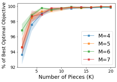
We proved in Appendix C that piecewise linear approximation guarantees improve with increasing . To choose a suitable K for our experiments, we varied the number of pieces () from 2 to 20 in steps of 2, and report the relevant statisitcs in Figure 3. We note that across various settings, the results have saturated by , and thus use for all our experiments.
Appendix L Converting Weighted Objective to MISOCP
Let
Further, let . Consider the stratified sampling objective
| (35) |
It is enough to show the conversion for the above as the clustering is a special case with for all . As before we substitute (notation is abused, but the constant subscript is and the variable subscript is ) for all and . Note that , and since , we have . Also, since then
Also, . The objective becomes . Thus, like the original (non-clustered) problem the objective is concave, and the only non-convexity is in the constraint , which can be approximated as earlier.
For MISOCP, we move the part of the objective becomes the linear function with an additional constraint that
| (36) |
(Recall r is the vector of all variables). The above is same as for the constant matrix (with entries or at appropriate entries) and constant vector c (with 1 in the component, rest 0’s) that picks the ’s and respectively.