The Born approximation in the three-dimensional Calderón problem II: Numerical reconstruction in the radial case
Abstract.
In this work we illustrate a number of properties of the Born approximation in the three-dimensional Calderón inverse conductivity problem by numerical experiments. The results are based on an explicit representation formula for the Born approximation recently introduced by the authors. We focus on the particular case of radial conductivities in the ball of radius , in which the linearization of the Calderon problem is equivalent to a Hausdorff moment problem. We give numerical evidences that the Born approximation is well defined for conductivities, and present a novel numerical algorithm to reconstruct a radial conductivity from the Born approximation under a suitable smallness assumption. We also show that the Born approximation has depth-dependent uniqueness and approximation capabilities depending on the distance (depth) to the boundary . We then investigate how increasing the radius affects the quality of the Born approximation, and the existence of a scattering limit as . Similar properties are also illustrated in the inverse boundary problem for the Schrödinger operator , and strong recovery of singularity results are observed in this case.
1. Introduction
Let be the ball of radius in with , and a bounded real non-negative conductivity such that holds in for some constant . For a given we consider the so-called Dirichlet to Neumann (DtN) map defined as
| (1.1) |
Here denotes the normal derivative at the boundary, and is the electrostatic potential given by the unique solution of the elliptic problem
| (1.2) |
The Calderón inverse problem consists in recovering the conductivity from the associated DtN (or voltage-to-current) map11 1 Since , a weak definition for must be given in place of (1.1). An appropriate definition follows from the weak formulation of the boundary problem (1.2).. This, now classical, inverse problem can be seen as a simplified mathematical model for Electrical Impedance Tomography (EIT), which is related to important applications in medical imaging, nondestructive testing and geophysics. See for example the references [ALMM+01, CIN99, IMNS06] for medical imaging applications.
From the mathematical point of view the first natural question is uniqueness, which consists in determining if the map is injective. Uniqueness was originally proved for conductivities by Sylvester and Uhlmann in [SU87] —see [CR16, Hab15] for lower regularity uniqueness results— and a stability estimate was given by Alessandrini in [Ale88].
Another important problem is reconstruction, where the aim is to design a method to recover from its associated DtN map. It is well known that the reconstruction problem is ill-posed due to the weak stability of the map . This means in particular that classical approaches based on least squares formulations are difficult to implement in practice. In dimension 3, a more successful attempt was addressed in the works [BKM11, DHK11, DHK12, DK14], where the authors implemented a direct reconstruction method, following the scheme proposed by Nachman in [Nac88]. However, the method is based on Complex Geometrical Optic solutions (CGOs) introduced in [SU87] and, as a consequence, it requires to solve a complicated integral equation on the boundary involving highly oscillating functions; therefore it presents a number of difficult challenges at the numerical level. We also refer to [MS20, MS12] for more references on the numerical aspects of EIT and for more information on the the two dimensional case that it is not addressed here.
For simplicity we assume for the moment that and that both and vanish at . Based on the works [SU87] and [Nac88], which give an explicit inverse formula for the map , it is natural to consider an approximation to that depends linearly on the DtN map. We will denote this approximation by , which formally is given by the formula
| (1.3) |
where (see Section 2 for a detailed discussion). Here, denotes the Fourier transform of a function defined as
The expression (1.3) has been considered in [BKM11] and a similar definition has been used in [KM11] as a way to obtain a numerical approximation to that avoids solving a boundary integral equation in order to reconstruct the boundary values of CGOs. The effectiveness of this linearization method has been recently compared to other reconstruction methods in [HIK+21] using synthetic data to simulate real discrete data from electrodes22 2 It is worth mentioning that in [BKM11, HIK+21] the notation is used for a different approximation that is not linear on , but is very similar in spirit to (1.3). The approximation (1.3) is denoted as in [BKM11]..
The fact that is linear on the data, makes a close analogue of the Born approximation in scattering problems for Schrödinger operators . For this reason from now on we will refer to as the Born approximation of . In scattering applications, the Born approximation is widely used as an acceptable approximation for the potential . It is well known, for example, that it contains the leading singularities of , and that one can reconstruct explicitly from its Born approximation in the case of small potentials. See, respectively, [Mer18, Mer19] and [BCLV18, BCLV19] for recent results on both questions and for further references. This suggest that could have similar numerical applications.
Unfortunately, the definition of in (1.3) is formal in two ways. On one hand, it is not clear if the limit in the right hand side exists. On the other hand, even if the term in the right hand side were a well-defined function, there is no guarantee that it decays in fast enough in order to ensure that it is the Fourier transform of a function. These issues, together with the lack of a simple procedure to obtain from —notice that (1.3) involves oscillatory integrals and a high frequency limit— has relegated the Born approximation to a marginal place in the numerical reconstruction aspect of the three-dimensional Calderón problem.
Recently, explicit formulas for the Born approximation of a closely related inverse problem —in which the elliptic operator in (1.2) is replaced by a Schrödinger operator — have been obtained in [BCMM21]. These formulas can be adapted to the conductivity inverse problem very easily, and show that the limit (1.3) exists when the conductivity is a sufficiently smooth radial function:
| (1.4) |
Moreover, they also show existence of the limit in the non-radial case after an appropriate average.
Considering radial conductivities provides an important simplification to the problem, since in this case the DtN map is a function of the spherical Laplacian on . As a consequence, is diagonal in the basis of spherical harmonics on . In fact, the eigenspaces of are precisely the spaces of spherical harmonics of a fixed degree . We denote by the sequence of eigenvalues of the DtN map in . One can show that (see for instance [BCMM21]), when one has and that the first eigenvalue always vanishes, that is . From now on we will drop the super-index in the case and use the notation .
A consequence of the results in [BCMM21] (see Section 2.3 for more details) is that for a radial conductivity as (1.4), and such that both and vanish at , one has:
| (1.5) |
with .
The series on the right hand side in (1.5) is absolutely convergent for all since , as follows from the min-max principle applied to the eigenvalues of the DtN map. However, (1.5) is still formal since we do not have a priori estimates that control the growth in the variable, necessary to define the inverse Fourier transform of (1.5) in a natural functional space.
On the other hand, we notice that the right hand side of (1.5) is well-defined for radial conductivities . As a consequence we will drop the regularity requirement (1.4) and assume just that where
The regularity condition close to the boundary is imposed beacuse the analysis requires that both and are well defined and vanish at .
In fact, in the numerical experiments in Section 3.3 the right hand side of (1.5) decays quickly for large , even for conductivities with jump discontinuities at the interior. This is an interesting fact since in principle the heuristic derivation of (1.3) requires conductivities with two bounded derivatives (1.4), and leads us to conjecture that is indeed always well defined for conductivities in . Notice also that this class is strictly larger than the one for which the uniqueness of the inverse problem is proved.
We have tested formula (1.5) in different situations with high precision values of to allow us to explore which features of can be recovered by . All the numerical experiments involve radial conductivities in . In particular we find:
- I)
Local uniqueness from the boundary. Assume that and are two different radial continuous conductivities. Then for implies that also for .
- II)
Approximation close to the boundary is in general a better approximation for in a region close to the boundary of the ball than close to the center of the ball. This is more or less independent of the size of , and only breaks down for very large conductivities. The fact that is a better approximation of when is close to the boundary has already been observed in [BKM11].
- III)
Approximation of small conductivities. As expected, is an excellent approximation for if is small, and the quality of the approximations provided by worsens as this difference becomes larger.
While property III) is to be expected, properties I) and II) are truly remarkable, and suggest that contains important information on the conductivity, even when the conductivities are not necessarily very close to . The numerical experiments made to study property I) have been motivated by [DKN21, Theorem 1.4] in which a uniqueness result that has an analogous locality behaviour from the boundary is proved. As far as we know these properties of the Born approximation do not have similar counterparts in inverse scattering problems. The particular case in property I) is rigorously shown to hold under the assumption that (2.6) is a tempered distribution (see Appendix A). Notice that this case implies the following property:
- IV)
Support from the boundary. If vanishes for then vanishes for .
Another very natural question in this context is to understand in which sense the Born approximation could recover the leading singularities of . Recovery of singularities results from the Born approximation are well known in Inverse Scattering, as mentioned previously. In the two-dimensional Calderón problem a detailed scheme to reconstruct the singularities from bounded conductivities has been given in [GLS+18], where is also noted that this question is relevant for medical applications of EIT (classifying strokes as ischemic or hemorrhagic, for instance, see references in [GLS+18]). In this work we are not able to capture numerical evidence of recovery of singularities for , though we get strong numerical evidence of this phenomenon when considering the inverse boundary problem for the Schrödinger operator . The numerical experiments presented in Section 3.4 show clearly that the Born approximation for this problem contains the same jump discontinuities of the original potential, even for very large potentials.
The Born approximation and formula (1.5) are useful to gain new insights on the reconstruction aspect of the Calderón problem. For notational simplicity let us illustrate this in the particular case . First, note that the Born approximation contains the same information as the DtN map since one can show that
| (1.6) |
under the assumption that is well defined33 3 This is true under the assumption that . To prove rigorously a weak version of (1.6) one has to show that is a tempered distribution for all for some . (see Section 2.4). This implies that formally determines , since determines the conductivity (at least in the appropriate function spaces where uniqueness holds). Thus, from the point of view of reconstruction, properties I)–III) imply that is an equivalent, but more useful, way to present the measurement data than the DtN map.
On the other hand, the Born approximation does not provide a way around the bad stability characteristic of the Calderón problem. In fact, the identity (1.6) implies that finding the Born approximation is essentially equivalent to solving a Hausdorff moment problem, which is also an ill-posed problem with logarithmic stability —see [DKN21] for more details on the relation between the moment problem and the radial Calderón problem. This instability is reflected in the numerical experiments: the implementation of formula (1.5) is not difficult but it requires very precise values of . In this work, the precision that we have used in the computation of the values of goes well beyond what one can expect in any real application, since one of the objectives is to gain insights on the general behaviour of .
The previous observations open an intriguing possibility. If one can obtain from the DtN map, and from , the reconstruction problem is factorized in a linear part and a non-linear part. The linear part is the Hausdorff moment problem that is formally solved by (1.5). This raises the question of understanding whether or not the actual stability estimate of the non-linear part is better than logarithmic. An affirmative answer to this question would imply that the bad stability properties of the radial Calderón problem are caused exclusively by the fact that one is implicitly solving a moment problem, and that the Born approximation has already made the hard work of decompressing the information contained in the DtN map. In this sense, numerical observations I)–III) about seem to give some evidence, albeit indirect and very limited, that this could be true. This will be discussed with more detail in Section 2.4.
Another interesting issue that is analyzed here is the dependence on of the quality of the Born approximation of a fixed conductivity that is defined on . Assume that is supported in . In principle (1.5) yields a different Born approximation for each value of . It is possible to find an identity relating the eigenvalues of of the DtN map in to the eigenvalues of the DtN map in (see Section 2.2). This yields the following formula
| (1.7) |
which taking the limit becomes
| (1.8) |
This identity shows that one can define a scattering limit for the Born approximation. The numerical experiments in Section 3 suggest that in general is a worse approximation for than if , but the deterioration stabilizes very quickly as grows, as suggested by formula (1.8). See Section 2.2 for more consequences of these formulas in the context of the inverse boundary problem for the Schrödinger operator .
Nonetheless, the Born approximation can be used as the basis of a simple but useful algorithm to reconstruct conductivities close to from the DtN map. Since is obtained after linearizing the Calderón problem around , one expects the difference between and to be of quadratic order in the norm of . This suggests that the following fixed point algorithm can be used to improve the Born approximation when the conductivities are close enough to :
| (1.9) |
We provide numerical evidence on the fast convergence for continuous conductivities that are not far from (see Section 4). Similar iterative algorithms have been used in scattering theory, see [BCR16, BCLV18]. In the context of the Calderón problem, see [GH22] for a recent reconstruction algorithm for small conductivities in dimension 2 in which convergence and stability are proved. Note that, in order to compute the new iteration in (1.9), we have to approximate the Born approximation of and this requires its DtN map. Therefore, the efficiency of the algorithm strongly depends on the existence of an accurate and fast algorithm to solve the direct problem, i.e. to compute the eigenvalues of from . Fortunately, in the case of radial conductivities such algorithm is available (see [BKM11]).
The rest of the article is divided as follows. In Section 2 we will introduce the Born approximation for the inverse boundary problem for the Schrödinger and we will analyze the scattering limit for this problem. We then show how to derive (1.5) and study the relation of the Born approximation with the inverse Hausdorff moment problem. In Section 3 we describe some implementation details to obtain the Born approximation and include the numerical experiments for the potential and for the conductivity problems. Finally in Section 4 we provide numerical evidence on the convergence of the numerical algorithm (1.9) and an analogous version of the algorithm for the Schrödinger operator . The Appendix A provides a short proof of property IV) under the assumption that the Born approximation is well defined as a tempered distribution.
Acknowledgments
This research has been supported by Grant MTM2017-85934-C3-3-P of Agencia Estatal de Investigación (Spain). The authors would like to thank Thierry Daudé and François Nicoleau for very insightful discussions on the radial Calderon problem.
2. Two closely related inverse problems
In this section we introduce the Born approximation for the inverse boundary problem associated to the Schrödinger operator in Section 2.1, and we analyze the scattering limit for this problem in Section 2.2. We then show how to derive (1.5) in Section 2.3. Finally in Section 2.4 we study the relation of the Born approximation with the inverse Hausdorff moment problem, and its implications for the numerical reconstruction in the Calderón problem.
2.1. The Born approximation in the inverse Schrödinger boundary value problem
In [SU87], Sylvester and Uhlmann showed in particular that determines for conductivities in by reducing the problem to an inverse boundary value problem for the Schrödinger operator . We next recall the main ingredients of their strategy. For with at the boundary, let
| (2.1) |
Then
| (2.2) |
if and only if satisfies (1.2).
Consider the family
| (2.3) |
Note that contains all the that are obtained from some via (2.1). Again, the DtN map associates to a function the normal derivative , where is the unique solution of (2.2). In particular, for as in (2.1) one has that
| (2.4) |
and hence whenever .
These observations show that the uniqueness and reconstruction questions for are reduced to the unique determination and reconstruction of a potential from the Dirichlet to Neumann map associated to the Schrödinger operator on .
Assume now that is a radial function such that , not necessarily arising from a conductivity via (2.1). For such , the DtN map is diagonal in the spherical harmonics. From now on we denote the eigenvalues of at by , and in the case .
In this inverse problem the Fourier transform of the Born approximation can be defined as the limit
| (2.5) |
where , as in the case of (1.3), see [BCMM21] for more details and references on the origin and motivation of this definition.
Recently, in [BCMM21, Theorem 1] the authors introduced an explicit formula for the Born approximation in the radial case when the domain is the unit ball :
| (2.6) |
An analogous but more complex formula is also proved for the non-radial case, see [BCMM21, Theorem 3].
As in the case of the conductivity, we remark that (2.6) is formal. If is supported in , it follows from [BCMM21, Theorem 2] that
| (2.7) |
for . This estimate implies that the series in (2.6) is absolutely convergent for all , but there is not an a priori control of the growth in the variable. This is a subtle problem that will be discussed again in Section 2.4.
Formula (2.6) provides an easy way to approximate the Born approximation numerically. As expected, the numerical results indicate that it shares many properties with the conductivity case:
- I.b)
For bounded potentials, the Born approximation is well defined as an inverse Fourier transform of (2.6) since decays to 0 as , provided that the potential has a not very large negative part . It is not clear if the Born approximation is well defined for very large and negative potentials, since in the numerical experiments (2.6) becomes very large and separates from as .
- II.b)
is in general a better approximation for in a region close to the boundary of the ball than close to the center of the ball.
- III.b)
As in the case of the conductivity, if and are two different potentials and for , it follows that for .
- IV.b)
The Born approximation recovers the jump discontinuities of . This is known as recovery of singularities and it is well established in other scattering problems, as mentioned in the introduction.
- V.b)
In most of the numerical examples, given a potential and a parameter , the Born approximation of develops a characteristic oscillatory behaviour close to as grows.
In analogy with the iterative algorithm (1.9), we propose the following algorithm to improve the Born approximation for the Schrödinger inverse boundary problem:
| (2.8) |
As we show in the numerical experiments below, this algorithm approximates very fast potentials that are not large in the norm.
2.2. The scattering limit
It is possible to extend the Born approximation (2.6) to a formula that is valid for any ball of radius . Let . We denote momentarily the DtN map of in by . For convenience, we will omit the superscript when as in the case of the eigenvalues. Also, we will denote in as and its Fourier transform by . The following identity for the Born approximation of a potential in follows from a straightforward change of variables in formula (2.6):
| (2.9) |
In fact, the change of variables , transform the initial problem (2.2) into the corresponding one for the unit ball with potential . Also, with this change of variables (2.5) implies that . This proves (2.9). Formula (1.5) for the conductivity follows easily by combining the formula (2.9) with the linearization of (2.1), as we will show in Section 2.3.
An interesting question is how the Born approximation of a fixed potential might depend on . That is, we want to compare the different Born approximations for the same potential . We start with the following simple lemma.
Lemma 2.1.
Let , , and , where is supported in . Assume that for all . Then the eigenvalues of in the unit ball determine the eigenvalues for all :
| (2.10) |
Proof.
Let be a spherical harmonic of order . Let be the solution of (2.2) with . Since the potential is radial, by separation of variables one has that , where is a solution of
| (2.11) |
Note that for every one has
Therefore, if , since is supported in we have that is a solution of the free equation in . It follows that
Since the restriction of to is also a solution of (2.11) with , by the previous discussion we have that
Hence we have the linear system
which can easily be solved to find and in terms of , , and . Then, plugging the solutions into the identity
yields formula (2.11) after some computations. ∎
As a consequence of this lemma, if , we can write (2.9) in terms of the eigenvalues of in the unit ball:
| (2.12) |
Therefore the limit of the previous expression is well defined:
| (2.13) |
This can be understood as a scattering limit for the Born approximation. Formulas (1.7) and (1.8) follow easily from the previous identities, as we will show in Section 2.3.
It is well known that the inverse boundary value problem for the Schrödinger operator is closely related to the fixed energy scattering problem as , see [Uhl92]. Therefore, the fact that is well defined opens the possibility of obtaining a Born approximation in terms of the fixed angle scattering data related to and formula (2.9) as .
Notice that the fact that is not linear on is a consequence of the non-linear identity (2.10) relating and . After linearizing (2.12) and (2.13) with respect the eigenvalues , one recovers exactly (2.6). As in the case of the conductivity, for a fixed potential we will later show numerically that becomes a worse approximation for as grows. This suggest that it is always a better strategy to obtain from with Lemma 2.1 and use (2.6) rather than using directly (2.9).
2.3. The formula for
Formula (1.5) follows from linearizing (2.2). First, we assume that . By (2.4) this implies that
| (2.14) |
where . The map is a non-linear map between and . It is not difficult to verify that the Fréchet derivative of this map at , is given by the operator . Thus
Since and have compact support, we can extend both functions to by zero and take the Fourier transform of the previous expression. This yields
where is some remainder term. Combining the linearization of the Schrödinger problem with the linearization
gives the following definition for :
| (2.15) |
This is essentially the same argument given in [BKM11] to motivate the definition of . Notice also that now (1.5) follows directly from and (2.9). In the same way, formulas (1.7) and (1.8) also follow immediately from (2.12) and (2.13).
Since is obtained from , in principle one requires the conductivity to have two bounded derivatives, but nothing prevents us to use (1.5) for less regular conductivities as mentioned in the introduction. In fact, one important advantage of (1.5) is that it does not require to go through the Schrödinger problem: it only involves the DtN map .
2.4. Connection with the Hausdorff moment problem
In this section we show that formula (2.6) implies that the linearization of the radial Calderón problem is essentially a Hausdorff moment problem, a connection observed in [DKN21] and [BCMM21]. To see this, let be any radial function with compact support. Define the moments
| (2.16) |
Then, it holds that
| (2.17) |
where the series on the right hand side converges absolutely for radial compactly supported —see [BCMM21, Section 3] for a short proof of this fact44 4 Notice that the compact support of is essential. It is not difficult to find counterexamples to this formula in the Schwartz class.. This means that formula (2.17) is a formal solution for the following Hausdorff moment problem: given a sequence of numbers , find a compactly supported and radial function such that (2.16) holds with .
The similarity between formulas (2.6) and (2.17) implies that the linearization of the radial Calderón problem is equivalent to the previous Hausdorff moment problem. In fact, formally one can think of as the radial and compactly supported function such that , provided that such a function exists.
On the other hand, if is supported in , it follows from [BCMM21, Theorem 2] that
| (2.18) |
for . An important consequence of this estimate is that the linear map is the Fréchet derivative of the non-linear functional on at . Thus, estimate (2.18) offers a different way to understand the connection between the radial Calderón problem and the Hausdorff moment problem. This has also been observed in a more general setting in [DKN21].
The same connection can be established in the case of the conductivity problem, as we saw in the introduction. To see this, we now justify identity (1.6). First, it is convenient to introduce the following notation. Let be the following operator:
where is a sequence of reals numbers belonging to . With this notation we can respectively write (2.6) and (2.17) as
The first identity together with (2.14) and (2.15) imply that
| (2.19) |
which is a completely equivalent way to write (1.5) in the case . From the previous expression identity (1.6) follows directly, provided that belongs to an appropriate functional space.
We have already mentioned that the definition of and is formal, since we do not control the growth of the right hand sides of (1.5) and (2.6). This question now becomes equivalent to the non-trivial matter of determining if is the moment sequence corresponding to a function (or distribution), and analogously for the conductivity. As we have already mentioned, the numerical experiments in this work suggest that this is the case for conductivities in , and for potentials satisfying certain conditions —see property I.b).
As mentioned previously, the problem of recovering a conductivity from the DtN map in the Calderón problem presents a number of numerical challenges. The Born approximations and offer a simpler setting in which study these problems, by giving an approximation to and , respectively, that can be computed easily from the spectrum of the DtN map, and which contains useful information on the conductivity or the potential. Nonetheless, the stability challenges that appear in the reconstruction problem also appear to compute the Born approximation as can be expected from the connection with the Hausdorff moment problem.
The Hausdorff moment problem is a notoriously ill-posed inverse problem, see for example [AGLT02]. In fact, it is related to the inversion of the Laplace transform, which is also an ill-posed problem (to see this, use the change of variables in the last integral of (2.16)). Analogously to the Calderón problem, the Laplace transform and the forward map in the Hausdorff moment problem are injective under suitable conditions, but the inverse mappings are not continuous. This affects stability, which can only be achieved in compact subspaces of potentials or conductivities. These are called conditional stability estimates, see [KRS21] for more details (see also [STY01], for conditional stability estimates for the inverse Laplace transform that are analogous to the usual stability estimates of the Calderón problem). In the Hausdorff moment problem one can expect also to have logarithmic stability estimates. One (rough) way to look at this is through (2.7): since the moments and have the same size, the arguments of [Man01] and [KRS21] should imply that the maps and have similar restrictions on possible conditional stability estimates.
As mentioned in the introduction, it is natural to ask if the hard and unstable part of decompressing the information from the DtN map is already been achieved by the formulas (1.5) and (2.6). This would be reflected in better stability estimates for the map , or for the map . The fact that the Born approximation in numerical experiments captures the high frequency part of the potential together with the values of close to the boundary, offers some indirect evidence that this could be true. Also, the Born approximation approximates very well small potentials (say, ) which also suggests better stability for with a smallness condition. From the point of view of the moments and the eigenvalues, (2.18) shows that the largest differences between them appear for low values of , which also could imply stability estimates better than logarithmic for the map . The same can be considered for the conductivity problem. All these questions remain open.
The instability of the moment problem is reflected in this work in the need of high precision computation of the values of in order to obtain accurate reconstruction of the high frequency part of and . In general to reconstruct and with (2.6) and (1.5) up to frequencies one has to sum the series up to . Thus, by (2.7), the relevant data is of order with if or are supported in (see more details in Section 3). As a consequence, recovery of the high frequency parts of and with formulas (1.5) and (2.6) using real data is a hard problem (note, however, that this difficulty is also present in the full reconstruction problem). On the other hand, the advantage of defining as the function that satisfies is that one does not need to apply necessarily (2.6), but use instead other numerical approaches to the moment problem.
As a consequence of the previous discussion, it is natural to expect that regularization techniques (see [AGLT02]) commonly used to deal with noisy and real experiment data will be necessary to obtain and . The need of regularization techniques can be seen in (1.5) and (2.6): a small perturbation of one of the eigenvalues adds a derivative of a distribution to and .
3. Numerical computation of the Born approximation
In this section we describe some implementation details to obtain the Born approximation and include numerical experiments both for the potential and conductivity problems when .
3.1. Computation of the DtN map
Let . The Born approximation formulas (1.5) and (2.6) and the reconstruction algorithms (1.9) and (2.8) require very accurate values of in the case of the conductivity, and in the case of the potential. In the second case, we compute these eigenvalues using the recursive algorithm described in [BCFN] for piece-wise constant radial potentials. In the case of the conductivity we use the algorithm given in [BKM11], again for piece-wise constant conductivities.
Due to the continuity of the DtN map with respect to the potential in the norm, we can approximate the DtN map of any continuous function from the one associated to a sufficiently close (in the norm) piece-wise constant function. We just take a uniform partition and approximate the conductivity (or the potential) by the function that takes, at each subinterval, the value at the middle point. In the examples below we have considered approximations with a uniform partition of up to 10,000 subintervals in .
Another important fact is the computer precision. As we describe below we consider eigenvalues in our experiments. However, since decays exponentially in , accurate approximations of these eigenvalues require more than the standard Float64 arithmetic precision. In our experiments we have considered up to Float1024 precision, according to the specific case.
3.2. Implementation details in the Born approximation
To compute the Born approximation we use formulas (2.6) for the potential and (1.5) for the conductivity problem. This requires a discrete inversion formula for the Fourier transform of radial functions, and an accurate approximation of the corresponding series. We discuss both issues below.
The inverse Fourier transform of a radial function can be approximated with the one-dimensional discrete inverse Fourier transform. In fact, if is a radial function and , the Fourier transform is given by
Let be the odd extension of to , that is . Then
where and stand, respectively, the one dimensional and the three dimensional Fourier transforms.
Analogously, one can write the three dimensional inverse Fourier transform in terms of the one dimensional inverse Fourier transform as follows. Since is radial, we have that for some function . Thus
where is again the extension .
In practice, we approximate a sampling of the function from a suitable sampling of its Fourier transform using the discrete inverse Fourier transform. To improve resolution we recover the extension of by zero to the interval , although we only draw the restriction to in the experiments below. Thus, a uniform sampling of in this interval with values is considered: with , . This requires a uniform sampling of in the interval with the same number of points, i.e. with , . As described in [BCR16, Lemma3] the convergence of this sampling to can be estimated in terms of the regularity of and its support, since an aliasing contribution appears for non-compactly supported functions in . In our case, we are not able to establish precise error estimates, since we lack precise estimates on smoothness and support of the Born approximation.
The second important issue is the approximation of the series, for example (2.6) in the case of the potential . Obviously, we only sum a finite number of terms. As described in [BCMM21] for any given the main contribution of this series is in the first terms . We observed that for the first terms in the series produce an stable approximation in the sense that adding more terms produces contributions of the order of to the Fourier transform in this interval.
On the other hand, note that the series in (2.6) contains very large terms for which the usual computer precision Float64 is not sufficiently good. In fact, this sum can only be computed accurately for with the standard precision. To obtain we considered Float1024 precision in our experiments.
The codes are programmed with Julia which is very efficient with arbitrary precision computations. They can be downloaded from [BCMM22].
3.3. Numerical experiments: The conductivity case
In this section we focus on the conductivity problem. We illustrate the main properties I)–IV) of the Born approximation with different experiments. In the first experiment we show that is defined even in the presence of jump discontinuities. The second experiment illustrates the local uniqueness from the boundary, that is, property I) in the introduction. Experiment 3 concerns the scattering limit of the Born approximation given by formula (1.8). Finally in experiment 4 we consider the Born approximation of different smooth conductivities: a conductivity close to , a very large conductivity and one degenerated example (a conductivity with reaches the value at the origin).
 |
 |
 |
 |
Experiment 1. We first consider two piece-wise constant conductivities (see Figure 1). This shows that the Born approximation is well defined even for conductivities with jump discontinuities. The lower simulation provides a better approximation of the potential since it is closer to the reference conductivity , which illustrates property III) in the introduction. Notice also that property IV) is verified in both examples.
Experiment 2. Here we illustrate the remarkable property I) of the Born approximation. In particular we observe that the Born approximations of different conductivities that coincide in an interval , also coincide in (see Figure 2). Notice that the Born approximations are much smoother than in the previous case, since there are no jump discontinuities in the conductivities. This experiment also shows that the Born approximation is better close to the boundary —property II)— and is a better approximation for conductivities closer to —property III).
 |
 |
Experiment 3. Here we compare the Born approximation given by (1.5) with , and the scattering limit given by formula (1.8) (see Figure 3). We take
We see that the scattering limit of the Born approximation deteriorates slightly with respect to but still recovers a fairly good approximation, in particular close to the boundary (in fact both and seem to satisfy property II)).
 |
 |
Experiment 4.
Here we consider the Born approximation for smooth conductivities. The simulations in the first row in Figure 4 correspond to the example considered in [BKM11] where the Fourier transform was computed only for due to numerical instabilities. Here we have circumvented these instabilities with higher machine precision. As illustrated by the second row in Figure 4, the Born approximation deteriorates as becomes very large, which is something to be expected since is constructed from a linearization at . The singular case illustrated in the third row of Figure 4 corresponds to a conductivity which is close to zero near . Observe that we still have a good approximation close to the boundary, but near the origin the Born approximation degenerates to negative values.
 |
 |
 |
 |
 |
 |
3.4. Numerical experiments: The potential case
In this section we focus on the potential case and again analyze the Born approximation through different experiments. The aim is to illustrate properties I.b)– V.b) of Section 2 and other similar phenomena. Experiments 5 and 6 illustrate the Born approximation for potentials of different sizes and regularities. Experiment 7 explores the depth dependence of the accuracy of the Born approximation by considering the approximation of a large set of randomly chosen potentials. In this way we can make a quantification of property II.b). In Experiment 8 below, we show that, when the potential is zero in a sufficiently large neighborhood of , the Born approximation is able to recover this value. Experiment 9 analyzes how the Born approximation of a fixed potential changes for different values of and in the scattering limit . Finally, in Experiment 10 we illustrate a particular oscillatory behavior associated to large negative potentials.
Experiment 5. Here we consider piece-wise constant radial potentials with two steps in the unit ball . We first compute the eigenvalues of the DtN map as described previously. From this sequence we have obtained the Born approximation according to formula (2.6). In Figure 5 and Figure 6 we compare the Born approximation and the potential, and their Fourier transforms.
In the first row of Figure 5 and the first two rows of Figure 6 we consider step potentials with . In these examples the Born approximation is a much better approximation close to the boundary of the ball than close to the origin, which illustrates property II.b). This property is also satisfied in the remaining cases, though the approximation deteriorates when the size of the potential increases. In particular, we observe that oscillations appear close to —property V.b)— for very large potentials, see the last rows of Figures 5 and 6.
We observe also a very clear recovery of singularities phenomenon —property IV.b). All the discontinuities of the step potentials are also present in the respective Born approximations, even for very large potentials. This is also appreciated in the Fourier transforms: large differences between the Fourier transform and the potentials are produced only for low frequencies.
 |
 |
 |
 |
 |
 |
| Potential | Fourier transforms |
In the particular case of Figure 6, we consider a bump type potential that vanishes in a neighborhood of . This fact seems to improve the behaviour of the Born approximation close to for medium and small size potentials. This phenomena will also be illustrated for a smooth potential (see experiment 8 below).
 |
 |
 |
 |
 |
 |
| Potential | Fourier transforms |
Experiment 6. This example (see Figure 7) is similar but now we consider a smooth function. In this case we do not have a explicit formula for the eigenvalues of the DtN map and we use an approximation with a piecewise constant function as described above. Again, the Born approximation is fairly good for a small potential (first row) and for a medium size potential it is a better approximation closer to the boundary (middle row) than close to the origin, which illustrates property II.b) in the smooth case. Again, for a large potential the low frequencies separate substantially at low frequencies (last row, right) and oscillations appear near .
 |
 |
 |
 |
 |
 |
| Potential | Fourier transforms |
Experiment 7. From the previous two examples we see that the Born approximation is more accurate close to the boundary. This is a general issue as illustrated in the next example (see Figure 8) where we have computed the error for a random sampling of potentials. We have chosen the potentials as linear combination of the first 20 trigonometric basis functions which are orthonormal in and satisfy the boundary conditions , i.e.
The Fourier coefficients are chosen randomly in the interval in such a way that . We observe that the error decrease as . We also illustrate the behavior of this error for larger potentials of the form , . In this case, the relative error , where , is close to zero near but becomes larger as approaches to . This is essentially a quantification of property II.b).

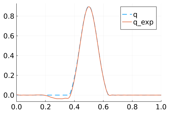
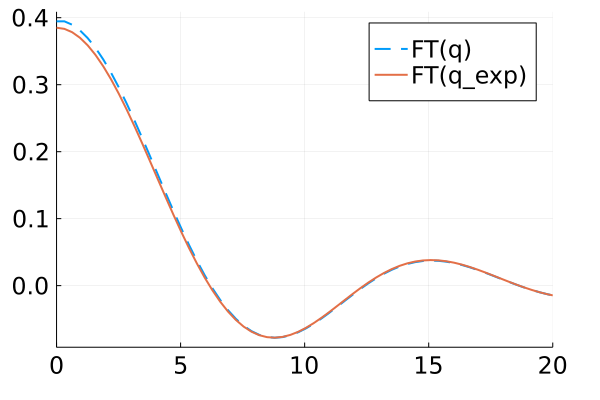
Experiment 8. An interesting feature appears when the potential is zero near . In this case, the Born approximation is somehow able of recovering this value as illustrated in the example in Figure 9 (see also Figure 6), at least if the potential is not too large. This seems to be very specific of the zero value since the error is in general much larger when the potential is not zero near , as illustrated in the previous experiment.
 |
 |
Experiment 9. In this example we consider the same potential in larger domains, i.e. we take as domain for (the case is the same as in Figure 7). We observe in Figure 10 that the Born approximation, given by (2.12), deteriorates but maintains a good approximation near . The case corresponds to the scattering limit given by formula (2.13).
 |
 |
 |
 |
Experiment 10. When the potential is negative the Born approximation seems to be less stable as shown in the experiment illustrated in Figure 11. As we increase the size of the potential Fourier transform of the Born approximation and the potential separate. This produces both oscillations and a singularity at in the Born approximation.
 |
 |
 |
 |
 |
 |
4. Iterative algorithm
In this section we illustrate the efficiency of the iterative algorithm described in (1.9) for the conductivity and in (2.8) for the potential.
Experiment 11. In Figure 12 we show the first iterations of the algorithm described in (1.9) when considering a Lipschitz conductivity and a smooth one. At each iteration the conductivity is better approximated. The behavior of the -error and -error are also illustrated in Figure 13. We observe that the rate of convergence depends on the regularity of . Note also that the piecewise constant conductivity considered in Experiment 1 above (in green-star) produces a decreasing error only for the norm. This is due to the Gibbs phenomenon which is present since we only compute a low pass filter of the conductivity.
 |
 |
 |
 |
Experiment 12. In Figure 14 we show the first iterations of the algorithm described in (2.8) when considering a discontinuous potential and a smooth one. At each iteration the approximation improves in a increasingly larger set. The behavior of the -error and -error are also illustrated in Figure 15. We observe that the smoothness of the potential affects to the error behavior. In fact, for the discontinuous potentials it stabilizes after a few iterations.
 |
 |
 |
 |
Appendix A Support of the Born approximation
Numerical results in Section 3 suggest that and are supported always in the same ball as, respectively, and . As far as we know this is a property that does not hold in inverse scattering problems where the Born approximation is commonly used. In the rest of this section we show a proof of this property provided that one assumes that formulas (2.6) or (1.5) give a tempered distribution.
We start by stating the following version of Paley-Wiener theorem.
Proposition A.1.
Let be a tempered distribution such that its Fourier transform has an holomorphic extension to all . Assume also that
for constants . Then is supported in , the ball of radius .
This version of Paley Wiener follows from [SW71, Theorem 4.9] by using an appropriate mollification of the tempered distribution .
We now reduce to the case for simplicity, since the higher dimensional cases follow with minimal modifications. Define the following holomorphic function in :
| (A.1) |
where the series is absolutely convergent by (2.7). The function is the holomorphic extension of from to .
Lemma A.2.
Let be a radial potential supported in . Then
| (A.2) |
where the implicit constants depends on .
Proof.
Combining Proposition A.1 with the previous lemma, we immediately obtain the following result.
Proposition A.3.
Let be a radial potential supported in . Assume that the the function given by (2.6) is a tempered distribution. Then is supported in .
Analogously one can prove the following proposition for the conductivity problem.
Proposition A.4.
Let be a radial conductivity such that is supported in . Assume that the function given by (1.5) is a tempered distribution. Then is supported in .
Proof.
It follows from Proposition A.1 and an estimate analogous to (A.2) for the analytic extension of . ∎
References
- [AGLT02] D. D. Ang, R. Gorenflo, V. K. Le, and D. D. Trong. Moment theory and some inverse problems in potential theory and heat conduction, volume 1792 of Lecture Notes in Mathematics. Springer-Verlag, Berlin, 2002. doi:10.1007/b84019.
- [Ale88] G. Alessandrini. Stable determination of conductivity by boundary measurements. Appl. Anal., 27(1-3):153–172, 1988. doi:10.1080/00036818808839730.
- [ALMM+01] M. Assenheimer, O. Laver-Moskovitz, D. Malonek, D. Manor, U. Nahaliel, R. Nitzan, and A. Saad. The t-SCANTMtechnology: electrical impedance as a diagnostic tool for breast cancer detection. Physiological Measurement, 22(1):1–8, feb 2001. doi:10.1088/0967-3334/22/1/301.
- [BCFN] J. A. Barceló, C. Castro, D. Faraco, and F. Ndiaye. Explicit formulas for the dirichlet to neuman map of the schrödinger operator with radial potentials in 3d. In preparation.
- [BCLV18] J. A. Barceló, C. Castro, T. Luque, and M. C. Vilela. A new convergent algorithm to approximate potentials from fixed angle scattering data. SIAM J. Appl. Math., 78(5):2714–2736, 2018. doi:10.1137/18M1172247.
- [BCLV19] J. A. Barceló, C. Castro, T. Luque, and M. C. Vilela. Corrigendum: A new convergent algorithm to approximate potentials from fixed angle scattering data. SIAM J. Appl. Math., 79(6):2688–2691, 2019. doi:10.1137/19M1278508.
- [BCMM21] J. A. Barceló, C. Castro, F. Macià, and C. J. Meroño. The born approximation in the three-dimensional calderón problem, 2021, arXiv:2109.06607.
- [BCMM22] J. A. Barceló, C. Castro, F. Macià, and C. J. Meroño. Born approximation in the calderon problem. https://github.com/carloscastroba/Born_approximation, 2022.
- [BCR16] J. A. Barceló, C. Castro, and J. M. Reyes. Numerical approximation of the potential in the two-dimensional inverse scattering problem. Inverse Problems, 32(1):015006, 19, 2016. doi:10.1088/0266-5611/32/1/015006.
- [BKM11] J. Bikowski, K. Knudsen, and J. L. Mueller. Direct numerical reconstruction of conductivities in three dimensions using scattering transforms. Inverse Problems, 27(1):015002, 19, 2011. doi:10.1088/0266-5611/27/1/015002.
- [CIN99] M. Cheney, D. Isaacson, and J. C. Newell. Electrical impedance tomography. SIAM Review, 41(1):85–101, 1999. doi:10.1137/S0036144598333613.
- [CR16] P. Caro and K. M. Rogers. Global uniqueness for the Calderón problem with Lipschitz conductivities. Forum Math. Pi, 4:e2, 28, 2016. doi:10.1017/fmp.2015.9.
- [DHK11] F. Delbary, P. C. Hansen, and K. Knudsen. A direct numerical reconstruction algorithm for the 3d calderón problem. Journal of Physics: Conference Series, 290:012003, apr 2011. doi:10.1088/1742-6596/290/1/012003.
- [DHK12] F. Delbary, P. C. Hansen, and K. Knudsen. Electrical impedance tomography: 3D reconstructions using scattering transforms. Appl. Anal., 91(4):737–755, 2012. doi:10.1080/00036811.2011.598863.
- [DK14] F. Delbary and K. Knudsen. Numerical nonlinear complex geometrical optics algorithm for the 3D Calderón problem. Inverse Probl. Imaging, 8(4):991–1012, 2014. doi:10.3934/ipi.2014.8.991.
- [DKN21] T. Daudé, N. Kamran, and F. Nicoleau. Stability in the inverse Steklov problem on warped product Riemannian manifolds. J. Geom. Anal., 31(2):1821–1854, 2021. doi:10.1007/s12220-019-00326-9.
- [GH22] H. Garde and N. Hyvönen. Linearised calderón problem: Reconstruction and lipschitz stability for infinite-dimensional spaces of unbounded perturbations, 2022, arXiv:2204.10164.
- [GLS+18] A. Greenleaf, M. Lassas, M. Santacesaria, S. Siltanen, and G. Uhlmann. Propagation and recovery of singularities in the inverse conductivity problem. Anal. PDE, 11(8):1901–1943, 2018. doi:10.2140/apde.2018.11.1901.
- [Hab15] B. Haberman. Uniqueness in Calderón’s problem for conductivities with unbounded gradient. Comm. Math. Phys., 340(2):639–659, 2015. doi:10.1007/s00220-015-2460-3.
- [HIK+21] S. J. Hamilton, D. Isaacson, V. Kolehmainen, P. A. Muller, J. Toivainen, and P. F. Bray. 3D electrical impedance tomography reconstructions from simulated electrode data using direct inversion and Calderón methods. Inverse Probl. Imaging, 15(5):1135–1169, 2021. doi:10.3934/ipi.2021032.
- [IMNS06] D. Isaacson, J. L. Mueller, J. C. Newell, and S. Siltanen. Imaging cardiac activity by the d-bar method for electrical impedance tomography. Physiological Measurement, 27(5):S43–S50, apr 2006. doi:10.1088/0967-3334/27/5/s04.
- [KM11] K. Knudsen and J. L. Mueller. The Born approximation and Calderón’s method for reconstruction of conductivities in 3-D. Discrete Contin. Dyn. Syst., Dynamical systems, differential equations and applications. 8th AIMS Conference. Suppl. Vol. II:844–853, 2011.
- [KRS21] H. Koch, A. Rüland, and M. Salo. On instability mechanisms for inverse problems. Ars Inveniendi Analytica, (paper nº7):93pp., 2021. doi:10.15781/c93s-pk62.
- [Man01] N. Mandache. Exponential instability in an inverse problem for the Schrödinger equation. Inverse Problems, 17(5):1435–1444, 2001. doi:10.1088/0266-5611/17/5/313.
- [Mer18] C. J. Meroño. Fixed angle scattering: recovery of singularities and its limitations. SIAM J. Math. Anal., 50(5):5616–5636, 2018. doi:10.1137/18M1164871.
- [Mer19] C. J. Meroño. Recovery of the singularities of a potential from backscattering data in general dimension. J. Differential Equations, 266(10):6307–6345, 2019. doi:10.1016/j.jde.2018.11.003.
- [MS12] J. L. Mueller and S. Siltanen. Linear and nonlinear inverse problems with practical applications, volume 10 of Computational Science & Engineering. Society for Industrial and Applied Mathematics (SIAM), Philadelphia, PA, 2012. doi:10.1137/1.9781611972344.
- [MS20] J. L. Mueller and S. Siltanen. The D-bar method for electrical impedance tomography—demystified. Inverse Problems, 36(9):093001, 28, 2020. doi:10.1088/1361-6420/aba2f5.
- [Nac88] A. I. Nachman. Reconstructions from boundary measurements. Ann. Math. (2), 128(3):531–576, 1988. doi:10.2307/1971435.
- [STY01] S. Saitoh, V. K. Tuan, and M. Yamamoto. Conditional stability of a real inverse formula for the Laplace transform. Z. Anal. Anwendungen, 20(1):193–202, 2001. doi:10.4171/ZAA/1010.
- [SU87] J. Sylvester and G. Uhlmann. A global uniqueness theorem for an inverse boundary value problem. Ann. of Math. (2), 125(1):153–169, 1987. doi:10.2307/1971291.
- [SW71] E. M. Stein and G. Weiss. Introduction to Fourier analysis on Euclidean spaces. Princeton Mathematical Series, No. 32. Princeton University Press, Princeton, N.J., 1971.
- [Uhl92] G. Uhlmann. Inverse boundary value problems and applications. Number 207, pages 6, 153–211. 1992. Méthodes semi-classiques, Vol. 1 (Nantes, 1991).