Turbulence Modeling of 3D High-speed Flows with Upstream-Informed Corrections
Abstract
Turbulence modeling has the potential to revolutionize high-speed vehicle design by serving as a co-equal partner to costly and challenging ground and flight testing. However, the fundamental assumptions that make turbulence modeling such an appealing alternative to its scale-resolved counterparts also degrade its accuracy for practical high-speed configurations, especially when fully 3D flows are considered. The current investigation develops a methodology to improve the performance of turbulence modeling for a complex Mach 8.3, 3D shock boundary layer interaction (SBLI) in a double fin geometry. A representative two-equation model, with low-Reynolds number terms, is used as a test-bed. Deficiencies in the baseline model are first elucidated using benchmark test cases involving a Mach 11.1 zero pressure gradient boundary layer and a Mach 6.17 flow over an axisymmetric compression corner. From among different possibilities, two coefficients are introduced to inhibit the non-physical over-amplification of (i) turbulence production and (ii) turbulence length-scale downstream of a shock wave. The coefficients rely on terms already present in the original model, which simplifies implementation and maintains computational costs. The values of the coefficients are predicated on the distribution of turbulence quantities upstream of the shock; this ensures that the modifications do not degrade the model predictions in simpler situations such as attached boundary layers, where they are unnecessary. The effects of the modifications are shown to result in significant improvements in surface pressure and wall heat flux for the 3D SBLI test case, which contains numerous features not observed in 2D situations, such as 3D separation, skewed boundary layers and centerline vortices. Considerations on the inflow values of turbulence variables and mesh resolution are provided
Keywords: Turbulence Modeling, Hypersonic
keywords
1 Introduction
With the renewed interest in hypersonic flight, cost-effective estimates of mean surface loading parameters such as pressure, skin friction coefficient, and heat transfer rates can significantly accelerate design evolution. High-fidelity numerical approaches such as Direct Numerical Simulations (DNS) and Large-Eddy Simulations (LES) are prohibitively expensive at high Reynolds numbers and remain well out of reach for practical systems for the foreseeable future; this motivates the continued vigorous development of Reynolds-Averaged Navier-Stokes (RANS) methods. RANS approaches have the potential to greatly reduce the considerable cost-function associated with the parametric analyses and optimization of hypersonic vehicle components, for which ground and flight testing is difficult and costly.
In addition to determining quantities of design interest, suitably tailored RANS can also provide insights into the unsteadiness of complex flow-fields (i) through various perturbation techniques (Ranjan et al. 2020; Prasad & Gaitonde 2022) and (ii) as an essential near-wall component of Wall-Modeled LES (WMLES) (Kawai & Larsson 2012) and Detached Eddy Simulations (DES) (Spalart 2009). These factors make RANS an attractive tool for the aerospace industry, as evident from its widespread adoption in commercial solvers.
Commonly used compressible RANS codes solve the Favre-averaged equations of motion. Favre-averaging gives rise to additional terms in the governing equations representing Reynolds stresses, turbulent heat flux, molecular diffusion and turbulent transport; these terms require the use of closure approximations through a turbulence model. The most widely used models involve closure approximations based on observations from equilibrium turbulent flat-plate boundary layer flows. Popular prescriptions include the use of Boussinesq approximation to model the Reynolds stresses, the application of strong Reynolds analogy to model the turbulent heat flux and the adoption of gradient approximations to model molecular diffusion and turbulent transport. These simplifying assumptions form the foundation of RANS and significantly reduce its computational requirement when compared to its high-fidelity counterparts. However, in practical high-speed flow configurations, where high heat transfer rates and shock boundary layer interactions (SBLI) are ubiquitous, these defining assumptions of RANS severely compromise its ability to capture experimentally measured behavior.
The degradation of RANS accuracy for practical high-speed configurations is well documented (Roy & Blottner 2006; Georgiadis et al. 2014; Coratekin et al. 2004), and several investigations have focused on improving predictions by examining the validity of these assumptions at high Mach numbers. For instance, Morgan et al. 2013 studied the Reynolds stress transport budgets in SBLI flows at Mach using a sequence of LES databases and argued that the inaccuracy of RANS stems from the inability of the Boussinesq approximation to represent the observed anisotropy in Reynolds stresses. They further indicated that although Reynolds stress transport (RST) models offered improved predictions than traditional eddy-viscosity-based turbulence models, their accuracy is still limited due to gradient approximations for turbulent transport. Zhang et al. 2021; Zhang et al. 2022 suggested a possible alternative to the RST-based-models by extending the application of a non-linear eddy-viscosity model (Craft et al. 2000) to hypersonic flows. Although the inclusion of non-linearity in Boussinesq approximation improved predictions, they observed a over-estimation of wall heat flux at Mach . This over-prediction in the heat flux was reduced to by introducing an additional source term in the governing equations (Zhang et al. 2022).
Xiao et al. 2007 took a fundamentally different approach to improve RANS heat transfer predictions by accounting for variable turbulent Prandtl number effects in RANS equations; the implication being that the strong Reynolds analogy is not valid across a shock wave (Mahesh et al. 1997). This idea of variable turbulent Prandtl number was further expanded to flows without shocks by Huang et al. 2020, who used DNS data of a Mach flow over a cooled flat plate to observe that the algebraic energy flux model by Bowersox & North 2010 gave a significantly improved prediction of the turbulent heat flux compared to the commonly used constant turbulent Prandtl number assumption.
In hindsight, it is rather unsurprising that RANS predictions can be improved by substituting one or more of its fundamental assumptions with extra transport equations (Xiao et al. 2007; Morgan et al. 2013; Vemula & Sinha 2017; Vyas et al. 2019) or phenomenological models (Vuong & Coakley 1987; Sinha et al. 2005; Pathak et al. 2018). Although extra transport equations can be more physically meaningful, their implementation in existing codes is not straightforward and invariably increases computational costs; this restricts the computational advantage offered by RANS. In contrast, phenomenological models are easier to implement and incur negligible extra costs, but their calibration in axisymmetric/2D problems usually does not extend accurately to 3D problems. The problem is further exacerbated because some prescriptions may have the potential to conflict with others, and improvement in predictions for one problem may be accompanied by a degraded performance in others. This has led to a confusing array of possibilities and has inhibited the effectiveness of RANS in sophisticated production suites.
This investigation aims to improve RANS predictions for 3D SBLI configurations at high Mach numbers without severely modifying the key assumptions responsible for the appeal of RANS techniques. Specifically, we seek corrections that (i) improve RANS predictions relative to existing approaches for flows where 3D features are dominant, (ii) do not degrade the performance in simpler cases where baseline RANS model is accurate, (iii) are straightforward to implement in existing RANS codes, and (iv) do not incur additional costs. We select the two-equation Launder and Sharma model (Gerolymos 1990) as a platform for further development; this selection is not restrictive based on its widespread availability in commercial solvers and its well known limitations in adverse pressure gradients (Rodi & Scheuerer 1986; Huang et al. 1994). A summary of the formulation is provided in 2.
The model is applied to a series of benchmark problems that collectively include the major phenomena expected in current and future hypersonic vehicles. We focus our attention on test cases in excess of Mach . Both two- and three-dimensional (2D, 3D) configurations are selected; a description of each of these test configurations and the underlying rationale for their selection is presented in 3. Each configuration is well documented and has a range of published data, either from experiments or benchmark higher-fidelity simulations. The performance of the baseline model for each test configuration is examined in 4. Special care is taken to ensure that the solution is independent of factors that have no direct connection to the model itself, such as grid resolution and freestream turbulence. Based on the performance of the baseline model, corrections are introduced to improve predictions. These corrections are carefully calibrated based on the upstream boundary layer to ensure they do not degrade the accuracy in other test cases where they are not necessary. Best practices for boundary conditions, mesh resolution and the use of corrections are documented to provide a degree of diagnostic analyses based on the phenomena of interest. Concluding remarks are made in 5.
2 Turbulence Model Formulation
Following Coakley & Huang 1992, a general two-equation turbulence model can be written in the framework of two variables, and as follows
| (1) |
where is the density, is the molecular viscosity and is the eddy viscosity. The subscript represents the equation for the corresponding turbulence variable . and are source terms whose general forms are given by
| (2) |
in terms of various constants , functions , and modeling parameters, . These source terms are a function of dilatation, , specific rate of dissipation and the strain invariant given by
| (3) |
The eddy viscosity, , in its general form can be written as
| (4) |
where, is the velocity scale and is a length scale that is determined by the variables and . The values of and the damping function also depend on this choice.
As stated previously, this investigation focuses on the Launder and Sharma model; this sets in eqn. 1. The length scale in eqn. 4 is now given by . The values of other model parameters are listed below in Table. 1.
All simulations are performed using an in-house finite difference solver that solves the full 3D Favre-averaged NS equations in generalized curvilinear coordinates. Steady state is achieved through time marching using an approximately factored (Pulliam & Chaussee 1981), implicit second-order Beam Warming scheme (Beam & Warming 1978). A third-order upwind biased Roe scheme (Roe 1981) is used for the inviscid fluxes with the van Leer harmonic limiter (Van Leer 1979), whereas the viscous fluxes are computed using a second-order central differencing scheme. All calculations use the ideal gas relation with air as a working fluid . The molecular viscosity is calculated using Sutherland’s law. The turbulent heat flux is modeled using the standard Reynolds analogy with a constant turbulent Prandtl number, . Details of the meshes and boundary conditions for each specific test case are presented in 4.
3 Test Configurations
The test cases are selected so that (i) they collectively exhibit a wide range of phenomena expected to occur in current and future high-speed vehicles, and (ii) have high-quality databases for validation in the form of benchmark DNS or experiments. The configurations are presented in Fig. 1, arranged in increasing order of complexity.


3.1 Flat Plate (FPM11)
The first test case shown in Fig. 1a corresponds to a Mach uniform flow over a cold flat plate at zero angle of attack. Accurate modeling of turbulent boundary layers subjected to wall cooling is critically important in the design of thermal protection systems. In addition, results from flat plate simulations are often required as inflow conditions for other hypersonic configurations of interest as shown later. These factors make the flow over a cooled flat plate an important step in assessing any turbulence model.
The freestream conditions are m/s, kg/m3 and K. The wall temperature is kept constant at K; these conditions are based on the measurements conducted as Calspan–University of Buffalo Research Center (CUBRC) (Gnoffo et al. 2013). This test case has been studied extensively in literature (Gnoffo et al. 2013; Rumsey 2010; Huang et al. 2020) to assess the performance of turbulence models and their corrections. The important parameters of interest are the shear stress and the heat transfer at the wall. This case is henceforth referred to as FPM11.
3.2 Long Cone Flare (LCFM6)
The second test configuration used in the present study consists of a long sharp cone with a downstream flare as shown in Fig. 1b. The long cone is representative of a hypersonic vehicle forebody (Wadhams et al. 2008) and allows for the development of a fully turbulent flow prior to an SBLI generated by the higher angle flare.
Similar compression corner flows have been used extensively in literature to test and improve turbulence model predictions (Xiao et al. 2007; Gnoffo et al. 2011; Wang et al. 2016; Pathak et al. 2018; Raje & Sinha 2021; Zhang et al. 2021; Zhang et al. 2022). This particular test case has been studied extensively for both laminar and turbulent conditions by Holden et al. 2018; the flow conditions used here correspond to “Run 33” in Holden et al. 2018. This test case comprises a Mach uniform flow at m/s, kg/m3 and K over the cone geometry. The wall temperature is kept constant at K. The key measurements are surface pressure and heat transfer. This case is referred to as LCFM6 in the manuscript.
3.3 Double Fin Configuration (DFM8)
The final test case consists of two identical fins mounted on a flat plate as shown in Fig 1c. The flow consists of an incoming Mach boundary layer at m/s, kg/m3 and K that interacts with the two shocks and other derivative features generated by the two fin surfaces. The wall temperature is kept constant at K based on the measurements of Kussoy et al. 1993 which are used for validation. We refer to this test case as DFM8 in the rest of the manuscript.
Such 3D SBLIs where the shocks due to one surface interact with a boundary layer on an adjacent surface are expected to be ubiquitous in hypersonic vehicle designs in both internal (scramjet flowpaths) and external (appendages) circumstances. The resulting flows of interest exhibit 3D flow separation, streamwise vortical structures, and complex shock/expansion systems, which involve efficiency degradation and even catastrophic unstart (Gaitonde 2015). Such interactions also play a crucial role in mode transition, such as ramjet to scramjet in dual-mode designs. Turbulence model modifications designed for 2D configurations (such as FPM11) do not extend to flows containing peculiarly 3D features. As elucidated later, the choice of DFM8 as a target flowfield of interest is motivated by the fact that it contains such features.
4 Results and Discussion
4.1 Baseline Results
We first assess the performance of the baseline model for each of the three test cases. As mentioned earlier in 1, errors in RANS predictions can occur due to grid resolution, inflow boundary conditions and turbulence model limitations. We first examine the effects of mesh resolution and the inflow turbulence on the FPM11 predictions. Three meshes are employed, details of which are documented in Table 2.
| Mesh | ||||
|---|---|---|---|---|
| Nominal | 0.24 | 0.001 | 1.26 | |
| Intermediate | 0.12 | 0.001 | 0.83 | |
| Fine | 0.06 | 0.001 | 0.41 |
The nominal mesh consists of and points in the streamwise and wall normal directions respectively. The two finer meshes are obtained by subsequently refining the nominal mesh in the and directions as shown in Table 2. The of the grid point adjacent to the wall at the plate center ranges from to for the three meshes. The solutions are marched to steady state using a non-dimensional time-step where m. Figure 2 compares the baseline predictions for the wall shear stress () and heat transfer () on the three meshes with DNS results of Huang et al. 2020 and experimental measurements (Gnoffo et al. 2013).
In general, the baseline model provides accurate estimates for both quantities once transition is obtained. The transitional behavior of the predictions can be linked to the tendency of type models to remain laminar at low Reynolds and high Mach numbers (Coakley & Huang 1992). The values of the in turbulent regime is independent of the mesh used, whereas becomes mesh independent once the value falls below unity. Once is achieved, further refinement only affects the location of transition and not the surface quantities after transition. It must be noted that such guidelines, although helpful in equilibrium situations, can be misleading in the presence of streamwise or spanwise gradients as the value of depends on the friction velocity on the surface. For flows with separation, this guideline becomes even more inapt as the friction velocity vanishes at the separation and reattachment points.
We now examine the effect of freestream turbulence on these predictions. In most RANS codes, the freestream turbulence is represented by specifying a turbulence intensity and an eddy viscosity ratio at the inlet boundary. Figure 3 shows the effect of varying these inflow turbulence values on FPM11 heat transfer predictions on the intermediate mesh.
The solid colored lines in Fig. 3a correspond to different inlet eddy viscosity ratios at an inflow turbulence intensity of , whereas the dotted lines indicate the evolution of along the plate length using the right axis. As expected, the transition location moves upstream when an increase in inflow turbulent viscosity. The maximum eddy viscosity experiences a sudden jump at the transition location as marked by the downward arrow in Fig. 3a for . As a general guideline, transition is achieved once the maximum eddy viscosity in the boundary layer crosses above 100; this guideline is used throughout this investigation to test for fully turbulent boundary layer in the subsequent test cases. Figure 3b shows the effect of increasing turbulent intensity on the predictions. For a constant value of 5, an increase in freestream turbulence intensity from to inhibits boundary layer transition and the flow remains laminar for the entire length of the plate. The maximum eddy viscosity in the laminar boundary layer barely rises above the value. Since the present focus is on predicting the turbulent quantities, this behavior is undesirable and can be circumvented by selecting a higher inlet eddy viscosity ratio of 10, which results in an earlier transition of the boundary layer despite increased turbulence intensity. Based on these observations, for flow over a cooled flat plate with no pressure gradients, the baseline model (without any corrections) is sufficient to provide accurate shear stress and heat transfer predictions provided an adequately high inflow turbulent viscosity is specified.
Figure 4 presents a schematic of the computational domain LCFM6 test case.

Due to the axisymmetric nature of the problem, a cylindrical coordinate system is chosen and only half the cone geometry is simulated using symmetry boundary conditions as shown. In order to ensure a turbulent boundary layer on the cone surface prior to the SBLI at the flare, a at turbulence intensity is specified at the inflow based on previous FPM11 results. The effect of mesh resolution is tested using three meshes, details of which are documented in Table 3.
| Mesh | ||||||
|---|---|---|---|---|---|---|
| Nominal | 0.12 | 0.912 | 0.8 | 0.001 | ||
| Intermediate | 0.08 | 0.631 | 0.4 | 0.001 | ||
| Fine | 0.07 | 0.508 | 0.3 | 0.0005 |
The nominal mesh consists of , and points in the streamwise, radial and circumferential directions respectively. The intermediate and fine grids are obtained by subsequently refining the nominal mesh along the three directions as shown. Based on prior results from the FPM11 test case, the mesh point closest to the cone surface in the turbulent boundary layer upstream of the flare is located at (calculated at m) for each of the three meshes. Here represents the normal distance from the wall. Figure 5 compares the resulting surface pressure and heat flux in the vicinity of the flare junction with experimental measurements for each of the three meshes.
The surface pressure predictions are independent of the mesh used, whereas the wall heat flux requires a significantly finer mesh to converge than that required for the FPM11 test case ( in the upstream attached boundary layer). Moreover, the model that provided very accurate results for the FPM11 test case, shows very little separation at the flare junction, resulting in an under-prediction of the peak surface pressure and a severe over-prediction in the peak surface heat flux. This is not unexpected, as it is well-known that the behavior of the model deteriorates even for incompressible adverse pressure gradient flows (Menter 1994). These deficiencies are addressed later in this section.
Figure 6 shows a schematic of the computational domain for the DFM8 test case. The incoming flow directed along the -axis with the -direction being the normal to the plate and the direction representing the spanwise direction. The fin leading edge is placed at . For computational efficiency only half the experimental domain is simulated.

Symmetry boundary conditions are applied at two planes as shown: the plane bisecting the two fins and the plane upstream of the leading edge. The freestream shock-structure comprising the primary shock (PS), the shoulder expansion (SE) and several reflected shocks (RS1 to RS3) are also shown for completeness. Three meshes are used to test for grid convergence; the details of each mesh are provided in Table 4.
| Mesh | |||||
|---|---|---|---|---|---|
| Nominal | 0.081 | 0.125 | 0.001 | 0.8 | |
| Intermediate | 0.051 | 0.085 | 0.001 | 0.4 | |
| Fine | 0.051 | 0.085 | 0.0005 | 0.3 |
These meshes collectively test the effect of streamwise, wall normal and spanwise spacing on predictions. Since it is already established that the model gives accurate predictions for flat plate boundary layer flows, the inflow boundary conditions are specified by matching the boundary layer momentum thickness of a precursor flat plate boundary layer simulation with the measurements of Kussoy et al. 1993 ; a comparison of the inflow quantities with that of Kussoy et al. 1993 is provided in Table 5 for completeness.
| / | / | / | ||
|---|---|---|---|---|
Figure 7 describes the 3D flow-field using streamlines, pressure gradient and Mach number contours at an artificial aspect ratio of to highlight different features under discussion that must be modeled.

A more detailed description of the flow-field can be found in Gaitonde et al. 1995. The freestream primary shock extends all the way down to the bottom plate, forming a succession of growing lambda shocks; three such shocks marked L1 to L3 are shown using pressure gradient contour lines. Each lambda shock is defined by its inviscid swept shock asymptote (shock tip) and the separation shock (shock edge) as marked in the top-right inset for shock L2. The incoming boundary layer separates along a line of coalescence formed by the lambda shock edges as shown. Separation is accompanied by a rapid increase in pressure which is maximum at the center symmetry plane. The bottom inset shows the flow structure in this plane using streamlines superimposed over Mach number contours. The primary incoming flow (highlighted using white arrows) separates at the point P1 (the point of intersection of the two lambda shock edges from each fin) and does not reattach to the plate throughout the computational domain. The region beneath the separated flow is occupied by the spanwise movement of the fluid from the fins towards the symmetry plane. This open mean flow structure is absent in 2D/axisymmetric cases like the LCFM6, which exhibits a closed separation bubble at the flare junction.
Figure 8 shows the surface pressure and the heat flux predictions along due to this interaction at the centerline on each of the three meshes.
The pressure and heat transfer values are normalized by N/m2 and W/m2 which are the reference quantities used in experiments. Similar to the LCFM6 test case, the surface heat flux requires a finer mesh for convergence in the incoming boundary layer than the surface pressure. Both quantities follow the same qualitative variation as the measured values. A key observation is the overprediction of the rise in surface heat flux due to the flow separation along the centerline. However, the over-prediction is less severe () than the LCFM6 test case due to the absence of a closed recirculation region as discussed previously. The initial pressure rise at (point P1) due to the intersecting lambda shocks is reasonably well predicted up to , beyond which the baseline model predicts much sharper rates of increase and decay cycles than the experiment.
4.2 Compressibility Correction
One of the key reasons for this degradation in accuracy for practical SBLI flows can be attributed to an over-amplification of turbulent kinetic energy immediately downstream of the shock (Sinha et al. 2003; Zhang et al. 2017). This results in a more energized boundary layer downstream of the shock than is physical; this delays, or in the case of LCFM6 completely inhibits separation. One method to improve the size of the separation bubble is to modify the coefficient in eqn. 2 to include the term as follows:
| (5) |
where is the turbulent Mach number. A value of reverts to the baseline model whereas an is equivalent to Sarkar’s compressibility correction (Sarkar et al. 1991), which, although developed primarily for free shear layers to address the dilatation dissipation term, has shown success in similar separated flows (Gaitonde et al. 2006). Figures 9a and 9b show the effect of employing this correction on the surface pressure and heat transfer for the LCFM6 test case.
With the use of this compressibility correction, the surface pressure predictions show a very good match in both the separation bubble size and the peak value with the measurements. This correction however, results in even higher values of the peak heat transfer ( over-prediction) than the baseline, though the location of the peak heat transfer matches that of the experiment.
Nonetheless, despite the improvement in surface pressure, the compressibility correction can alter the upstream equilibrium boundary layer, for which model coefficients were obtained without the compressibility correction. To show the effect of including this correction for attached flows, Fig. 9c displays results for the FPM11 test case with . The solid lines represent the wall shear stress along the plate whereas the dotted lines indicate the evolution of the maximum eddy viscosity using the right axis. The use of the compressibility correction results in a reduction of turbulent viscosity in the boundary layer; this explains the reason for the increase in separation size with for the LCFM6 test case, as shown previously. However, as shown in Fig. 9c, the reduction in eddy viscosity degrades the performance of the model in predicting the wall shear stress for FPM11. These observations highlight the underlying problem in turbulence modeling corrections where an improvement in one aspect is often accompanied by loss of accuracy in others. For the present investigation, it is therefore vital that modifications for one phenomenon not interfere with the accuracy of the baseline model for zero pressure gradient boundary layers.
4.3 Correction 1: Production Limiting
Keeping this constraint in mind, we investigate the terms on the right hand side of the equation. From eqn. 2, the right hand side for the equation can be expanded as
| (6) |
We define a non-dimensional parameter, given by
| (7) |
to examine the turbulence production to dissipation ratio for each test case. Figure 10a plots the variation of the maximum value of with streamwise distance for the LCFM6 configuration.

After an initial rise due to the oblique shock at the cone tip (), the coefficient drops to immediately at m, asymptotically approaching a value of in the fully turbulent boundary layer upstream of the flare. The interaction of this boundary layer with the shock at the flare results in a significant increase () in the value. Such high values represent a dominance of production over , resulting in a more energized boundary layer downstream of the shock which inhibits separation.
This observation indicates that surface predictions can be improved by preventing this nonphysical amplification in turbulence production downstream of the shock. A straightforward method to restrict this amplification is to place an upper bound on the value of based on a user-defined as follows:
| (8) |
where is the limited value which is substituted instead of in eqn. 6. The choice of dictates maximum value of turbulence production downstream of the shock. For example, a value implies no limitation on turbulence production and reverts back to the baseline model. Note, however, that eqn. 8 resembles the eddy viscosity limiting described in Menter 1994 and Kral et al. 1996 to eliminate unrealistic buildup of eddy viscosity in stagnation regions of airfoils (). Despite the fundamentally different direction of the present effort with these earlier studies, the use of this “production limiting” provides a degree of unifying context.
We take insights from the variation presented in Fig. 10a to select a suitable value. It is evident that for any in eqn. 8, the modified model behaves like its baseline variant upstream of the flare and therefore does not affect the attached boundary layer. Figure 10b shows the effect of incorporating this correction on the surface pressure predictions. Specifying a pre-defined improves the surface pressure predictions compared to the baseline. The separation bubble size and the peak pressure however, are still under-predicted; this suggests the use of a lower to further improve predictions. Based on Fig. 10a, any requires an additional geometric constraint of to avoid potential non-physical behavior near the oblique shock at the cone tip. For example, a , which is very close to the asymptotic in the attached boundary layer, can be employed for all m. The use of overpredicts the separation bubble size, resulting in higher peak pressures than the measurements. A value of 1.6 on the other hand, is found to be appropriate to accurately match the separation bubble size and peak pressure observed in the experiments. The peak heat transfer (shown in Fig. 10c), although smaller than the baseline model, remains overpredicted for . Despite this disagreement, the new predictions are highly encouraging because, unlike the compressibility correction, the modifications do not alter the upstream boundary layer, for which the baseline predictions are accurate. This is ensured by examining the eddy viscosity distribution upstream of the flare ( m) for the baseline and the modified variants () in Fig. 10d. The modified predictions shows identical eddy viscosity distribution in the attached boundary layer as the baseline, thus preserving the accuracy of predictions in the upstream boundary layer.
Figure 11 shows the effect of incorporating this correction on the centerline pressure and heat transfer for the DFM8 test case.
The threshold values of the parameter is calculated to be 1.381 in the inflow boundary layer. Since the inflow is specified from a precursor boundary layer simulation, a geometrical constraint is not necessary for this test case. The use of is observed to accurately capture the mean surface pressure along the centerline, including the pressure rise and peak pressure due to the PS interaction , the relief effect due to SE and the subsequent rise due the upstream influence of the RS2 interactions, with only modest disagreement between the secondary maxima and minima. Similar to the LCFM6 calculations, the peak heat transfer along the centerline remains over-predicted.
4.4 Correction 2: Length-scale Limiting
To improve heat transfer predictions, we take recourse to Reynolds 1980, who examined the role of turbulent dissipation in flows inside internal combustion engines. Based on the conservation of angular momentum, he argued that for flows undergoing rapid compression, is too slow to be of significance and could be neglected. Morel & Mansour 1982 expanded on Reynolds’ findings by modifying the equation to ensure a reduction in the turbulence length scale with an increase in density. This idea of length-scale limiting was extended to shock-induced compression by Vuong & Coakley 1987, who placed an upper bound on the turbulence length-scale to improve heat transfer for separated flows in the reattachment regime.
In the present investigation, we take a more generalized approach to Vuong and Coakley’s length-scale limiting by defining a non-dimensional parameter given by
| (9) |
Figure 12 shows the distribution of the maximum value of as a function of for the LCFM6 baseline calculations.
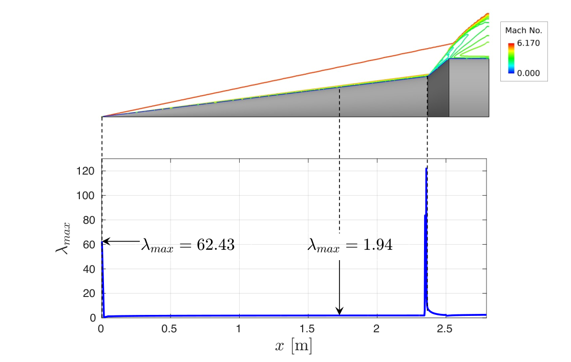
Similar to the variation in Fig. 10a, the oblique shocks at the cone tip and the flare are observed to amplify the value. After an initial value of due to the oblique shock at the cone tip, the value drops to zero at the very next axial location, approaching a value of in the attached boundary layer before being significantly amplified at the flare. This observation indicates that wall heat flux predictions can be improved by limiting this amplification of at the flare; this is achieved by placing an upper-bound on the turbulence length-scale as follows
| (10) |
where is a user-defined parameter. This length-scale is used to calculate as shown below
| (11) |
Based on the trends in Fig. 12a, the use of any (for all ) results in an value which is identical to the baseline model upstream of the flare; this preserves the accuracy of predictions in the attached boundary layer. Figures 12b and 12c show the heat transfer and surface pressure predictions for the LCFM6 test case at different values of . Contrary to production-limiting, the use of length-scale limiting has a significant effect on the heat transfer predictions. In general, the peak heat flux at the wall decreases with a decrease in value. The surface pressure is mostly unaffected except at very low values of . Figure 12d shows the eddy viscosity distribution in the attached boundary layer at m for all values tested. The perfect overlap of the length-scale limited simulations with the baseline indicates that the improvements in heat transfer are obtained without altering the upstream boundary layer.
Figure 13 shows the effect of incorporating this correction on the heat flux and surface pressure predictions for the DFM8 test case.
Based on a similar analysis as in Fig. 12a, the threshold value of is found to be in the inflow boundary layer when the distance is calculated from the bottom plate . A similar trend is observed, where a decrease in value decreases the peak heat transfer. The use of significantly improves heat transfer predictions, including peak heat transfer and the initial rate of increase along the centerline. Similar to the LCFM6 case, this correction has no effect on the surface pressure predictions. These observations are leveraged next to improve the overall predictions for the two test cases.
4.5 Combined Results: Production and Length-scale Limiting
The previous subsections have shown that the production and length-scale limiting corrections can independently improve surface pressure and wall heat flux without affecting the attached boundary layer. This subsection attempts to combine the two corrections to improve the overall predictions.
We first focus on the LCFM6 test case. Figure 14 shows the surface pressure and heat transfer predictions with and .
Note that, showed the best pressure predictions but significantly over-predicted the heat transfer for this test case (Fig. 10). When combined with length-scale limiting, the modified model accurately capture the separation bubble size and the reattachment peak pressure observed in measurements irrespective of the value; this observation indicates that the two corrections do not conflict with one another for this test case. For surface heat transfer, the modified predictions improve considerably compared to the baseline. The use of accurately matches the rate of increase in until m with a over-prediction in the peak value. In contrast, the use of accurately predicts the peak heat flux with an average under-prediction in the region . In both cases, the location of the peak heat transfer is correctly predicted. These results are highly encouraging as these improvements are obtained without altering the upstream attached boundary layer. Moreover, since the terms required to implement these corrections are already present in the baseline model, these modifications are straightforward to implement in existing codes and do not incur any additional computational cost. As an example, both the baseline and modified ( ) calculations for the LCFM6 test case required approximately CPU hours with 192 Intel® Xeon® 8268s Skylake ( GHz) processors ( hours of wall-clock time) on the intermediate mesh (Table 3).
We now focus our attention to the more complicated DFM8 test case. Figure 15 shows the predicted surface pressure and heat transfer rates along the centerline for the DFM8 test case with and .
Note that, and provided the best surface pressure and heat transfer predictions when applied independently (Figs. 10a and 12a). When combined, the use of is observed to accurately capture the mean surface pressure along the centerline, including the initial pressure rise and peak pressure, the relief effect downstream of the PS and the subsequent rise due the upstream influence of the RS2 interactions, with only modest disagreement at the secondary maxima. This correction combination however, only improves the surface heat flux in the range. The peak heat flux, similar to the baseline is over-predicted by . A further reduction in the value of at does not reduce the over-prediction in peak heat transfer rates. In fact, the best overall predictions are obtained by choosing a higher value of while keeping as shown. The peak heat transfer now shows only a over-prediction from the measured values without sacrificing the accuracy of surface pressure.
This deviation from the expected behavior indicates that the two modifications interfere with one another for the more complicated 3D case; this warrants a closer look at the flow-field for the two calculations. Figure 16 compares the streamlines (colored with P/P) in the proximity of the bottom plate for and with the baseline calculation.


Based on the description by Gaitonde et al. 1995, the experimentally observed indicators of 3D separation can be identified based on the streamline structure. The principle line of separation (PLS) is the line of coalescence joining the lambda shock edges (Fig. 7). The incoming flow separates along the line PLS as discussed earlier. The region beneath the separated flow is occupied by the spanwise movement of the fluid from the line of primary attachment (LPA) near the fin surface. The fluid emanating from the line LPA also forms another line of coalescence called the line of secondary separation (LSS) between the symmetry plane and the fin surface. As expected, the flow along the lines LPA and LSS is accompanied by an adverse pressure gradient. Interestingly, the spanwise movement of the fluid from the line LPA towards the symmetry plane and the line LSS is initiated with a favorable pressure gradient near LPA. For the baseline case, the line LSS asymptotically approaches the center symmetry plane with increase in downstream distance. For the case which gives accurate surface pressure predictions but overpredicts heat transfer, the distance between the line LSS and the symmetry plane is larger than the baseline. This suggests that less influence of the line LSS on the symmetry plane might be responsible for the accurate centerline pressure predictions. However, due to this increased distance, the line LSS now interacts with the line LPA near the shoulder. Because the value of used in the length-scale limiting is calibrated based on distance from the bottom plate (coordinate), the interaction of the lines LSS with LPA near the shoulder may result in a localized dominance of spanwise length-scales; this reduces the effectiveness of coordinate based limiting. Specifying a slightly higher value circumvents this complication as shown. The combination of predicts a footprint where LSS does not interact with the LPA while being at a sufficient distance from the symmetry plane. This results in the best simultaneous surface pressure and heat transfer predictions.
For completeness, Fig. 17 presents the spanwise surface pressure and heat flux predictions along the dashed vertical lines P and Q (see Fig. 16b) respectively.
The use of significantly improves the surface predictions along the span when compared to the baseline model. Similar to the LCFM6 test case, these improvements are obtained at the same computational cost as the baseline calculations ( CPU hours with processors). This is highly encouraging and demonstrates that including these simple limiting coefficients can significantly improve predictions from existing RANS codes while retaining the original computational efficiency. Moreover, since the terms used to incorporate these corrections are derived from a general two-equation model formulation ( ), the analysis can be easily extended to other two-equation turbulence models.
As a final point, we note that although the upstream boundary layer dictates the threshold values of and , coefficients derived for a given test case may apply for small variations in flow parameters, and are thus suitable for trend studies. However, a general recommendation for values of RANS coefficients remains an open question, especially for the rich variety of features encountered in 3D flows.
5 Conclusion
This investigation presents a methodology to improve the performance of the standard turbulence model for a series of increasingly complicated test cases that exhibit flow phenomenon expected to occur in the current and future hypersonic vehicles. For a Mach zero pressure gradient flow over a highly cooled flat plate, the baseline model yields very accurate estimates of surface shear stress and heat transfer rate. However, the results show different transition locations depending on the parameters chosen. A high inlet turbulent viscosity ratio overcomes the problem of the boundary layer avoiding transition. When applied to more complicated shock boundary layer interaction (SBLI) cases, the baseline model under-predicts the size of the separation zone leading to incorrect predictions of heat transfer and surface pressure. The use of a compressibility correction significantly improves surface pressure predictions by reducing eddy viscosity in the upstream boundary layer. However, the correction degrades performance for the flat plate boundary layer flow. To circuvent this limitation, two coefficients are introduced that independently control the amplification of turbulence production and the turbulent length-scale downstream of a shock wave. The values of these limiting coefficients are carefully chosen based on the information from the upstream boundary layer; this allows the modified model to retain its accuracy in zero pressure gradient boundary layers while significantly improving predictions in the presence of shock waves. For a Mach flow over a cone with a flare, the modified model accurately predicts the separation bubble size and the peak pressure, with only a modest disagreement in the wall heat flux. When applied to the more complicated, three-dimensional Mach flow in a double fin geometry, improved results for surface pressure and heat transfer are obtained along the centerline as well as along the span. The simplicity of these modifications allows a straightforward implementation in any existing code, while retaining the same computational cost. Currently, efforts are focused on exploring a general recommendation for the optimal values of these coefficients based on a range of Mach numbers.
Acknowledgements
This work was performed in part under the sponsorship of the DoD HPCMP Hypersonic Vehicle Simulation Institute with Dr. R. Cummings (USAFA) serving as Project Monitor. DVG also acknowledges partial support from the Collaborative Center for Aeronautical Sciences. The views and conclusions contained herein are those of the authors and do not represent the opinion of USAFA or the U.S. government. The authors are grateful for computational resource grants from the DoD HPCMP and the Ohio Supercomputer Center.
References
- Beam & Warming (1978) Beam, R. M. & Warming, R. 1978 An implicit factored scheme for the compressible navier-stokes equations. AIAA journal 16 (4), 393–402.
- Bowersox & North (2010) Bowersox, R. D. & North, S. W. 2010 Algebraic turbulent energy flux models for hypersonic shear flows. Progress in Aerospace Sciences 46 (2-3), 49–61.
- Coakley & Huang (1992) Coakley, T. & Huang, P. 1992 Turbulence modeling for high speed flows. In 30th Aerospace Sciences Meeting and Exhibit, p. 436.
- Coratekin et al. (2004) Coratekin, T., Van Keuk, J. & Ballmann, J. 2004 Performance of upwind schemes and turbulence models in hypersonic flows. AIAA journal 42 (5), 945–957.
- Craft et al. (2000) Craft, T., Iacovides, H. & Yoon, J. 2000 Progress in the use of non-linear two-equation models in the computation of convective heat-transfer in impinging and separated flows. Flow, Turbulence and Combustion 63 (1), 59–80.
- Gaitonde et al. (2006) Gaitonde, D., Kimmel, R., Jackson, D. & Zhong, X. 2006 Cfd analysis in development of flight test article for basic research. In 14th AIAA/AHI Space Planes and Hypersonic Systems and Technologies Conference, p. 8085.
- Gaitonde et al. (1995) Gaitonde, D., Shang, J. & Visbal, M. 1995 Structure of a double-fin turbulent interaction at high speed. AIAA journal 33 (2), 193–200.
- Gaitonde (2015) Gaitonde, D. V. 2015 Progress in shock wave/boundary layer interactions. Progress in Aerospace Sciences 72, 80–99.
- Georgiadis et al. (2014) Georgiadis, N. J., Yoder, D. A., Vyas, M. A. & Engblom, W. A. 2014 Status of turbulence modeling for hypersonic propulsion flowpaths. Theoretical and Computational Fluid Dynamics 28 (3), 295–318.
- Gerolymos (1990) Gerolymos, G. 1990 Implicit multiple-grid solution of the compressible navier-stokes equations using k-epsilon turbulence closure. AIAA journal 28 (10), 1707–1717.
- Gnoffo et al. (2011) Gnoffo, P., Berry, S. & Van Norman, J. 2011 Uncertainty assessments of 2d and axisymmetric hypersonic shock wave-turbulent boundary layer interaction simulations at compression corners. In 42nd AIAA Thermophysics Conference, p. 3142.
- Gnoffo et al. (2013) Gnoffo, P. A., Berry, S. A. & Van Norman, J. W. 2013 Uncertainty assessments of hypersonic shock wave-turbulent boundary-layer interactions at compression corners. Journal of Spacecraft and Rockets 50 (1), 69–95.
- Holden et al. (2018) Holden, M. S., Carr, Z. R., Wadhams, T. P. & MacLean, M. 2018 Measurements in regions of shock wave/turbulent boundary layer interaction with large shock generator/hollow cylinder and hollow cylinder/cavity configurations at mach numbers between 5 and 7 at flight matched enthalpies and in cold flows. In 22nd AIAA International Space Planes and Hypersonics Systems and Technologies Conference, p. 5198.
- Huang et al. (2020) Huang, J., Nicholson, G. L., Duan, L., Choudhari, M. M. & Bowersox, R. D. 2020 Simulation and modeling of cold-wall hypersonic turbulent boundary layers on flat plate. In AIAA Scitech 2020 Forum, p. 0571.
- Huang et al. (1994) Huang, P., Bradshaw, P. & Coakley, T. 1994 Turbulence models for compressible boundary layers. AIAA journal 32 (4), 735–740.
- Kawai & Larsson (2012) Kawai, S. & Larsson, J. 2012 Wall-modeling in large eddy simulation: Length scales, grid resolution, and accuracy. Physics of Fluids 24 (1), 015105.
- Kral et al. (1996) Kral, L. D., Mani, M. & Ladd, J. A. 1996 Application of turbulence models for aerodynamic and propulsion flowfields. AIAA journal 34 (11), 2291–2298.
- Kussoy et al. (1993) Kussoy, M., Horstoman, K. & Horstman, C. 1993 Hypersonic crossing shock-wave/turbulent-boundary-layer interactions. AIAA journal 31 (12), 2197–2203.
- Mahesh et al. (1997) Mahesh, K., Lele, S. K. & Moin, P. 1997 The influence of entropy fluctuations on the interaction of turbulence with a shock wave. Journal of Fluid Mechanics 334, 353–379.
- Menter (1994) Menter, F. R. 1994 Two-equation eddy-viscosity turbulence models for engineering applications. AIAA journal 32 (8), 1598–1605.
- Morel & Mansour (1982) Morel, T. & Mansour, N. 1982 Modeling of turbulence in internal combustion engines. Tech. Rep.. SAE Technical Paper.
- Morgan et al. (2013) Morgan, B., Duraisamy, K., Nguyen, N., Kawai, S. & Lele, S. 2013 Flow physics and rans modelling of oblique shock/turbulent boundary layer interaction. Journal of Fluid Mechanics 729, 231–284.
- Pathak et al. (2018) Pathak, U., Roy, S. & Sinha, K. 2018 A phenomenological model for turbulent heat flux in high-speed flows with shock-induced flow separation. Journal of Fluids Engineering 140 (5).
- Prasad & Gaitonde (2022) Prasad, C. & Gaitonde, D. V. 2022 A time-domain linear method for jet noise prediction and control trend analysis. Aerospace Science and Technology p. 107377.
- Pulliam & Chaussee (1981) Pulliam, T. H. & Chaussee, D. 1981 A diagonal form of an implicit approximate-factorization algorithm. Journal of Computational Physics 39 (2), 347–363.
- Raje & Sinha (2021) Raje, P. & Sinha, K. 2021 Anisotropic sst turbulence model for shock-boundary layer interaction. Computers & Fluids 228, 105072.
- Ranjan et al. (2020) Ranjan, R., Unnikrishnan, S. & Gaitonde, D. 2020 A robust approach for stability analysis of complex flows using high-order navier-stokes solvers. Journal of Computational Physics 403, 109076.
- Reynolds (1980) Reynolds, W. 1980 Modeling of fluid motions in engines-an introductory overview. Combustion modeling in reciprocating engines .
- Rodi & Scheuerer (1986) Rodi, W. & Scheuerer, G. 1986 Scrutinizing the k- turbulence model under adverse pressure gradient conditions. Transactions of the ASME 108, 174–179.
- Roe (1981) Roe, P. L. 1981 Approximate riemann solvers, parameter vectors, and difference schemes. Journal of computational physics 43 (2), 357–372.
- Roy & Blottner (2006) Roy, C. J. & Blottner, F. G. 2006 Review and assessment of turbulence models for hypersonic flows. Progress in Aerospace Sciences 42 (7-8), 469–530.
- Rumsey (2010) Rumsey, C. L. 2010 Compressibility considerations for kw turbulence models in hypersonic boundary-layer applications. Journal of Spacecraft and Rockets 47 (1), 11–20.
- Sarkar et al. (1991) Sarkar, S., Erlebacher, G., Hussaini, M. Y. & Kreiss, H. O. 1991 The analysis and modelling of dilatational terms in compressible turbulence. Journal of Fluid Mechanics 227, 473–493.
- Sinha et al. (2003) Sinha, K., Mahesh, K. & Candler, G. V. 2003 Modeling shock unsteadiness in shock/turbulence interaction. Physics of fluids 15 (8), 2290–2297.
- Sinha et al. (2005) Sinha, K., Mahesh, K. & Candler, G. V. 2005 Modeling the effect of shock unsteadiness in shock/turbulent boundary-layer interactions. AIAA journal 43 (3), 586–594.
- Spalart (2009) Spalart, P. R. 2009 Detached-eddy simulation. Annual review of fluid mechanics 41, 181–202.
- Van Leer (1979) Van Leer, B. 1979 Towards the ultimate conservative difference scheme. v. a second-order sequel to godunov’s method. Journal of computational Physics 32 (1), 101–136.
- Vemula & Sinha (2017) Vemula, J. B. & Sinha, K. 2017 Reynolds stress models applied to canonical shock-turbulence interaction. Journal of Turbulence 18 (7), 653–687.
- Vuong & Coakley (1987) Vuong, S. & Coakley, T. 1987 Modeling of turbulence for hypersonic flows with and without separation. In 25th AIAA Aerospace Sciences Meeting, p. 286.
- Vyas et al. (2019) Vyas, M. A., Yoder, D. A. & Gaitonde, D. V. 2019 Reynolds-stress budgets in an impinging shock-wave/boundary-layer interaction. AIAA Journal 57 (11), 4698–4714.
- Wadhams et al. (2008) Wadhams, T., Mundy, E., MacLean, M. & Holden, M. 2008 Pre-flight ground testing of the full-scale hifire-1 vehicle at fully duplicated flight conditions: Part ii. In 46th AIAA Aerospace Sciences Meeting and Exhibit, p. 639.
- Wang et al. (2016) Wang, L., Xiao, L. & Fu, S. 2016 A modular rans approach for modeling hypersonic flow transition on a scramjet-forebody configuration. Aerospace Science and Technology 56, 112–124.
- Xiao et al. (2007) Xiao, X., Hassan, H., Edwards, J. & Gaffney Jr, R. 2007 Role of turbulent prandtl numbers on heat flux at hypersonic mach numbers. AIAA journal 45 (4), 806–813.
- Zhang et al. (2021) Zhang, H., Craft, T. & Iacovides, H. 2021 The formulation of the rans equations for supersonic and hypersonic turbulent flows. The Aeronautical Journal 125 (1285), 525–555.
- Zhang et al. (2022) Zhang, H., Craft, T. & Iacovides, H. 2022 Application of linear and nonlinear two-equation turbulence models in hypersonic flows. AIAA Journal pp. 1–15.
- Zhang et al. (2017) Zhang, Z., Gao, Z., Jiang, C. & Lee, C.-H. 2017 A rans model correction on unphysical over-prediction of turbulent quantities across shock wave. International Journal of Heat and Mass Transfer 106, 1107–1119.