Biological Evolution and Genetic Algorithms
Exploring the Space of Abstract Tile Self-Assembly

The fundamental genetic dynamics of populations of living organisms are constrained by the mechanisms of Darwinian evolution (Dobzhansky 1973). Modern science motivates the detailed investigation of evolutionary processes, e.g. designing vaccinations often requires the understanding of how pathogens will evolve in the future (Domingo et al. 2001). According to Darwin, the fitness of an individual is a measure of its fecundity, i.e. the ability of its phenotype to reproduce (Darwin 2003). The phenotype of an organism is the composite of all of its observable traits (Hartl & Clark 2007). Neglecting environmental influences, all information about a phenotype is encoded in the corresponding genome, or genotype (Hartl & Clark 2007). Evolution may be understood as the process of adaptation of a population to peaks on a high-dimensional fitness landscape (Wright 1932; Gavrilets 1997).

Whether adaptation occurs is governed by the ratio of exploration to exploitation exerted by the biological operators driving the traversal of the fitness landscape: Exploration arises due to random mutation and recombination of genomic information, exploitation through natural selection. If exploitation dominates, disconnected peaks may never be discovered. If, however, exploration dominates, the trajectory through the fitness landscape resembles a random search, unable to adapt to localised features (M.A.Nowak 2006). Many fitness landscapes only allow adaptation below a critical mutation rate, called the error threshold (M.A.Nowak 2006). The evolution of an individual genotype, rather than a whole population, may be characterised by the accessibility of its immediate fitness landscape neighbourhood through mutation.

To this end, we define robustness to be the proportion of single mutations that don’t change phenotype, and evolvability to be the number of different phenotypes accessible under a single mutation (Wagner 2008). In conclusion, the key results of genetic dynamics are encoded in the topology of the underlying fitness landscape (M.A.Nowak 2006). Therefore, identifying a reasonable genotype$\rightarrow$phenotype map is essential. We now investigate such a map based on the dynamics of molecular self-assembly which is suitable for the description of the assembling protein quaternary structures, such as the shell of a virus (Johnston 2010).

A ubiquitous way by which complex physical structures emerge is through the self-assembly of simple subunits (Whitesides & Grzybowski 2002). For example, protein subunits assemble into the required quaternary structures for a particular function. Knowing how biology evolves the rule sets to self-assemble structures is therefore crucial to understand the evolution of simple organisms, such as viruses(Domingo et al. 2001). Self-assembly processes are difficult to observe experimentally due to its short length and time scales, therefore computational simulation may be an important source of insight (Johnston 2010).

The computational intractability and incomplete knowledge of many atomistic details motivates the development of coarsegrained models of self-assembly which attempt to capture the essential physics while retaining tractability (Johnston 2010). Johnston 2010 suggest an abstract model of self-assembly based on work by Winfree et al (Rothemund & Winfree 2000). This model, which we from now on refer to as JaTAM, exhibits rich phenotypic phenomenology and therefore promises to capture a lot of characteristics of general self-assembly processes(Johnston 2010). These characteristics include the correlation between decreasing occurence frequency with increasing structural complexity found in natural proteins, as well as the mutability of assembled structures (Ahnert et al. 2009).

The model’s building blocks consist of squares with labelled edges which are assembled on a planar grid according to fixed interaction rules. Squares are chosen from an inexhaustible library of tile types called a tile set, of which the first tile is placed first in the assembly process. Interaction rules state that labels bind in pairs, i.e. $1\leftrightarrow 2$, $3\leftrightarrow 4$ etc. except for label $0$, which is generally inert. Non-bonding label combinations neither repel nor attract. Binding is thermodynamically irreversible, which is reasonable if thermodynamic noise is much smaller than interaction strengths between subunits.

Tiles may be rotated orthogonally, but not flipped. The particular choice of interaction matrix differs from Winfree’s original model and results in a higher ratio of structures exhibiting dihedral, instead of rotational, symmetry (Johnston 2010). Assembly proceeds by stochastically adding bonding tiles to the existing structure until either no further tiles can be assembled, or the resulting structure hits the edges of the assembly grid.

If a tile set is not guarantueed to always assemble to a unique grid configuration it is denoted non-deterministic. Trivial non-determinism occurs if at any step, more than one tile can be selected to bond to the same bonding site. More subtly, Steric non-determinism may arise if two assembly ”arms” converge at variable speeds (see Figure 1).

Self-assembly can be cast in a formal mathematical language, which has previously been used to e.g. prove its Turing completeness (Doty et al. 2012). For details see Appendix B.1.

A graphics processing unit (GPU) is an electronic device designed for high-throughput parallel computation at low power consumption compared to CPU clusters (NVidia 2012a). Central Processing Units (CPUs) feature a small number of processing cores and a large, shared low-latency cache facilitating sequential operation. In contrast, Graphics Processing Units (GPUs) feature a large number of processing cores with comparatively tiny low-latency caches, called shared memory, and are designed for large dataparallel throughput. Nvidia®, a leading GPU manufacturer, recently announced to get involved in the development of CPUs (Dally 2011). This suggests that future hardware architectures will feature intimate interaction between GPUs and CPUs and therefore software will need to exploit the benefits of both.

The increasing need for high-throughput computing in science (NVidia 2012a), has established the use of GPUs in a number of disciplines within bioinformatics, e.g. sequence alignment (Schatz et al. 2007). In order to benefit from GPUs, a given algorithm needs to be efficiently parallelisable (NVidia 2012a). In these cases, the performance gains achieved compared to execution on modern CPUs are usually on the order of one to two magnitudes (NVidia 2012a).

The scope of current simulations of evolutionary dynamics performed by Johnston et al, including JaTAM, is greatly limited by a lack of computational performance (Johnston 2010). The achievement of significant performance gains for example permits the increase of population sizes in adaptation simulations, thus lowering error bars on simulation properties such as mean fitness. Furthermore, it makes feasible the detailed classification of self-assembled structures emerging from more than two tile types, which allows the exhaustive study of evolvability and robustness in more complex ecosystems. Both these aspects may be required to improve the understanding of e.g. virus evolution (Domingo et al. 2001).

In this paper, we, for the first time, aim to study a significant subset of all self-assembled JaTAM structures formed from three tile types. To this aim, we first specify how the tile sets assembling into phenotypes are encoded in the respective genomes. We then describe a class of heuristic algorithms commonly used for the study of evolutionary dynamics of finite population sizes. Observing that these algorithms are efficiently parallelisable, we proceed by implementing them on GPU. Before finally classifying a subset of all self-assembled JaTAM structures formed from three tile types, we reproduce some known results to assert the functionality of our implementation.

To computationally simulate JaTAM, one needs to somehow encode its rule sets in binary strings such that realistic biological operators may be defined. As interaction rules are binary by nature, they can simply be encoded in a binary matrix. Keeping interaction rules constant in time, all relevant phenotypic information is encoded in the tile set. Therefore, each binary encoded tile set constitutes one genome and the combinatorial freedom of the respective bitstring constitutes the genome search space Sa,b, where we define a to denote the number of tile types and b the number of bonding labels of the underlying JaTAM assembly.

Tile sets may be encoded by sequentially encoding the edge labels of subsequent tiles from the tile set into a binary string, as shown in Figure 1. If the number of different bonding labels is a power of $2$, a single genomic mutation may be defined to consist of a single bit flip in the respective bit string (Johnston 2010). For a formal justification of the binary encoding chosen for this paper, see Appendix B.3. We proceed by investigating a computational algorithm which is extensively used to simulate the evolutionary dynamics of binary encoded bitstrings (Holland 1992b).

Genetic Algorithms (GAs) are a class of probabilistic search heuristics which enhance a purely random exploration by the ability to exploit local correlations in search space. This compromise between exploration and exploitation is efficient in locating extrema on a rugged fitness landscape (Holland 1992b). GAs are therefore commonly used in problems involving complex, highdimensional fitness landscapes, from job and process scheduling and gaming strategy (Kumar et al. 2010) to antenna design (Linden et al. 2004).

Natural selection is modelled on the basis that the probability of a genome to be selected is proportional to the normalised fitness value of that genome. A simple selection mechanism which guarantees the above is global roulette wheel selection with normalised weights $F_{i}\in\left\{\mathbb{R},F_{i}\geq 0\right\}$ (Johnston et al. 2011, Appendix A). $F_{i}=\mathcal{N}f_{i}$, , where $f_{i}$ is the fitness value assigned to the $i$th genome and $\mathcal{N}^{-1}=\sum\limits_{i}f_{i}$. Roulette wheel selection is equivalent to randomly throwing darts on a dartboard sub-divided into normalised areas of size proportional to the attached weights. The selected individual is the one in whose area the dart lands. Random single-point mutation is modeled as an independent Poisson process of mean mutation rate $\mu$ for each gene. As far as Johnston’s model is concerned, $\mu$ is defined to be uniform across genomes and constant in time. The effect of mechanism-dependent mutation rates may be investigated by further research.

A simple way to characterise the parametrisation of a given GA with respect to the underlying search space are the concepts of adaptation time and discovery time (Holland 1992a). Adaptation time measures the mean number of generations until a proportion $x$ of the population lies within a given fitness interval. Discovery time denotes the mean number of generations until a specific phenotype or fitness value has been encountered for the first time. Both these concepts need to be defined with respect to well-defined initial conditions (Mitchell 1998)

Programming on General-purpose Graphics Processing Units (GPGPUs) has recently been facilitated by the introduction of novel parallel-computing frameworks, such as Nvidia’s Compute Unified Device Architecture (CUDA) (NVidia 2012d) and Khronos Groups’ Open Computing Language (OpenCL) (Group 2012).

The Nvidia CUDA environment(see Figure 2.3) is an abstraction layer on top of GPU hardware architecture (NVidia 2012d). CUDA-code is divided into host code, which resides on CPU caches, and device code, which is pre-cached on GPU. The device consists of the graphics card, the host consists of the rest of the hardware (namely the CPU). Data transfer between host and device is low compared to device throughput. A kernel is the GPU equivalent of a CPU process. Device memory must be allocated by the host prior to a kernel launch. At the end of a simulation, results must be copied back from GPU to CPU. The kernel launch topology is divided into three-dimensional grids of blocks and threads whose dimensions are fixed for the duration of a kernel launch.

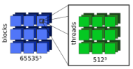
A block may contain up to $1024$ threads, which each execute an instance of the same kernel. Adjacent threads within a block are sub-divided into packages of $32$, each constituting a warp. Each thread may, to first order, be seen to represent a single process on an independent processing unit. There are limits to this picture, however: threads within a single warp are executed at lockstep, i.e. if a single thread enters a code branch, all other threads in the same warp have to wait until it has left the branch again.

All threads within a block may be forced to wait for each other at a particular code segment by the use of an in-built barrier synchronisation function (see Figure 2). This is useful if a code segment relies upon the fact that all threads have terminated the previous segment. All threads within a block share a small region of low-latency shared memory and a set of fast registers. All threads of all blocks share a large region of high-latency global device memory (see Figure 2).

Safe simultaneous write accesses of multiple threads to shared memory resources may be performed using atomic operations. These are in-built routines which prevent ”race” conditions where the read-write cycles of multiple threads are randomly mingled by the hardware, producing an undefined outcome. Trying to synchronize threads belonging to different blocks via atomic operations poses the threat of deadlocks, i.e. that all threads wait for each other to free a particular resource. We observe that this form of global synchronization is most efficiently achieved by exploiting the fact that all threads of a kernel will be synchronized just before the kernel terminates (NVidia 2012d).

The execution of general-purpose GAs on GPUs has shown to be especially efficient using a ”parallel island” model (Pospichal et al. 2010). For the scope of this paper, it is sufficient to notice that this approach by design suffers from data inconsistencies and physically unintuitive selection operators (see Section 3.1), which is acceptable for general optimisation problems, but limits its use within theoretical biology. At the expense of performance, We therefore adapt the model to our needs. We assign one thread to each genome performing the required biological operators. In contrast to (Pospichal et al. 2010), we demand synchronisation between all threads of all block after each generational step in order to preserve data consistency. We also introduce global roulette wheel selection both for sexual and asexual reproduction, instead of the local selection model proposed by (Pospichal et al. 2010).

To this goal, the normalisation constant $N$ is determined using a separate summation kernel (see Figure 4). The roulette wheel selection is then performed from constant device memory which is optimised for memory access patterns that are similar for all threads within the same warp (NVidia 2012d).

True bit-encoding of genome information is significantly more performant than representation by boolean values (Pedemonte et al. 2011). Therefore, we designed efficient bit-wise implementations for mutation, single-point and uniform crossover operators. Importantly, mutation from Poisson distribution proves significantly faster than conventional bit-by-bit flipping in the small µL regime. This means we first randomly choose the number of bits to be flipped and subsequently choose the sites where they should be flipped. The number of bits to be flipped k follows a Poisson process with mean $\lambda$ and probability distribution:

A bitmask is used to avoid multiple flipping at the same sites but may, for $\mu L\ll 1$, be omitted. Figure 5 below demonstrates a significant speed-up even at small genome bytelengths for $\mu L\leq 0.5$. The graph on top corresponds to a genome length of $128$ bytes, the lower graph to a length of $3$ bytes. $105$ iterations using a single CPU thread were performed for each data point. For large genome bytelengths, mutation from distribution is several orders of magnitude faster than bit-wise flipping. For our efficient bit-wise implementations of common evolutionary operators see appendices D, D.1.

We choose to assemble $32$ tile sets per block, scheduling $8$ threads from adjacent warps per assembly. This allows us to store the grid for each assembly within a single shared memory bank, enabling an efficient shared memory access pattern called bank-conflict free access (NVidia 2012b). Ensuring that assembly threads are from different warps allows the usage of atomic operations within each assembly process - atomic operations among threads of the same warps result in undefined behaviour as these threads execute at lockstep (NVidia 2012d). Grid initialisation is performed by all the threads in an assembly process in parallel. This compensates for shared memory access latency.

For the polyomino-assembly fitness function, we a single-threaded movelist-based algorithm offered by Johnston, which stochastically grazes through the assembly frontier on a finite grid of dimension $d$ (Johnston 2010). This implies that $7$ of the $8$ assembly threads are idle during assembly. Each position on the assembly frontier is isotropically checked for ambiguous bonding situations and in this case, the structure is classified nondeterministic. This checks for trivial and first-order steric non-determinism at the same time and we therefore do not distinguish between the two. Higher-order steric non-determinancy is stochastically detected by detailed comparison of k independent assembly processes. See Appendix 2 for a flow chart of the movelist assembly process.

To optimise the assembly process, each bonding label is pre-assigned a list of tiles and their orientations which bond to it. In order to only detect phenotypic nondeterminancy, we remark that this list needs to be further processed in order to eliminate double tile types and symmetric tiles. Also, steric non-determinism detection should be conducted only after the assembly has terminated to allow rotational invariance of assembled shapes - this could be included straightforwardly, but we prefer to be consistent with Johnston et al. 2011.

As shared memory features no heap for dynamic memory allocation, we choose to implement the movelist as a combination of a pre-allocated Last-In-First-Out (LIFO)- stack and grid markings (see below). This implies a higher degree of locality in assembly frontier traversal compared to random traversal using dynamic lists and reduces the need for pre-allocated storage space by about $5$ We, however, observe that the detection of steric non-determinism is not significantly affected by localised traversal as movelist elements are added to the stack in random oder.

Grid-wise comparisons of assembly structures as employed by Johnston are unsuitable for the classification of larger search spaces than $S_{2,8}$ as they are resourceexpensive and ambiguous in higher search spaces (Johnston 2010). As the register manipulation of composite data types in CUDA is tedious, I employ a $32$-bit one-at-a-time hash (Jenkins 1997). Each phenotype shape is hashed by subsequently encoding the positions of all occupied grid sites relative to the coordinates of an assembly grid cropped to the phenotype shape. Cropping is readily parallelisable using atomic operations (see Appendix F.6). For an expected number of $1000$ different phenotypes, the probability that at least one hash collision occurs is

Therefore, a $32$-bit hash is sufficient for the purpose of this paper. We note that hashes may be made rotationally invariant if one chooses to hash each grid for all four orthogonal rotations individually, sorts these hashes by e.g. numerically and sequentially hashes them again with Jenkin’s hash function.

Classifying a genome search space consists of assembling each tile set, hashing the resulting structure and inserting it into a histogram counting the occurrences of each hash. As GPUs have a finite global memory size, on a Tesla $C2050$, only about $2^{1}6$ assembly grids of dimension $19\times 19$ may be stored at any one time. For searchspace classification, this requires execution in batches.

However, the execution may be asynchronous: While the GPU executes one batch, the previous batch is meanwhile sorted on CPU (see Figure 4). For our model, this was shown to efficiently hide CPU processing times. Alternatively, one may just copy the hashes from GPU and the bitstrings for the respective tile sets assembling to those hashes. After having created the histogram on CPU, one may just re-assign assembled structures to hashes by considering the structure which predominantly assembles from the respective tile set.

To verify the correctness of the polyomino assembly routine, I re-classify the search space $S_{2,8}$. Comparing results to Johnston’s yields identical values for the occurrence of deterministic structures (see Figure 8). There is evidence that the mis-classification of non-deterministic structures as deterministic structures can be made arbitrarily small with increasing k (see Figure 8 ). The only phenotype shape with both deterministic and sterically non-deterministic rulesets is found to be the $12$-mer (see Figure 8).

Structures of steric non-determinism outweigh unbound structures by a factor of $\approx 2.2$. This suggests to optimise our assembly algorithm for steric non-determinism detection in the future, which may be achieved by conducting as many assembly processes in parallel at any one time. Finally, a speedup of a factor $2.9$, as compared to Johnston, was detected for our CPU/GPU hybrid implementation.

To demonstrate the flawnessless of our implementation, we implement our genetic algorithm on a test-bed fitness landscape referred to as ‘Fujiyama’-landscape. This landscape consists of a single, broad peak. In evolutionary dynamics, the study of adaptation behaviour on Fujiyama landscapes is insightful as locally, any smooth fitness function may be approximated by a single peak. In simple binary encoding, a suitable fitness function consists of the Hamming weight $H(x)$ of a genome $x$, which is equivalent to the number of set bits in the respective bitstring. We choose to investigate the adaptation and discovery times for a population size of $512$.

Each data point in Figure 10 represents the median of $100$ independent simulations. A simulational cutoff at $20000$ generations is employed. Error bars were derived from bootstrapping with sample size $100$ and $104$ repetitions. I find discovery times to power-law decrease with increasing mutation rate, and the existence of a catastrophic adaptation cut-off in the vicinity of $\mu L=1$. Both these results are fundamental characteristics of genetic algorithms (Johnston 2010). A speed-up of our implementation of factor $7.7$, as compared to Johnston, was measured.

Whereas there exists a large amount of literature on the study of individiual search spaces (Johnston 2010), this is currently not the case for the comparison between different search spaces. Using our CPU/GPU hybrid implementation of JaTAM and a process layout given in Figure 4, we therefore for the first time classify a search space which may be expected to yield phenomenology distinct from $S_{2,8}$. The JaTAM search space for $3$ tile types and $8$ distinct bonding labels is 4096-times larger than $S_{2,8}$ and its classification is expected to yield a rich amount of shape phenomenology.

We provide a GPU classification of the first $32$ bits (thus a $16$th) of this search space, which means that the seed tile type and second tile type may have arbitrary bonding labels, while the third tile type is fixed to bonding labels $\{x_{1},x_{2},y,0\}$, where $x_{1},x_{2}\in[0,7]$ and $y\in\{2,4,6\}$. A frequency classification of deterministic structures shows that the deterministic structures of $S_{2,8}$ are the most frequent ones in $S^{32}_{3,8}$ 8.

This is expected, as the probability that the third tile does not interact with the other two tiles is increased due to the fixed zero bonding site. The frequency differences of certain flipped forms is caused by the fact that these would require tile three to flip bonding labels, which is only possible if $x_{2}=0$ or $y=x_{1}$.

The most frequently encountered structures in $S_{3,8}$ are in fact the simple structures found in $S_{2,8}$. This indicates that simple structures continue to be common in complex ecosystems. Furthermore, the largest structures formed exhibit striking modularity: Most of them consist out of trivially-assembled copies of members of $S_{2,8}$. This motivates the assumption that to first order, $S_{2,8}$ forms the building blocks of $S_{3,8}$. An overview of all $361$ deterministic structures encountered in $S_{3,8}$ can be found in Appendix A.

Langdon advised in 2011 that scientists should refrain from writing new pieces of software using CUDA whenever possible because of the frequent appearance of bugs that were hard or almost impossible to debug (Langdon 2011). As this project featured rather complex kernels (up to 1706 lines for JaTAM classification, which is at least 17- times larger than typical kernel sizes according to Langdon (Langdon 2011)), virtually all of the pitfalls reported by Langdon were encountered. Some of these resulted in intraceable bugs and lead three times to a complete redesign of our source code methodology.

On top of Langdon’s observations, compiler errors generated by the CUDA compiler nvcc were often highly misleading (if it hadn’t crashed during compilation). Tracebacks of cuda-gdb often merely featured unresolved memory addresses and printf functions were prone to buffer overflows, thus making debugging frequently unfeasible and turning the graphics card into an effective ”black box”.

In response, we developed a coding model and compatibility layer that allowed us to first develop and debug our multi-threaded kernel code on CPU. Then, we performed minor modifications to port the code to GPU architecture. This approach in principle also allows easy performance comparisons to implementations on multi-threaded CPUs.

The complexities of code development made it impossible to include some important optimisation features in the current version of our implementation. This may explain why the performance gains achieved for the GA are not as large as may have been expected from the literature (Pospichal et al. 2010). Most notably, our current JaTAM classification spends 83% of its time on assembly grid initialisation. We suggest that this time may be reduced by keeping track of the positions were tiles have been assembled and only re-initialising these. A

Additionally, we found that grid initialisation times could be reduced up to $4$-fold by increasing memory access granularity through the use of pointer re-interpretation (see Appendix D.2). Time spent assembling the structures themselves may be reduced using a parallel assembly process, which may either involve a pure random pick in-place assembly routine (see the flowchart in Appendix 1) or a hybrid approach featuring either separate or shared movelists for each assembly thread (see Appendix F.5 for a push function of a multi-threading safe LIFO stack).

We conclude that even our only modestly optimised GPU implementations yield significant performance gains compared to state-of-the-art CPU implementations. These performance gains may be further increased by performing further optimisation measures as suggested. This indicates that GPUs are likely to have a prominent future in the study of genetic population dynamics.

The difficulties encountered in the development of our GPU implementation immediately raise the question whether it is possible to avoid many common pitfalls by employing state-of-the-art coding standards from within the computer science community. We come up with the following suggestions: Software written in imperative programming languages should be designed from flow-charts (procedural) and/or UML activity diagrams [see App. C] (object-oriented) level. These charts should be supplied for peer-review and enable flow-level analysis.

The source code of unit tests (see Appendix C) and their results should be supplied for peer-review as well to complement flow-level analysis. Domain-specific languages (DSLs) are special-purpose programming languages designed for usage in particular problem domains. Usage of these may abstract away many possible error sources. Creating a new DSL, however, is comparable to writing a compiler and thus difficult and error-prone (Cartney 2012). An example of a system that allows the creation of new DSLs is Cartneys recent work (Cartney 2012). Functional programming languages allow for an abstract flow-independent problem formulation, often resulting in smaller code sizes as well. There exists a large infrastructure of quantitative unit testing tools such as QuickCheck. Equational reasoning allows for fine-grained formal verification in some circumstances (Harper 2012). Problems that are efficiently parallelisable should be expressed in a concurrent programming language.

While a number of concurrent imperative languages are under development, such as python/copperhead (copperhead 2012), functional programming languages arguably embody parallelism more naturally (Chakravarty 2009). The functional programming language Haskell offers industry-grade extensions for data-parallel programming (Wu 2012; GHC 2012). Computer scientists are currently developing functional programming language derivates, such as Accelerate (Chakravarty et al. 2011), which are compiled to CUDA C or Parallel Thread eXecution (NVidia 2007) code and thus produce code for later execution on GPUs.

We conclude that future researchers in the sciences may especially benefit from learning concurrent, as well as functional, programming languages. For performance reasons, we, for this project, chose to program in CUDA C and Python, which are both imperative languages.

References

- Ahnert et al. (2009) Ahnert, S. E., Johnston, I., Fink, M., Doye, J., and Louis, A. Self-assembly, modularity and physical complexity. Phys. Rev. E, 2009.
- Cartney (2012) Cartney, L. Generating GPU code from domain specific languages, February 2012.
- Chakravarty (2009) Chakravarty, M. General purpose GPU computing @ programming languages & systems, 2009. URL http://www.cse.unsw.edu.au/~pls/cuda-workshop09/slides/gpu-research.pdf.
- Chakravarty et al. (2011) Chakravarty, M., Keller, G., Lee, S., McDonell, T., and Grover, V. Accelerating haskell array codes with multicore GPUs. Declarative Aspects of Multicore Programming (DAMP 2011), 2011.
- copperhead (2012) copperhead. copperhead - data parallel python. http://code.google.com/p/copperhead/, 2012. URL http://code.google.com/p/copperhead/.
- Dally (2011) Dally, B. ”Project denver” processor to usher in new era of computing. http://blogs.nvidia.com/2011/01/project-denver-processor-to-usher-in-new-era-of-computing/, January 2011. URL http://blogs.nvidia.com/2011/01/project-denver-processor-to-usher-in-new-era-of-computing/.
- Darwin (2003) Darwin, C. Origin of Species. Signet Classic, 2003.
- Dobzhansky (1973) Dobzhansky, T. Nothing in biology makes sense except in the light of evolution. The American Biology Teacher, 35:125–129, March 1973.
- Domingo et al. (2001) Domingo, E., Holland, J. J., and Biebricher, C. K. Quasispecies and Rna Virus Evolution: Principles and Consequences. R G Landes Co, Georgetown, Tex. : Austin, Tex, March 2001. ISBN 978-1-58706-010-6.
- Doty et al. (2012) Doty, D., Lutz, J. H., Patitz, M. J., Schweller, R. T., Summers, S. M., and Woods, D. The Tile Assembly Model is Intrinsically Universal. pp. 302–310. IEEE Computer Society, October 2012. ISBN 978-1-4673-4383-1. doi: 10.1109/FOCS.2012.76. URL https://www.computer.org/csdl/proceedings-article/focs/2012/4874a302/12OmNyuPKTx. ISSN: 0272-5428.
- Gavrilets (1997) Gavrilets, S. Evolution and speciation on holey adaptive landscapes. Trends in Ecology & Evolution, 12(8):307–312, August 1997. ISSN 0169-5347. doi: 10.1016/S0169-5347(97)01098-7. URL https://www.sciencedirect.com/science/article/pii/S0169534797010987.
- GHC (2012) GHC. Data-Parallel haskell, 2012. URL http://www.haskell.org/haskellwiki/GHC/Data_Parallel_Haskell.
- Group (2012) Group, K. OpenCL - the open standard for parallel programming of heterogeneous systems, March 2012. URL http:/www.khronos.org/opencl/.
- Harper (2012) Harper, T. Interview on software verification, January 2012.
- Hartl & Clark (2007) Hartl, D. and Clark, A. Principles of Population Genetics. Sinauer Associates, Inc. Publishers, Sunderland, MA, 4th edition, 2007. ISBN 978-0-878-93308-2.
- Holland (1992a) Holland, J. Adaptation in natural and artificial systems. MIT press Cambridge, MA, 1992a.
- Holland (1992b) Holland, J. H. Genetic Algorithms. Scientific American, 267(1):66–73, 1992b. ISSN 0036-8733. URL https://www.jstor.org/stable/24939139. Publisher: Scientific American, a division of Nature America, Inc.
- Jenkins (1997) Jenkins, B. Hash functions. 1997.
- Johnston (2010) Johnston, I. Exploration, Exploitation & Complexity in Biological Evolution and Self-Assembly. doctoral thesis, University of Oxford, Oxford, UK, 2010.
- Johnston et al. (2011) Johnston, I., Ahnert, S. E., Louis, A., and Doye, J. Evolutionary dynamics in a simple model of Self-Assembly. Phys. Rev. E, 2011. doi: 10.1103/PhysRevE.83.066105.
- Kumar et al. (2010) Kumar, M., Husian, M., Upreti, N., and Gupta, D. GENETIC ALGORITHM: REVIEW AND APPLICATION. International Journal of Information Technology and Knowledge Management, 2(No. 2):451–454, December 2010.
- Langdon (2011) Langdon, W. Debugging CUDA. GECCO’11, 2011. doi: http://delivery.acm.org/10.1145/2010000/2002028/p415-langdon.pdf.
- Linden et al. (2004) Linden, D., Lohn, J., Hornby, G., and Kraus, W. Evolutionary design of an x-band antenna for NASA’s space technology 5 mission. Antennas and Propagation Society International Symposium, 2004. IEEE, 3:2313 – 2316, 2004.
- M.A.Nowak (2006) M.A.Nowak. Evolutionary Dynamics. 2006.
- Matsumoto & Nishimura (1998) Matsumoto, M. and Nishimura, T. Mersenne twister: A 623-dimensionally equidistributed uniform pseudorandom number generator. ACM Transactions onModeling and Computer Simulation, 8(1):3–30, January 1998.
- Mitchell (1998) Mitchell, M. A Introduction to Genetic Algorithms. The MIT Press, 1998.
- Murthy et al. (2010) Murthy, G. S., Ravishankar, M., Baskaran, M. M., and Sadayappan, P. Optimal loop unrolling for GPGPU programs. In 2010 IEEE International Symposium on Parallel Distributed Processing (IPDPS), pp. 1–11, April 2010. doi: 10.1109/IPDPS.2010.5470423. ISSN: 1530-2075.
- NVidia (2007) NVidia. PTX: parallel thread execution, October 2007. ISA Version 1.1.
- NVidia (2012a) NVidia. Bioinformatics and life sciences (GPU), 2012a. URL http://www.nvidia.com/object/bio_info_life_sciences.html.
- NVidia (2012b) NVidia. CUDA c best practices guide, January 2012b. URL http://developer.download.nvidia.com/compute/DevZone/docs/html/C/doc/CUDA_C_Best_Practices_Guide.pdf.
- NVidia (2012c) NVidia. CUDA toolkit 4.1: CURAND guide, January 2012c. URL http://developer.download.nvidia.com/compute/DevZone/docs/html/CUDALibraries/doc/CURAND_Library.pdf.
- NVidia (2012d) NVidia. CUDA c programming guide, 2012d. URL http://developer.download.nvidia.com/compute/DevZone/docs/html/C/doc/CUDA_C_Programming_Guide.pdf.
- Pedemonte et al. (2011) Pedemonte, M., Alba, E., and Luna, F. Bitwise operations for GPU implementation of genetic algorithms. Proceedings of the 13th annual conference companion on Genetic and evolutionary computation, 2011. doi: 10.1145/2001858.2002031.
- Pospichal et al. (2010) Pospichal, P., Jaros, J., and Schwarz, J. Parallel genetic algorithm on the CUDA architecture. Brno, 2010. Masaryk University. ISBN 978-80-87342-10-7. URL http://www.fit.vutbr.cz/research/view_pub.php?id=9432.
- Ronacher (2012) Ronacher, A. Jinja2, 2012. URL http://jinja.pocoo.org/docs/.
- Rothemund & Winfree (2000) Rothemund, P. and Winfree, E. The program-size of self-assembled squares (extended abstract). 2000.
- Schatz et al. (2007) Schatz, M., Trapnell, C., Delcher, A., and Varshney, A. High-throughput sequence alignment using graphics processing units. BMC Bioinformatics, (8):474, 2007. doi: 10.1186/1471-2105-8-474.
- Schmielau (2012) Schmielau, T. t. Implementing a FIFO-list in shared memory using atomics, 2012. URL https://forums.developer.nvidia.com/t/implementing-a-fifo-list-in-shared-memory-using-atomics-memory-inconsistencies-each-thread-in-a-wa/25864.
- Shannon (1948) Shannon, C. A mathematical theory of communication. Bell System Technical Journal, 27:379–423, 1948.
- Soloveichik & Winfree (2007) Soloveichik, D. and Winfree, E. Complexity of Self-Assembled shapes. SIAM J. Comput., (36):1544–1569, 2007.
- Wagner (2008) Wagner, A. Robustness and evolvability: a paradox resolved. Proceedings. Biological Sciences, 275(1630):91–100, January 2008. ISSN 0962-8452. doi: 10.1098/rspb.2007.1137.
- Wang (1961) Wang, H. Proving theorems by pattern recognition — II. The Bell System Technical Journal, 40(1):1–41, January 1961. ISSN 0005-8580. doi: 10.1002/j.1538-7305.1961.tb03975.x. Conference Name: The Bell System Technical Journal.
- Whitesides & Grzybowski (2002) Whitesides, G. and Grzybowski, B. Self-Assembly at all scales. Science, 295:2418, 2002.
- Winfree et al. (1988) Winfree, E., Liu, F., Wenzler, L., and Seeman, N. Design and Self-Assembly of two-dimensional DNA crystals. Nature, (394):539–544, 1988.
- Wright (1932) Wright, S. The roles of mutation, inbreeding, crossbreeding and selection in evolution. Proceedings of the XI International Congress of Genetics, 8:209–222, 1932.
- Wu (2012) Wu, N. Oxford haskell user group, 2012.
Appendix A Classification of
Appendix B Formalistic treatment of self-assembly
B.1 Winfree’s abstract tile assembly model
Winfree’s model extends planar self-assembly of Wang tiles (Rothemund & Winfree 2000). A Wang tile T is a unit square with edges colored from a binding domain (Wang 1961). The binding domain includes the neutral color null, which does not bond to any other color. A set of symmetric strength functions indicates the interaction strengths between any two colors. Matching colors are assigned some positive integer value interaction strength, all other combinations are set to zero. Tiles may not be rotated nor flipped and there exists an empty tile which does not bond to any other tile. A tileset is the set of all tile types that may be used in the assembly process. Each tile type may be used arbitrarily often. A particular tile occupation pattern of the assembly plane is called a configuration. An individual step in the assembly process consists of randomly adding a further bonding tile from the tileset to the existing configuration. The free energy of a configuration is defined to be the sum over all interaction strengths between the assembled tiles (Rothemund & Winfree 2000). The relative sizes of the free energy of a configuration and an abstract temperature determine whether a given assembly is temperature-stable, i.e. that it is fully connected and will not tend to dissociate into two or more smaller configurations over time. In general, if a tile is added to an existing -stable configuration A, the resulting configuration B is -stable iff the sum over all bonding strengths to neighbour tiles of is greater or equal to (Rothemund & Winfree 2000). In order to fully specify a given assembly process, we need to specify a tile system . Here, T is a tileset including the empty tile and Seed is a set of seed tiles at specified positions, i.e. the initial configuration consists of Seed and empty tiles everywhere else. Each tile system has a map Prod: assembly configurations. The set Term() is the subset of Prod() which includes all configurations that terminate in finite time. If every possible assembly path through Prod() results in an element of Term() in finite time and the cardinality of Term() is finite, then is said to be halting. (Rothemund & Winfree 2000)
B.2 Modifications to Winfree’s aTAM
Due to its two-dimensional nature, it has been suggested that abstract tile assembly model (aTAM) may be used to approximate self-assembly of proteins or protein sub-units on the surface of a planar substrate (Johnston et al. 2011, Fig. 1). In this light, Johnston et al. 2011 have suggested a modified version of aTAM, which I refer to as JaTAM. I now extend Winfree’s aTAM formalism to Johnston’s model. JaTAM fixes to the value of . This makes sense if building block interaction strengths are much larger than thermodynamic noise. The restriction means that for any configuration , is sufficiently large such that is -stable. So can be characterised by a binary matrix . JaTAM fixes to , i.e. colors bond in adjacent pairs, which is in contrast to the color-matching scheme of aTAM. Adjacent pair-bonding may mimick the bonding scheme between complementary DNA bases. This heterogeneous strength function produces different phenomenology from aTAM (Ahnert et al. 2009). Johnston et al. 2011 allow orthogonal rotations of Wang tiles, such that each configuration additionally contains orientation flags of all assembled tiles. Seed is defined to be the first element in the tile set , which is positioned at the center of an empty grid. Two configurations are equivalent iff all assembled tiles at each point of the assembly grid are equivalent in type and orientation. If the positions of all empty tiles coincide between two configurations, then they are shape-equivalent (Johnston 2010). A given is deterministic iff all assembly paths through terminate in equivalent configurations. Otherwise, is non-deterministic. Iff a given configuration contains non-empty tiles at positions outside an origin-centred square of dimension , then is said to be unbounded by . Otherwise, is bounded by . Iff is halting, then we can always find a finite, positive such that is bounded by . Let the assembly frontier be the set of all assembly grid positions that are occupied by an empty tile and have at least one non-empty neighbour tile. Let’s choose some non-deterministic . For any configuration , let denote the set of configurations generated after one further tile has been assembled on the assembly frontier of . Let be the point where tile has been assembled. If contains a subset of configurations which correspond to equal but are not all equivalent to each other, then is said to exhibit trivial non-determinism. Steric non-determinism arises if at least two partial assembly paths exclude each other without the involvement of trivial non-determinism. Phenomenologically, this arises when two or more independently growing ”arms” converge (Johnston 2010). may exhibit trivial non-determinism and steric non-determinism at the same time. I now proceed by extending Johnston’s terminology by defining a shape-similarity measure. I define the shape-difference of two configurations to be the number of non-coinciding empty tile positions between and . Then, iff are just bounded by , the shape-similarity of is defined to be equivalent to . As tile-shaped building blocks may bind to a substrate from either above or below, and Johnston et al. 2011 suggest a future assembly-system, which allows tiles bonding from two sides to be arbitrarily flipped in the substrate plane. In this paper, however, I will restrict myself to JaTAM, which is reasonable if we assume that tiles only bind to the substrate from a single side.
B.3 Encoding genome information
By Shannon (Shannon 1948), in order to label genome microstates, an average number of bits are needed. While, in principle, we are free to choose any such encoding, there are particular choices of binary encodings that are more natural than others based on characteristics of the evolutionary operators acting on the search space . These characteristics should be equivalent to their counterparts in natural DNA encoding.
Applying a suitable mutation operator to some genome needs to yield another element . A formal way of stating this is to say that is closed under the operator . Furthermore, any must be transformable into any arbitrary element with non-zero probability in a finite number of steps, i.e. is permuting. A suitable single-point crossover operator needs to be such that is closed under it as well. However, it is not a permuting operator, which can be seen by choosing two genomes with uniform base occupations - however often we recombine the two, we will never be able to create a permutation that contains the third or fourth base type used by DNA encoding. A characteristic property of is, however, that it preserves the relative order of all genes involved.
I conclude that with respect to mutation, the choice of what bases constitute a particular gene is arbitrary. For single-point crossover, however, relative order of genes has to be preserved and this can in the general case only be defined if all bases belonging to a particular gene sit at adjacent locations in the genome. The observation of genetic drift, however, strongly depends on the correlation between a particular gene and its phenototypic expression. Whether it is possible to define a gene-interpretation for Johnston’s model that allows for strong correlations between genotypes and phenotypes is a key question for further research. Kolmogorov complexity is defined as the shortest program size written in a language which can output a bitstring . We will in the following define to be the language of a Universal Turing Machine. A phenotype shape in aTAM can be defined by supplying a list of the locations of all non-empty tiles, which I call a list representation of that shape. Winfree et al. 1988 showed that of the list representation of a scale-free phenotype shape is proportional to the minimum number of tile types, with respect to some tile system , that deterministically assembles that shape (Soloveichik & Winfree 2007). Even though the relationship to of heterogeneous strength functions is not strictly proven (Soloveichik & Winfree 2007), Ahnert et al. 2009 provide an algorithm which computes n with respect to a phenotype shape assembled by JaTAM and is of the same order as the respective Kolmogorov complexity(Ahnert et al. 2009). With respect to JaTAM, I conclude that a strongly phenotype-correlated gene-interpretation might consist of gene being the minimum number of tile types required to compute the phenotype shape encoded in the genome and a gene which encodes a notion of shapescale. Such an encoding does not exclude a constant bitstring binary encoding with respect to . Defining the action of the operator on such a binary encoding, however, is non-trivial and subject to further research.
I finally describe the constant bitstring binary encoding used by Johnston et al. 2011 and how the respective action of may be defined. Johnston encodes a general tile set in the genome by sequentially encoding each tile in the tile set to a bitstring, starting with the seed tile. This is achieved by subsequently encoding all four colors of the tile in the order north-east-southwest, as looking down on the configuration grid. The number of bits required to encode a particular color is and Johnston always minimises the number of bits required. The action of on this representation of is to flip a number of distinct bits, where is Poisson-distributed with mean . As this implies a non-zero probability for the flipping of just a single bit, sequential -operations can be used to traverse arbitrary Hamming weight distances in search space and is thus permuting. To achieve closure under , I conclude that Johnston’s encoding restricts to integer powers of . It is now trivial to define the map tileset, which decodes Johnston’s binary encoding into a tileset.
Appendix C On Flow Charts, Unit Tests and UML diagrams
In many situations, flow charts are an insightful way to represent the procedural large-scale flow of a program. In order to turn a piece of code into a flow chart, one first represents all branches and loops as an empty flow-chart and then fills in the pictograms with some short-hand summary of the action of the underlying code. The content of each pictogram then defines a particular code unit. The functionality of each code unit may be described by the help of abstract pseudo code. In order to ensure the integrity of a code unit, a carefully-written unit test should be designed. A unit test defines a set of input values to a code unit and specifies the desired set of output values. The distribution of input values can be a random distribution or taylored to test particularly suspicious parameter ranges. The assertion strength of a unit test is thus dependent on the choice of input values. A principal advantage of unit tests is that they can act on black boxes, i.e. program parts whose precise internals that cannot or should not be presented to a general audience. By publishing the input parameters of the unit test, however, and the resulting output parameters, one can display code integrity without the need of detailed code disclosure or analysis. Furthermore, large and complex code units may be broken down into simpler, independent components which can be unit-tested individually. If a piece of software is designed in an object-oriented way, flow charts may be replaced by Unified-Modeling language (UML) diagrams. UML is a very broad standard allowing the graphical representation of flow processes in a large number of domains. A particular type of UML diagram is a class diagram which represents all classes, their attributes and their relationships with each other. There exist tools that can generate UML class diagrams from source code and also some that allow the generation of source code from such a diagram.
C.1 Tournament Selection in Haskell
In order to illustrate how functional programming is independent of program flow, I attach snippets in C and Haskell used for tournament selection: We supply a list of weights and a cut-off index (which is usually chosen randomly) and would like our function to return the counter index of the element where the sum of the weights is greater or equal to the cut-off index.
C.1.1 C-implementation
We initialise global parameters as follows:
C.1.2 Haskell-implementation
The parameters should be initialised as follows:
We note that tourn is simply a curried, recursive function. The internal flow of this function is determined by the compiler only.
Appendix D Efficient bit-wise implementations of common evolutionary operators
D.1 Mutation from Poisson Distribution
An implementation of mutation from Poisson distribution follows below. Note that we could reduce the required storage space for the bitmask, of course at the expense increasing computing time, by using a dynamic list to keep track of the flipped bits. Dynamic lists in shared memory, however cannot be efficiently implemented as there is no heap available.
D.2 Single-point crossover
An efficient implementation of single-point crossover, which uses byte-wise operations instead of bit-wise operations. A further performance gain would be achieved by further increasing the granularity using reinterpret_cast as the genome bytelength exceeds a couple of bytes (up to for double precision).
D.3 Uniform crossover
An efficient implementation of uniform crossover, where both genomes are randomly interleaved on bit-level. Note that interleaving occurs in multiples of bytes, which is the number of bytes that a call to the random number function generates.
Appendix E PyCUDA - tips and tricks
This section includes some work-arounds which I needed to employ in order to get things work and which I could not find in any forum or document.
E.1 Getting curand to work
PyCUDA is designed such that python code can call kernel functions defined in C/C++. For this purpose, it requires knowledge of the exact reference name of the function used by the compiler. In C, this is merely the name of the function as defined by the programmer. C++, however, supports functions of equal naming but different namespaces. In order to keep track of these functions, the compiler name-mangles them to some label unpredictable to PyCUDA. As curand_kernel-header uses different namespaces, it requires name-mangling to be activated, while the rest of the kernel code may not feature it. This problem may be solved by setting the Source Module-Option ‘no_extern_c’ to ‘True’ and enclosing everything but the header in extern ‘C’-brackets.
E.2 Unrolling for-loops using meta-templating
Interestingly, unrolling small for-loops may result in performance gains of up to a factor of 2, as has been observed previously (Murthy et al. 2010). An automatised way of unrolling loops at runtime is the usage of a metatemplating language, such as Jinja2(Ronacher 2012). The following code segment demonstrates the -times unrolling of a loop:
Appendix F Selected Algorithms
F.1 Bit operations and casting
Using genome bit-representation instead of e.g. boolean representation allows the usage of very fast bit-operations which directly translate into x processor instructions. For reference, I include basic usage of bit operations on the nth bit in C/C++:
Bit setting
Bit clearing
Bit testing
Bit toggling
Modulo 2 operations
All these operations can be effectively parallelised for a larger number of bits using bitmasks.
F.2 The use of reinterpret_cast
The data type of a memory segment may be re-interpreted as a different data type by the usage of either unions in C and / or reinterpret_cast in C++. With caution, pointers reinterpreted by reinterpret_cast may be de-referenced. In this way, char-arrays may be initialised with a step length of up to -byte on GPU, which I found to be about times faster than char-wise initialisation. For gcc-based compilers (such as likely nvcc), dereferencing a reinterpreted pointer may trigger the following warning: warning: type punned pointer will break strict-aliasing rules. This warning can be eliminated by setting the flag -fno-strict-aliasing. This does take away some optimisation options from the compiler, however, from my experience is usually acceptable performance-wise.
F.3 Bit operations and casting in Python
As python does not natively implement fixed-size numeric datatypes, the usage of bit operations may not be as performant as for C/C++. However, equivalent operators may be used e.g. for calculating Jenkin’s hash (Jenkins 1997). The size of the data type may then be selected aftwards using a bitmask (i.e. to select a -bit data type from a pythonic number x, we may use x&=0xffffffff to set higher bits to zero.) As python does not offer pointer manipulation natively, one needs to employ a foreign-function interface such as ctypes in order to implement C/C++-style union data types and/or type casting.
F.4 One-at-a-time Hash
The following is an efficient implementation of a 32-bit hash function taking one byte at a time by Jenkins (Jenkins 1997). This so called One-at-a-time hash has a decent avalanche behaviour and is very fast.
F.5 Reentrant LIFO-Stack
I thank tera (Schmielau 2012) for making me aware of undercurrent and overcurrent detection issues arising from the use of atomic operations in CUDA with unsigned data types. The following is a push-function, designed by tera, which has been made multi-threading safe for use in a multi-threaded LIFO-stack implementation:
Note: pos_p should be initialised to . Note also that changes in the usage of atomic functions which would be valid for boost threads may readily lead to data inconsistencies for usage with CUDA.
F.6 Parallelised grid cropping
The following parallelised code determines the upper left and the lower right crop corner of an assembly grid:
![[Uncaptioned image]](2205.15311v1/simplified_movelist_flow_chart.png)
![[Uncaptioned image]](2205.15311v1/detailed_movelist_flow_chart.png)
Appendix G Determination of the maximally required movelist size
![[Uncaptioned image]](2205.15311v1/movelist_equiv_unjoined.png)
Joining two open ends is movelist-size-wise equivalent to leaving them unjoined.
![[Uncaptioned image]](2205.15311v1/max_movelist.png)
Left: A growth pattern suspected to have maximum movelist occupation for LIFO-stacks. Right: A growth pattern with maximum movelist occupation for dynamic lists. The black tile is the seed tile. Note that the spiral on the right has kinks, while the structure on the left has one less - this explains why the spiral is expected to have a smaller maximum movelist than then the left-hand side.