Predictive Rate Selection for Ultra-Reliable Communication using Statistical Radio Maps
Abstract
This paper proposes exploiting the spatial correlation of wireless channel statistics beyond the conventional received signal strength maps by constructing statistical radio maps to predict any relevant channel statistics to assist communications. Specifically, from stored channel samples acquired by previous users in the network, we use Gaussian processes (GPs) to estimate quantiles of the channel distribution at a new position using a non-parametric model. This prior information is then used to select the transmission rate for some target level of reliability. The approach is tested with synthetic data, simulated from urban micro-cell environments, highlighting how the proposed solution helps to reduce the training estimation phase, which is especially attractive for the tight latency constraints inherent to ultra-reliable low-latency (URLLC) deployments.
Index Terms:
Radio maps, ultra-reliable low-latency communication, Gaussian processes, statistical learningI Introduction
Ultra-reliable low-latency communications (URLLC) is one of the most significant novelties brought by 5G, aiming to support wireless connections with very stringent requirements in terms of latency and reliability. From a physical layer viewpoint, the inherent randomness of wireless channels is the major challenge, rendering a fundamentally unreliable communication link. In cellular systems, instantaneous channel state information (CSI) estimation is widely used to adapt the resource allocation and transmission rate to the actual channel state, requiring an estimation phase before the data transmission. However, when looking towards URLLC, two main drawbacks arise: i) it introduces a latency that may be unacceptable for mission-critical applications; and ii) in the ultra-reliable regime, assuming the channel stays exactly constant during both estimation and transmission phases may be wrong [1], depending on the actual channel dynamics.
As an alternative, the communication parameters can be chosen according to statistical knowledge of the channel, based on parametric or non-parametric models, so that a reliability constraint is met with given confidence [2]. While parametric models can be fitted using relatively few samples, the models widely used in wireless communications, particularly Rayleigh or Rician, are not intended for URLLC [3]. Models based on, e.g., extreme value theory, can be better suited for URLLC, but they can also be challenging to apply in practice as they rely on results that are valid only asymptotically [4]. At the other extreme are non-parametric models, which palliate the issue of model mismatch but require a massive number of samples that is prohibitive in most realistic situations, especially for non-stationary environments [2].
Reducing the required number of samples to obtain statistical knowledge of the channel is therefore vital for URLLC. One promising option is to exploit the spatial correlation of the channel, e.g., by using radio maps [5, 6, 7, 8, 9]. These maps usually model the average signal-to-noise ratio (SNR) across space using methods such as Kriging interpolation [6, 7] and Gaussian processes (GPs) [8] and have been applied for, e.g., resource allocation [5], positioning [8], and route planning [9]. However, because the maps considered in these works focus on the average SNR, they provide limited information about the channel distribution required for URLLC (unless a parametric model is assumed, such as Rayleigh fading).
Modeling the SNR beyond its average is usually avoided in radio maps as the spatial correlation of fast fading decorrelates within a few wavelengths. However, the spatial independence of fast fading only applies to the instantaneous values and not its long-term statistics. In fact, it is reasonable to expect that the long-term statistics vary smoothly in space due to shared dominant paths, scatterers, etc. Thus, channel samples collected from other users in the network can, when combined with location information, be expected to be good predictors of the channel statistics beyond the average at a new location. Motivated by this, in this paper, we propose a novel approach of using statistical radio maps to estimate the outage capacity in a wireless network. The resulting map is used to select the transmission rate for a new user joining the system, such that a specific reliability constraint can be met with high probability without the need for the device to collect any channel samples, thereby reducing the overall latency. A central feature of the proposed map is that it includes a parameter to control the trade-off between model uncertainty and transmission rate.
II System model and problem definition
II-A Signal Model
We consider a URLLC scenario comprising a single base station (BS) serving several user equipments (UEs) within an area11 1 The method can be applied without modifications in any finite-dimensional real space, but we focus on for clarity and assume that the UEs are located at the same height. . The BS and the UEs communicate both in the uplink and downlink, and the packets must be delivered with high reliability and low latency to the receiver, which precludes the possibility of estimating the instantaneous channel prior to transmission. To ease the presentation, we will assume that the transmitted signals are received without interference, but we stress that this assumption is not required as long as the distribution of the interference power is stationary. Following this, a signal of length transmitted either by the BS to a UE or by a UE to the BS is received as
| (1) |
Here, is the complex channel gain (comprising both fast and slow fading) drawn from some unknown distribution conditioned on the location of the UE and some parameter characterizing the environment. Specifically, is common to all UEs and captures all propagation parameters within the cell, such as the location of blockages and scatterers, providing the spatial consistency and correlation to . Finally, denotes the additive white Gaussian noise with elements drawn independently from , where is the power spectral density and is the bandwidth. The transmitted signal is assumed to be normalized, i.e., , so that the instantaneous SNR of the signal is
| (2) |
The SNR is conditionally independent given and across both time and users. However, the environment, characterized by , will remain fixed, so we will denote the distribution of the SNR simply as for each location . Under this model, the error probability of a packet transmitted with a given rate is dominated by the event of outage [10], which is given by the probability that the instantaneous rate supported by the channel is less than , i.e.,
| (3) |
where is the cumulative distribution function (CDF) of given .
II-B Problem Definition
We consider the general problem of selecting the maximum rate for a user at any given location within the cell while ensuring that the outage probability in (3) stays below some . Under the assumption that the distribution of is perfectly known, this translates to selecting the rate equal to the -outage capacity
| (4) |
where is the -quantile of . However, in our case — or in any realistic case — where the distribution of the SNR is unknown and needs to be estimated, the defined -outage capacity is not meaningful, and the rate selection problem becomes less trivial.
To assist the rate selection, we assume that the BS has collected SNR measurements over some period from previous users in the network and stores a dataset comprising a set of independent SNR measurements from locations for . It is assumed that the user locations and propagation environment (i.e., ) are stationary throughout the scenario so that for each user, the SNR is only affected by multipath fading characterized by . Furthermore, the user locations are assumed to be perfectly known — see [11] for an analysis of how localization error can affect the reliability in scenarios like the one modeled here.
We here seek to learn a function , where is the family of rate selection functions that predict the rate for any location based on the observations . In stark contrast to previous uses of radio maps, we aim to account for the uncertainty of SNR estimation in the rate selection function. To that end, and inspired by the concept of probably correct reliability (PCR) introduced in [2], we formulate the rate selection as the following optimization problem:
| (5a) | ||||
| s.t. | (5b) | |||
Constraint (5b), denoted meta-probability , accounts for the uncertainty in the prediction due to the data , and thus controls how much weight the system should give to model uncertainties when selecting the rate. We can observe that even though solving (5) would render a rate meeting the reliability constraint, computing (5b) is infeasible unless the channel and data distributions — namely and the distribution of the sampling process — are perfectly known. Hence, in the following sections, we provide an approximate solution to the rate selection problem based on the statistical radio maps generated from and the associated uncertainty.
III Rate Selection using Statistical Radio Map
This section presents the framework to solve the objective defined in (5) by modeling and predicting the spatial behavior of the channel gain using statistical radio maps. The framework is divided into three phases. First, we use the dataset to obtain a non-parametric estimate of the -quantile of the SNR. Then, we construct a statistical radio map that models the spatial behavior of the quantile using a Gaussian process, which provides an inherent way to capture the uncertainty in the predictions. Finally, the radio map is used to predict the rate at new locations using an estimated meta-probability that elegantly considers the model’s uncertainty. Note that although we focus here on the quantile prediction, a similar approach can be used to construct a radio map that characterizes any statistic that may assist the communication.
III-A Non-parametric quantile estimation
We adopt a non-parametric estimator to estimate the quantile SNR at each location in the dataset. This contrasts with the typical approach of assuming a parametric fading distribution, e.g., Rayleigh/Rician or Nakagami fading, and then estimating the distribution parameters using e.g., maximum likelihood optimization. However, while parametric distributions typically require few samples to estimate, they are susceptible to model mismatch, which may result in prediction errors greater than what can be tolerated in URLLC [2].
Therefore, for each entry in the available dataset , we first estimate the -quantile of the logarithmic-scale SNR as [12]
| (6) |
where is the -th order statistics of and is the floor function. This generates a new dataset with the estimated -quantile at observed locations on the radio map. Note that the estimate in (6) is unbiased and admits an asymptotic Gaussian distribution as [12, p. 356]. Notably, the quantile estimate does not require knowledge of the underlying distribution of the SNR and can be used as input for spatial prediction. The main disadvantage compared to parametric estimates, on the other hand, is the excessive number of samples required for estimation when is low. In fact, (6) shows that scales inversely with , and is only well defined when . However, the SNR samples used to estimate the quantiles as input to the GP can be collected over a long period.
III-B Spatial interpolation with Gaussian processes
We proceed to model the spatial variation of the estimated -quantiles across the cell area , which will allow us to predict the quantile at a new location that is not contained in . To this end, we first normalize the quantiles as
| (7) |
where and are the sample mean and standard deviation of , respectively. Following the result that order statistic based quantile estimates are asymptotic Gaussian [12], we assume the observation model , where is an independent Gaussian random variable with zero mean and variance . Additionally, it is assumed that is a Gaussian process [13], where at any finite subset of locations is jointly Gaussian such that
| (8) |
Here, the mean vector is defined in terms of the mean function for , parameterized by . The elements of the covariance matrix are given by , where is a symmetric kernel function parameterized by . In the context of radio channels, the absolute exponential kernel
| (9) |
with parameters , is referred to as the Gudmundson correlation model [14], and has been widely applied along with a log-distance mean function to model how the average SNR varies across space [6, 7]. Note that is the variance of the Gaussian process and is the correlation distance, which tends to be in the order of the size of blocking objects when modeling shadow fading [15]. Through numerical experimentation, we found that the Gudmundson correlation model is also well suited to model the -quantile of the SNR which is therefore adopted to characterize the spatial correlation of . For the mean, we use , as commonly done in the literature [13].
The radio map is constructed for a regular grid of locations simultaneously, denoted . In order to predict the Gaussian process at locations , we express the joint distribution of the noisy observations and quantiles in the grid as
| (10) |
where is the identity matrix. Following (10), the predictive distribution for where is also a multivariate Gaussian distribution with [13]
| (11) | ||||
| (12) |
Equations (11) and (12) constitute the predictive distribution for and are referred to as the predictive mean and covariance, respectively. Because the model produces a full distribution of the predicted quantiles, it allows us to capture the uncertainty of the estimates, which we will make use of in the rate selection in the next subsection.
Finally, we note that so far we have assumed that the hyperparameter is fixed. However, in practice it needs to be estimated as well. We do this using maximum likelihood estimation by numerically maximizing the likelihood of the observed data with respect to . We gently refer the reader to [13, Ch. 5] for further details on the procedure.
III-C Rate selection function
Once the statistical radio map is generated at the BS and broadcasted to new UEs joining the system at location , the predictive distribution of the quantile can be used to select the rate. Specifically, we aim to use the statistical information about to solve (5). Note that we assume to be known.
As discussed in Sec. II-B, the difficulty of computing the meta-probability in (5b) is the requirement of perfect knowledge of both channel and data distributions, which is unfeasible in any realistic setup. To circumvent this, we replace this knowledge by the predictive distribution of the quantile from the statistical map, rendering an approximated solution to (5). From (3) and (5b), we can write
| (13) |
where is the SNR at location . Denoting as the CDF of , we have
| (14) |
which is directly given by the CDF of the true SNR quantile (in logarithmic scale), i.e.,
| (15) |
Since is unknown, we replace it by the predictive distribution obtained from the statistical radio map, from which we have the normalized quantile , with and as in (11) and (12). Then, we denormalize the quantile by isolating from (7), leading to with and , where and are the global mean and standard deviation obtained from the dataset as defined in Sec. III-B. Hence, given the meta-probability constraint , an approximate solution to (5) fulfills
| (16) |
whose solution follows as
| (17) |
where is the inverse error function. Note that the meta-probability only matches the target confidence when the modeling assumptions for quantile estimation and spatial correlation are correct. Nevertheless, provides a way to control how conservative the selected rate should be. The entire procedure (map generation and rate selection) is summarized in Algorithm 1.
IV Numerical evaluation
For numerical evaluation, we consider UEs in the area m with the BS in the middle at m. The dataset is composed of locations (unless otherwise stated), each containing independent SNR observations. To imitate a realistic clustered setup, the locations are sampled from a modified Thomas process [16]. We first simulate a continuous Thomas process in the area (to remove edge effects) with a parent process rate of , a daughter process rate of , and a standard deviation of . Points outside are discarded, and the remaining points are rounded to the nearest two meters and then randomly and independently thinned until unique points remain.
The channel coefficients used to compute the SNRs in (2) across the region are simulated with the simulation tool QuaDRiGa using the 3GPP NR Urban Micro-Cell scenario with line of sight (see [17, p. 81]) with BS height m, UE height m, transmit power of dBm, and GHz as central frequency. Since QuaDRiGa is a geometric channel simulator, we emulate independent fast fading by adding uniformly distributed random phase shifts on top of each path arriving to the receiver, and then adding up the contributions of all the paths to obtain a narrowband channel coefficient. With the resulting channel gains, the SNR values are calculated as in (2) with KHz and noise power dBm. To evaluate the predicted outage probabilities, we also simulate test data comprising SNR values at locations forming a uniform grid with m spacing.
We start by comparing the predictive means of the -quantile of obtained for a sample dataset using Algorithm 1 to the quantiles estimated from in Fig. 1. The left map shows obtained from , while the right map shows the quantile predicted from the radio map, i.e., for each calculated using the procedure in Sec. III. It can be seen that the predictive mean is generally close to the test values except for areas far away from any observed location, e.g., in the right part of the map. However, the predictive variance (which is not depicted) is also significantly higher in these areas as well.

We now turn our attention to the rate selection problem, where we aim to predict the maximum rate for the unobserved locations on the map satisfying an outage probability of at most (we refer to this as predictive rate selection). Unless otherwise stated, we set . For comparison, we use a baseline scheme, which simply selects the rate based on measurements from the closest observed location. Specifically, if is the closest observed location to the target location , then the baseline scheme chooses the rate as
. The outage probabilities resulting from the rate selection schemes are empirically computed using the test data — see Fig. 2 for an example based on the same scenario as in Fig. 1. The figure shows that the outage probabilities obtained using the predictive rate selection rarely exceed the target , whereas the baseline scheme often exceeds the target outage probability.

The results in Figs. 1 and 2 clearly depend on the spatial distribution of the user locations. For example, the predictive rate selection scheme is generally very conservative in areas with no observations (due to higher predictive variance), leading to an outage probability several orders of magnitude below the target. On the other hand, the baseline scheme is generally close to the target outage probability only for points close to an observed location. To analyze the performance with less dependency on the particular realization of the UE locations in , we repeat the rate selection process in Algorithm 1 with the same SNR quantiles as shown top left in Fig. 3, but for different realizations of the UE location sampling process. We then estimate the meta-probabilities defined in (13) by counting the number of times the resulting outage probability exceeds at each location, as seen in the top right and lower plots in Fig. 3. We see that the meta-probabilities of the baseline scheme are often above , which means that the outage probability exceeds for more than half of the simulations at those locations. The predictive scheme, on the other hand, is typically below the target outage probability. Interestingly, we see a strong negative correlation between areas with high meta-probability and areas where the -quantile of the SNR is lower than its surroundings. For example, the predictive rate selection has a high meta-probability close to the BS in the center, where the quantile is about dB lower than its immediate surroundings. Intuitively, this makes sense since predictions made from around the BS, where the quantile is high, will predict a similarly high quantile, which will cause a high outage probability. A reverse effect is seen for areas with a higher quantile than its surroundings, where the outage is below the target with high probability.
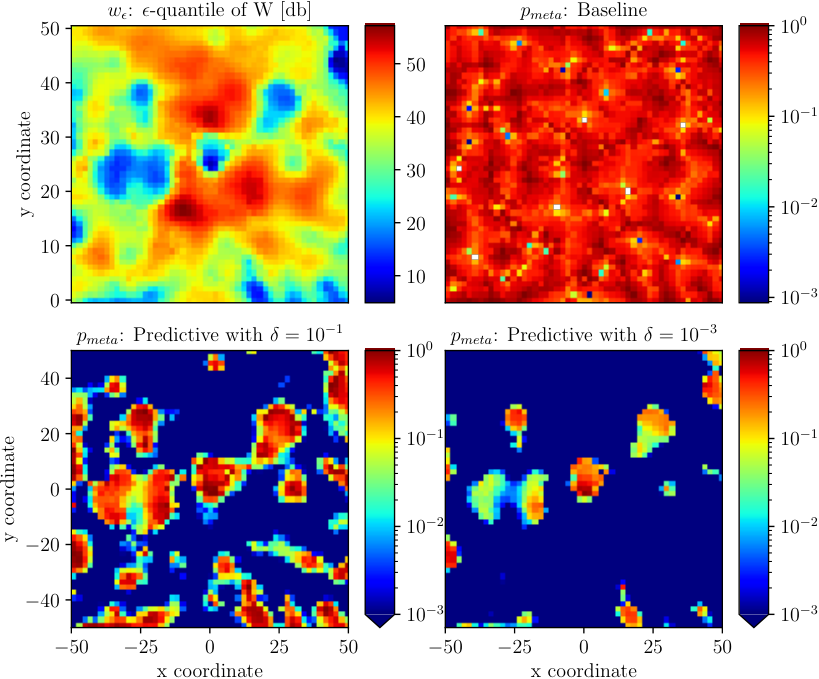
Fig. 4 shows the empirical CDF of the outage probabilities obtained across all locations on the map and realizations of the UE locations in . The figure also shows the distribution of outage probabilities for two new scenarios, namely when rate selection is based only on observations from locations, and when the UE locations in are drawn according to a binomial point process, i.e., uniformly from .
Similarly to the previous results, we observe that the outage probabilities are generally lower for the predictive rate selection than the baseline. The probabilities at correspond to , and we see that the predictive rate selection slightly exceeds the target meta-probability of in the three scenarios, which is due to modeling mismatches. However, it is significantly closer to the target than the baseline scheme. The meta-probability is closer to the target reliability in the scenario with the binomial point process than the clustered process, which is expected since the test locations are also located uniformly across the map. Furthermore, the outage probability for predictive rate selection has a high probability not only of being below the target of but also of being below or even lower, which reflects the high cost of being uncertain about the channel statistics.
To evaluate this aspect, we define the throughput resulting from rate as the average rate when the system is not in outage [2], i.e.,
| (18) |
where is the indicator function. To account for spatial variation of the SNR, we compute the normalized throughput, denoted , by dividing with the throughput of the -outage capacity from (4) such that
| (19) |
Note that from this definition, a value means that the rate is greater than the -outage capacity, and thus the target reliability constraint is not satisfied. Fig. 5 shows the distribution of the normalized throughput resulting from the considered rate selection methods. It can be seen that the throughput for the predictive rate selection in far most cases is smaller than one, meaning that the reliability constraint is satisfied. This is in contrast to the baseline scheme, which in many cases does not meet the target reliability. Furthermore, although the throughput of the predictive rate selection is conservative, it is generally far from zero, suggesting that the proposed method is suitable for rate selection in the URLLC regime.
V Conclusion
In this paper, we have considered the problem of rate selection for URLLC when the channel statistics are unknown. To circumvent the problem of having to collect a very large number of samples for non-parametric channel estimation, we have proposed a framework that unites the ideas of radio maps and statistical learning. In particular, our framework uses a GP radio map to model the distribution of the -outage capacity across space, allowing us to predict the outage capacity at unseen locations using non-parametric quantile estimates obtained from only a few locations. Using the predicted distribution, we introduced a rate selection rule inspired by the concept of meta-probabilities from statistical learning, which controls how prediction uncertainty penalizes the rate. Through numerical results, we demonstrated that the proposed framework can accurately model the outage capacity and that the rate selection rule satisfies the reliability target with significantly higher probability than a baseline scheme, confirming that the framework is suitable for URLLC. Future work will include extensions such as the ability to handle non-stationary propagation environments, modeling of localization uncertainty, and reducing the number of measurements required at each location.
References
- [1] V. N. Swamy, P. Rigge, G. Ranade, B. Nikolić, and A. Sahai, “Wireless channel dynamics and robustness for ultra-reliable low-latency communications,” IEEE J. Sel. Areas Commun., vol. 37, no. 4, pp. 705–720, 2019.
- [2] M. Angjelichinoski, K. F. Trillingsgaard, and P. Popovski, “A statistical learning approach to ultra-reliable low latency communication,” IEEE Trans. Commun., vol. 67, no. 7, pp. 5153–5166, 2019.
- [3] P. C. F. Eggers, M. Angjelichinoski, and P. Popovski, “Wireless channel modeling perspectives for ultra-reliable communications,” IEEE Trans. Wireless Commun., vol. 18, no. 4, pp. 2229–2243, 2019.
- [4] N. Mehrnia and S. Coleri, “Wireless channel modeling based on extreme value theory for ultra-reliable communications,” IEEE Trans. Wireless Commun., vol. 21, no. 2, pp. 1064–1076, 2022.
- [5] H. Abou-zeid, H. S. Hassanein, and S. Valentin, “Optimal predictive resource allocation: Exploiting mobility patterns and radio maps,” in IEEE Global Commun. Conf. (GLOBECOM), 2013, pp. 4877–4882.
- [6] V.-P. Chowdappa, C. Botella, J. J. Samper-Zapater, and R. J. Martinez, “Distributed radio map reconstruction for 5g automotive,” IEEE Intell. Transp. Syst. Mag., vol. 10, no. 2, pp. 36–49, 2018, conference Name: IEEE Intelligent Transportation Systems Magazine.
- [7] K. Sato, K. Suto, K. Inage, K. Adachi, and T. Fujii, “Space-frequency-interpolated radio map,” IEEE Trans. Veh. Technol., vol. 70, no. 1, pp. 714–725, 2021.
- [8] X. Wang, X. Wang, S. Mao, J. Zhang, S. C. G. Periaswamy, and J. Patton, “Indoor radio map construction and localization with deep Gaussian processes,” IEEE Internet Things J., vol. 7, no. 11, pp. 11 238–11 249, 2020.
- [9] X. Mu, Y. Liu, L. Guo, J. Lin, and R. Schober, “Intelligent reflecting surface enhanced indoor robot path planning: A radio map-based approach,” IEEE Trans. Wireless Commun., vol. 20, no. 7, pp. 4732–4747, 2021.
- [10] W. Yang, G. Durisi, T. Koch, and Y. Polyanskiy, “Quasi-static multiple-antenna fading channels at finite blocklength,” IEEE Transactions on Information Theory, vol. 60, no. 7, pp. 4232–4265, 2014.
- [11] T. Kallehauge, P. Ramírez-Espinosa, K. Kansanen, H. Wymeersch, and P. Popovski, “A primer on the statistical relation between wireless ultra-reliability and location estimation,” IEEE Wireless Commun. Lett., 2022.
- [12] A. Stuart and O. J. Keith, Kendall’s Advanced Theory of Statistics: Distribution Theory, 6th ed., ser. Kendall’s Library of Statistics. Halsted Press and Wiley & Sons, New York, 1994, vol. 1.
- [13] C. E. R. Rasmussen and C. K. I. Williams, Gaussian Processes for Machine Learning. The MIT Press, 2006.
- [14] M. Gudmundson, “Correlation model for shadow fading in mobile radio systems,” Electronics Letters, vol. 27, no. 03, 1991.
- [15] A. Goldsmith, Wireless Communications. Cambridge University Press, 2005.
- [16] J. Moller and R. P. Waagepetersen, Statistical inference and simulation for spatial point processes. CRC Press, 2003.
- [17] Quasi Deterministic Radio Channel Generator User Manual and Documentation, v2.4.0 ed., Fraunhofer Heinrich Hertz Institute, October 2020.