Mountain formation by repeated, inhomogeneous crustal failure in a neutron star2022Mountain formation by repeated, inhomogeneous crustal failure in a neutron star–APPENDIX E: MOMENT OF INERTIA CALCULATION
Abstract
The elastic crust of a neutron star fractures repeatedly as it spins down electromagnetically. An idealised, macroscopic model of inhomogeneous crustal failure is presented based on a cellular automaton with nearest-neighbour tectonic interactions involving strain redistribution and thermal dissipation. Predictions are made of the size and waiting-time distributions of failure events, as well as the rate of failure as the star spins down. The last failure event typically occurs when the star spins down to of its birth frequency with implications for rotational glitch activity. Neutron stars are commonly suggested as sources of continuous gravitational waves. The output of the automaton is converted into predictions of the star’s mass ellipticity and gravitational wave strain as functions of its age, with implications for future observations with instruments such as the Laser Interferometer Gravitational Wave Observatory (LIGO), the Virgo interferometer, or the Kamioka Gravitational Wave Detector (KAGRA).
Keywords:
asteroseismology – gravitational waves – stars: evolution – stars: neutron – stars: rotation1 Introduction
Mountains form on neutron stars through various thermoelastic and magnetic forces (Ushomirsky et al. 2000a; Payne & Melatos 2004; Haskell et al. 2008; Mastrano & Melatos 2012; Gittins et al. 2021). They break the star’s axisymmetry and lead to the continuous emission of gravitational waves at levels potentially approaching the sensitivity of instruments like the Laser Interferometer Gravitational Wave Observatory (LIGO), the Virgo interferometer or the Kamioka Gravitational Wave Detector (KAGRA). (Riles 2013; Woan et al. 2018; Reed et al. 2021). Several recent LIGO-Virgo-KAGRA searches have placed increasingly stringent constraints on the mass ellipticity of neutron star mountains (Abbott et al. 2019a; Abbott et al. 2019b; Abbott et al. 2019c; Abbott et al. 2019d; Abbott et al. 2019e; Abbott et al. 2020; Papa et al. 2020), and more sensitive searches are planned in the near future. More broadly, mechanical failure in response to crustal deformation (Baym & Pines 1971; Pines & Shaham 1972) has been invoked in the context of numerous transient astrophysical phenomena such as rotational glitches in pulsars (Ruderman 1976; Middleditch et al. 2006), soft gamma-ray repeaters (Kaplan et al. 2001; Hurley et al. 2005; Baiko & Chugunov 2018) and fast radio bursts (Suvorov & Kokkotas 2019). The connection between crustal deformation, mechanical failure, and the above phenomena remains a matter of debate. Viable alternatives exist, e.g. superfluid vortex avalanches in the context of pulsar glitches (Anderson & Itoh 1975; Warszawski & Melatos 2011). Predictive, falsifiable models are needed to discriminate between the alternatives, based either on the microphysics (Andersson et al. 2012; Piekarewicz et al. 2014) or on the long-term size and waiting-time statistics of the transients (Fulgenzi et al. 2017; Melatos et al. 2018; Carlin & Melatos 2020).
The far-from-equilibrium tectonic process by which mountains form on macroscopic scales is currently unknown (Caplan & Horowitz 2017; Gittins et al. 2021). To date modelling has concentrated on calculating the microphysics of crust failure (Horowitz & Hughto 2008; Horowitz & Kadau 2009; Chugunov & Horowitz 2010; Horowitz et al. 2011; Baiko & Chugunov 2018). Molecular dynamics simulations of ions responding to a slowly ramping, quasistatic stress indicate that the crust fails globally (above a strain of ) rather than fracturing locally into cracks due to the high pressure (Horowitz & Kadau 2009). Some modelling has treated the whole star on macroscopic scales as it evolves through a quasistatic sequence of elastic and hydromagnetic equilibria. Giliberti et al. 2019 and Giliberti et al. 2020 studied two-layer and continuously stratified models respectively and evaluated the effect of the adiabatic index and stellar mass on the build up of mechanical strain in the crust. However, the latter papers describe slow, reversible evolution on the spin-down time-scale. They do not include the stick-slip dynamics of repeated failure and healing, which involve a mixture of short and long time-scales and lead to irreversible, history-dependent outcomes, i.e. hysteresis (Jensen 1998; Sornette 2006).
In this paper we address the problem of mountain formation by repeated crustal failure on macroscopic scales driven by spin down. The paper is structured in the following way. Section 2 deals with how the crust deforms secularly due to spin down and the redistribution of stress and dissipation of energy in response to failure, which leads to radial movement. A cellular automaton is constructed to capture the dynamics of repeated failure. Section 3 presents the long-term statistics of failure events generated by the automaton. Section 4 calculates the ellipticity and hence gravitational wave strain as a function of the star’s age. The calculations in this paper do not include magnetic fields for simplicity. Complementary studies of plate tectonics involving the interplay between superfluid neutron vortices and magnetic flux tubes are presented by Ruderman 1991a; Ruderman 1991b; Ruderman 1991c; see also Srinivasan et al. 1990.
2 Tectonics
A neutron star loses angular momentum over its lifetime due to processes such as magnetic dipole radiation and gravitational wave emission (Lyne et al. 2014). As the balance of gravitational and centrifugal forces changes, so does the shape of the star (Pines & Shaham 1972). A neutron star is primarily composed of an incompressible superfluid interior and a solid crystalline crust (Horowitz et al. 2011; Fattoyev et al. 2018; Baiko & Chugunov 2018; Chugunov 2020; Kozhberov & Yakovlev 2020; Kozhberov 2020). The superfluid interior adjusts to spin-down deformation, but the crust, being an almost-rigid solid, does not deform as easily. Mechanical strain builds up in the crust up to and beyond the point of failure.
We propose that the accumulated strain causes sections of the crust to fail when the breaking strain is exceeded locally (Franco et al. 2000; Fattoyev et al. 2018). The failed sections move radially, creating a mountain locally as well as dissipating energy and redistributing strain to neighbouring sections, which may then fail themselves in response. These knock-on dynamics are modelled by a cellular automaton described in Section 2.6.
2.1 Secular crustal deformation without failure
In the absence of failure, we consider a biaxial star, which is axisymmetric and rotating about the -axis. The star is composed of a fluid core and solid, almost-rigid crust, whose principal moments of inertia vary quasistatically on the spin-down time-scale, which is much longer than the rotation period relevant in gravitational wave applications, for example.
The slow, secular deformation of the star is calculated using the formalism outlined by Franco et al. 2000. Briefly, this approach starts by equating the sum of the gravitational and centrifugal forces to the elastic forces and considers a Lagrangian perturbation to that equilibrium. To summarise the main result, when the star spins down an infinitesimal amount, , from some angular velocity, , to a smaller value, , an infinitesimal volume element at moves to , where is the deformation vector. Its components are given below in spherical coordinates,
| (1) | |||||
| (2) | |||||
| (3) |
where is the second Legendre polynomial with argument . The coefficients satisfy the simultaneous equations,
| (4) | |||||
| (5) | |||||
| (6) | |||||
| (7) |
In Eqs. (4)–(7), and are the total and core radii of the non-rotating configuration respectively. We also define as the surface Keplerian velocity, and as the transverse speed of sound, where is the shear modulus, is the crustal density, and is simply the part of Eq. (1) that depends on ; is its derivative. In this paper we set km, km, kms-1, kms-1 and assume a 1.4 solar mass star (Franco et al. 2000; Fattoyev et al. 2018). These are illustrative values for intrinsically uncertain quantities; the goal of the paper is to introduce the idea of tectonic activity modelled by a cellular automaton, not to make precise quantitative predictions. The boundary conditions, Eqs. (4)-(7), come from requiring that there are no shear forces at the crust-core and crust-vacuum boundaries and that the star is in mechanical equilibrium at those same boundaries.
The strain tensor,
| (8) |
defines the strain angle, , at every point in the crust as the difference between its largest and smallest eigenvalues. Landau & Lifshitz 1970 discussed in detail the connection between and . The latter quantity, , is the increase in the total strain angle, , at a particular location as a result of spinning down infinitesimally from to , not the current strain angle that has built up over the entire course of spin down, i.e. from to . In this paper we mostly refer to the strain angle (fractional deformation), rather than stress (force per unit area). However the two are linearly related up until the point of failure (Horowitz & Hughto 2008; Horowitz & Kadau 2009).
In Fig. 1 we plot contours of the strain angle in the crust based on the model of Franco et al. 2000. It is apparent that the strain angle is highest at the crust-core boundary at the equator. This property influences how the strain angle is evaluated in the automaton in Section 2.6. In this model is constant throughout the crust for simplicity, but there are other models where this is not the case. For example in the papers by Giliberti et al. 2019 and Giliberti et al. 2020, which include mass stratification, the maximum strain occurs at the poles, the base of the crust, or the stellar surface, depending on the exact model. Likewise Cutler et al. 2003 found that the stress is greatest at the crust-core boundary yet the strain is greatest at the stellar surface, because increases with depth.
2.2 Microphysics of failure of the crystal lattice
Simulations of the crustal material have been performed in the past, mostly focusing on the microphysics of the crustal lattice (Horowitz & Hughto 2008; Horowitz & Kadau 2009; Horowitz et al. 2011; Caplan & Horowitz 2017; Baiko & Chugunov 2018). In particular Horowitz & Kadau 2009 found an exceptionally strong crust with breaking strain . They also found that the crust fails abruptly and universally, without cracking locally, because the pressure suppresses the formation of local imperfections, such as voids and dislocations. Such imperfections typically form in terrestrial materials and cause localised failure. The above breaking strain is much larger than previous estimates, e.g. (Smoluchowski 1970), which assume lower densities and do not use a long-range Yukawa-type interaction.
The results of Horowitz & Kadau 2009 are for cubic femtometres of material. In a real star it is likely that the macroscopic crust undergoes a different mode of failure than the microscopic material because of the presence of lattice dislocations, grain boundaries, vestiges of previous failures, and other mesoscopic im-perfections (Kittel et al. 1996). Even though the pressure is high, it is unlikely realistically to iron out these non-equilibrium features completely, and their existence seeds the production of additional imperfections, as the star spins down.
2.3 Macroscopic redistribution and dissipation of stress due to failure
In this section, we present an idealised model for how the strain angle accumulated during spin down as in Section 2.1 is dissipated and redistributed macroscopically following a failure event triggered microscopically as in Section 2.2.
Failure on macroscopic scales is a discrete process in general. In this model we break up the crust into a two-dimensional grid of cells and track the strain angle in each cell. When the strain angle exceeds a critical threshold (i.e. when the cell fails) we dissipate and redistribute energy stored in the cell as mechanical potential energy. A given cell labelled with indices and ( with coordinates occupies the volume defined by , , . This defines a lattice of “rings” of cells evenly spaced along the -axis with each “ring” containing cells evenly spaced in . In Fig. 2 we display top-down and side-on diagrams of the cell volumes, in the upper and lower panels respectively. The black dots are the coordinates assigned to each cell. One can see that the cells are similar in shape to trapezoidal prisms with radial thickness . They are defined to encase the fluid core with no overlap at all times. More details, including an explanation of how overlap is prevented, are given in Appendix A. The deformation vector of a cell and associated strain angle are determined as per Section 2.1 and evaluated at . We evaluate and at the crust-core boundary, because that is where the crust is densest and stiffest and where most of the elastic energy is located.
Each cell is assigned a random breaking strain in the range informed by the polycrystalline stress-strain curve calculated by Horowitz & Kadau 2009. Following Fattoyev et al. 2018 we define failure to occur when is satisfied for some , i.e. failure occurs when the strain angle in some cell exceeds its breaking strain. Other valid definitions of failure include the Tresca criterion, for some , as used by giliberti2021starquakes in the context of accreting neutron stars. We use the terms strain and strain angle interchangeably for simplicity’s sake.
| Energy Component | Formula |
|---|---|
| Elastic energy in failed | |
| cell before failure | |
| Elastic energy in failed | |
| cell after failure | |
| Energy distributed from failed | |
| cell to neighbours | |
| Plastic work to raise failed cell | |
| Increase in gravitational potential | |
| energy of failed cell | |
| Decrease in gravitational potential | |
| energy of lowered neighbours | |
| Heat dissipated during plastic work | |
| to raise failed cells | |
| Heat dissipated after | |
| lowering of neighbours | |
| Total heat dissipated | |
| Total energy received by | |
| cell from failed neighbours | |


The elastic potential energy in a material of volume under strain is given by the strain-energy formula
| (9) |
When a volume of material fails it partially relaxes. A portion of stays within the failed volume, while the rest does reversible mechanical work on neighbouring volumes, or does plastic work on the failed volume. Table 1 summarizes for the reader’s convenience the key energy components which are stored, redistributed, and dissipated in and around a failed cell before, during, and after failure. We refer repeatedly to the formulas and notation in Table 1 throughout the rest of the paper.
A failed cell retains some fraction, , of its energy after failure. This means that it retains some fraction of its strain as per
| (10) |
In this paper is constant and takes the same value in every cell. When a volume of material fails the neighbouring material experiences an increase in strain in general, i.e. redistribution. The failed volume becomes less able to support mechanical loads, shifting the load onto the neighbouring material by doing reversible, mechanical work (R. Hertzberg & Hertberg 2013). Accordingly adjacent cells receive some reversible fraction, , of the energy surrendered by the failed cell, , defined in the third row of Table 1 in terms of parameter . In this paper is constant and takes the same value in every cell. Each adjacent cell receives an equal portion, . 11 1 The cells closest to the poles have three neighbours rather than four. If one of these cells fails, energy is redistributed to cells and for or to cells and for . Additionally cells with and are adjacent. This also modifies the formula in the last row of Table 1. The strain of adjacent cells increases according to
| (11) | |||||
| (12) |
where is the total energy distributed to cell by all of its failed neighbours.
The elastic energy decrement left over after redistribution to adjacent cells, namely , goes into deforming the crust outwards against the force of gravity. The deformation is plastic and irreversible. In order to preserve hydrostatic equilibrium, the crust surrounding the failed cell must simultaneously move radially inwards such that the gravitational potential energy of the whole crust does not change; that is, the average radius of the entire crust does not change. The potential energy lost, when the crust moves inward through the centrifugal-gravitational potential, is dissipated as heat. A recipe for moving the crust inward and outward and calculating the plastic work done is presented in Section 2.4.
2.4 Radial movement
In response to the post-failure relaxation process described in Eqs. (10), (11), and (12), the failed cell moves outwards radially according to,
| (13) |
with defined below in Eq. (16). Its nearest neighbours move inward radially according to
| (14) |
with and and defined below in Eq. (17). The angular coordinates of each cell are held constant. is calculated by determining the elastic potential energy difference between the pre- and post-failure states of the crust (i.e. the first minus the second and third rows in Table 1) and moving the failed cell the corresponding radial distance through the gravitational-centrifugal potential of the star. The total potential is given by (Franco et al. 2000)
| (15) |
where is the gravitational constant, is the density of the fluid core, and is the eccentricity of the ellipse defined by the meridional cross-section of the star. We calculate from
| (16) |
where is the shear modulus of crust at the crust-core boundary as calculated by Lander et al. 2015, who used the methodology of Horowitz & Hughto 2008, and the factor describes thermal losses during plastic deformation as discussed in Section 2.5 (fiducial value ).
As explained above, in order to preserve hydrostatic equilibrium, the cells adjacent to the failed cell must move inward such that the gravitational-centrifugal potential energy of the whole crust remains constant. Assuming for simplicity that the potential energy change is equal for every adjacent cell,22 2 As described in Footnote 1 the cells closest to the poles have three neighbours rather than four. If one of these cells fails their neighbours move inwards per Eq. (17) but a factor of should be used rather than the factor of on the left-hand side of the equation. we obtain
| (17) |
for the four cells and . In other words the crust bends such that the centrifugal-gravitational potential energy of the whole crust is constant. The radius of the crust does not rise or fall on average.
The statement that the failed and adjacent cells move outward and inward respectively is consistent with Eq. (15), because the gravitational-centrifugal potential increases strictly with . Fig. 3 illustrates how neighbouring cells lift or fall by different heights and produce an uneven solid surface. The crust is supported after lifting by a combination of fluid pressure from below and shear forces from adjacent regions of the crust.
When a cell fails its breaking strain resets in the above range, . The microscopic change of the crystal structure after experiencing failure is still a matter of investigation (Baiko & Chugunov 2018; Chugunov 2020; Kozhberov 2020) and we do not investigate it here. We assume that the crystal structure relaxes to a similar pre-failure configuration (albeit under a different strain) on a timescale much shorter than the waiting time until the next failure.

2.5 Thermal losses during plastic deformation
When a body undergoes plastic deformation a fraction, , of the plastic work done on the body is converted into heat. The right-hand side of Eq. (16) gives the reversible energy transfer i.e. the energy not lost as heat during plastic deformation. Replacing the factor with gives the energy that is lost as heat. Together with the heat released by the neighbouring cells moving inward, the total heat dissipated by crustal movement (triggered by failed cells) in a particular time-step is denoted by in what follows. It is obtained by summing row four (equivalent to row nine) in Table 1 over all cells that fail in the time-step.
The exact value of depends on the specific material in question and a variety of factors such as strain, strain rate and deformation history (Rittel 1999; Rosakis et al. 2000; Macdougall 2000; Hodowany et al. 2000; Ravichandran et al. 2002). Appendix B outlines briefly some of the key issues. It is challenging to predict from first principles even for terrestrial materials, where one is guided by controlled experiments, let alone for neutron star matter. Common terrestrial metals like copper and steel are measured to have , reflecting a competition between internal friction and the formation of lattice defects. In the face of this uncertainty, we adopt in this paper, taking the conservative position astrophysically that most of the elastic energy released during plastic deformation is dissipated as heat and does not contribute to mountain formation. Hence the mass ellipticity and gravitational wave signal (which are proportional roughly to ) are smaller than one would predict otherwise. The reader is encouraged to experiment with other values. We reiterate that we neglect magnetic forces in this paper, in order to focus on the new idea of tectonic activity modelled by a cellular automaton. Hence the energy lost during plastic deformation is due to internal friction and vibrations, not due to rearranging the magnetic field (Srinivasan et al. 1990; Ruderman 1991a; Ruderman 1991b; Ruderman 1991c).
2.6 Cellular automaton
We now combine the idealised tectonic physics of deformation and failure in Sections 2.1, 2.3, 2.4 and 2.5 into a simple automaton, which is iterated to study the long-term, far-from-equilibrium dynamics of the system. The state of each cell of the automaton is described by five numbers, , which are updated at each time-step. Here the and indices refer to the cell index and corresponds to the time-step.
The automaton is initialised as a Maclaurin spheroid with eccentricity , a representative value. The oblateness at birth is uncertain, with estimates reaching as high as . (Haensel et al. 2002). For at birth and before failure we have (Franco et al. 2000; Haskell et al. 2008)
| (18) | |||||
| (19) | |||||
| (20) |
The cellular automaton entails the following steps:
- 1)
Choose and .
- 2)
- 3)
Assign to each cell a random breaking strain and .
- 4)
- 5)
Calculate and for each cell. Set .
- 6)
If cell has it undergoes failure.
- 7)
Decrease by , where is constant throughout the simulation.
- 8)
Repeat from step (4) until drops to .
We assume that the star spins down in response to a magnetic dipole torque satisfying , and hence
| (21) |
with
| (22) |
Given and we can calculate the age of the star from its current angular velocity. In this paper we assume that the time-scale of failure events is much shorter than the spin-down time-scale; failure is effectively instantaneous.
In this paper we simulate a star with the following fiducial parameters: km, km, kgm-3 (Haensel et al. 2002; Chamel & Haensel 2008), kgm-3, , Hz, Hzs-1, and therefore s. For these values the ratio is in line with typical pulsars. Again, the values above are illustrative only; their uncertainties are outweighed by uncertainties in other material properties, such as , , and . For and the above fiducial values Eq. (16) implies mm for a failure event at on the equator.
3 Failure event statistics
Starquakes triggered by failure events have been suggested as important factors driving the phenomena of glitches (Ruderman 1976; Franco et al. 2000; Middleditch et al. 2006; Chugunov & Horowitz 2010; Fattoyev et al. 2018; Giliberti et al. 2020; Bransgrove et al. 2020) and gamma-ray bursts (Kaplan et al. 2001; Hurley et al. 2005; Horowitz & Hughto 2008). Recent theoretical work also shows that the long-term statistics of avalanche processes in neutron stars, including starquakes, can be understood in terms of well-defined stochastic mechanisms describing stress accumulation and release, e.g. state-dependent Poisson processes (Melatos et al. 2008; Warszawski & Melatos 2013; Fulgenzi et al. 2017; Carlin & Melatos 2019a; Carlin & Melatos 2019b) and Brownian threshold processes (Carlin & Melatos 2020). Models of these mechanisms make specific, falsifiable predictions about the long-term probability distribution functions (PDFs) and cross- and autocorrrelations of event sizes and waiting times and are therefore a promising tool for distinguishing between classes of microphysical processes, including crustal failure in the starquake context (Fulgenzi et al. 2017; Melatos et al. 2018; Carlin & Melatos 2019a; Carlin & Melatos 2019b; Carlin & Melatos 2020). We are therefore motivated to investigate the statistics of failure events in this paper, partly as input into the foregoing studies.
We define a failure event as occurring at a particular time-step, when one or more individual cells fail during that time-step. Our definition is therefore expressed collectively for simplicity: for the purposes of terminology, a time-step corresponds to either zero or one global failure events, no matter how many individual cells fail, and whether or not the failed cells are contiguous (i.e. single or multiple disjoint avalanches). The size of a failure event (, measured in units of joules) is defined as described in the first paragraph of Section 2.5. The waiting time (, measured in units of ) is the time between one event and the next.
This section is structured as follows. In Section 3.1 we present representative examples of the size and waiting-time distributions and comment on their general form. In Section 3.2 we calculate size and waiting time cross-correlations, which may offer interesting opportunities to falsify crust failure models observationally. Section 3.3 explores how the distribution of failure events depends on the redistribution and dissipation parameters and . The values of and also control the long-term level of tectonic activity in the star, which is studied in Section 3.4.
3.1 Size and waiting-time distributions


We start by presenting the PDFs of the event sizes and waiting times for representative values of the failure parameters, . They are displayed in Fig. 4. The PDFs are qualitatively similar across the relevant domain of and (see Section 3.4). The waiting-time PDF (upper panel of Fig. 4) rises steeply at low and has an approximately power-law tail at high . The peak occurs at in units of . However a reasonable number of failures occur with shorter and longer () waiting times. The size PDF (lower panel of Fig. 4) is more tightly peaked, reaching a maximum at J with a full-width-at-half-maximum of approximately J.
We observe that the waiting-time PDF is approximately a power law with a cut-off at low . The cut-off is an artefact of how time is discretised in the automaton: is fixed and therefore sets a minimum time increment and hence a minimum . The power-law distribution is evidence of a non-Poissonian point process governing failure events, consistent with other self-organized critical systems (Jensen 1998). The reader is referred to Appendix C for further details.
Regarding the size PDF, the size of an event depends, in part, on the volume of the failed cells. This affects the location of the cut-off at low . In the lower panel of Fig. 4 the cut-off in is . For and a cell at the equator failing at , we have J from Table 1, in good agreement with the observed cut off. In contrast, the largest events correspond to avalanches involving large numbers of cells. Their sizes are unaffected by the total number and volume of cells in the automaton. With the peak in the size PDF occurring at J, the most common events involve cells.
Different events have different sizes due to the random breaking strains, , and the random number of cells failing during one time-step, . It is interesting to check how much each of these two factors affects the dispersion of event sizes, where “dispersion” here is a general term for the characteristic width of the size PDF, which does not necessarily equal exactly the full-width-half-maximum or standard deviation. The failure energy, , depends quadratically on , which is randomly assigned to each cell as per Section 2.6. Comparing the mean of the square and the square of the mean of the , and distributions, we obtain , and for . This implies that the distribution is, in relative terms, approximately as broad as the distribution and broader than the distribution. Hence the stochasticity of avalanches (i.e. ) explains somewhat more of the dispersion in event sizes than the random breaking strains of individual cells.
We find that the number of events is linearly proportional to the number of cells in the automaton, and is inversely proportional to the number of cells, but the observable, macroscopic work lost as heat () is unaffected by the grid size or the frequency decrement. The volume of the crust that undergoes failure also converges with and . Appendix D investigates the convergence of the automaton.
3.2 Size-waiting-time correlations
In Fig. 5 we plot vs for individual events. Events cluster within ranges of with tails in . The central value of in each cluster depends on and . We find strong evidence for a correlation between and with the direction and strength of the correlation dependent on the value of but less sensitive to . For we find a Spearman rank coefficient of with a p-value . At the Spearman rank coefficient is with p-value , and at the Spearman rank coefficient is with p-value . The Spearman rank coefficients are calculated with data from five realisations of the automaton, with approximately 400 events per realisation per value of .
The positive correlation at large is due to the secular deformation of the crust. Spin-down deformation moves the crust away from the equator and towards the poles (see Fig. 15 in Appendix A, alternatively see Fig. 2 in Franco et al. 2000), causing the equatorial cells to grow as the star ages. Events later in the star’s life are larger on average because the equatorial cells, where strain is greatest, have greater volume. Additionally strain accumulates slower, as the star ages, causing waiting times to be longer when the star is older. Later failures tend to be larger due to the larger equatorial cells, and have longer waiting times because the star is older, hence the positive correlation between event size and waiting time for large . However for small later events are smaller than earlier ones: a cell failing at late times finds most of its neighbours have already failed, are strained below and so are unlikely to be part of an avalanche. Later events being smaller than early events leads to a negative correlation between event size and waiting time. Equatorial cell volumes can increase by a factor of due to spin-down deformation, but a failed cell has up to four neighbours that may be part of an avalanche (and neighbours have neighbours). Hence the magnitude of the correlation is greater for small than for large . Furthermore, by examining Fig. 7 in Section 3.3, we see that heat is dissipated quickly for small but takes longer for large . Large events are disfavoured at late times for small but not for large .
Some events per run ( of all events) have long waiting times . These occur late in the star’s life , when the star is spinning at Hz), when the strain build up has slowed considerably. These events are left out of Fig. 5 for clarity but are included in the calculation of the Spearman rank coefficients.
3.3 History of activity and energy release


In previous sections we consider the size of events, where the size of an event is defined as the total heat dissipated by all failed cells, contiguous or not, in the time-step of the event. We are also interested in the total heat dissipated by all events up to an arbitrary instant in the star’s life, i.e. the total energy released since birth, by failure, from the crust and dissipated as heat. The heat dissipated from crustal failure is relevant to a variety of astrophysical mechanisms that may connect to crustal failure such as glitches (Pines & Shaham 1972; Ruderman 1976) or fast radio bursts (Suvorov & Kokkotas 2019).
It has been suggested that some energetic transient phenomena such as gamma-ray bursts (Kaplan et al. 2001; Hurley et al. 2005; Horowitz & Hughto 2008) originate in the breaking crust of neutron stars. In this and similar contexts, it is interesting to ask how much mechanical potential energy is stored in the crust and how much of the total energy deposited into the crust is released as heat. In the upper panel of Fig. 6 we display the total mechanical potential energy stored in the crust at time for a variety of values of . In the middle panel we display the cumulative energy dissipated as heat () in all failure events up to time . In the lower panel we display the fraction of energy deposited into the crust that is dissipated as heat, i.e. the data of the middle panel divided by the black line of the upper panel. For the fiducial parameters listed at the end of Section 2.6 approximately J are deposited into the crust in the form of elastic potential energy over the star’s life and between J and J of heat are dissipated in all failure events. Between and of the deposited energy is eventually lost as heat depending on and . The star releases the most heat near and the least near . The qualitative behaviour over time is consistent across parameter space but quantitative variations are significant, as explained in Section 3.4.
The fraction of heat dissipated over time does not vary much with but does vary with . In Fig. 7 the fractional heat dissipated by time is approximately given by , an arbitrary empirical fit. Tectonic activity persists longer, when is higher, because cell relaxation is less complete and a failed cell is more likely to fail for a second time, dissipating additional heat later in the star’s life. Most tectonic activity occurs early in the star’s life, with of the heat dissipated from to depending on . This corresponds to a rotation frequency from to . The star remains seismically active even after losing the majority of its rotational energy, because the strain since birth is stored in the crust in a metastable, far-from-equilibrium configuration, which relaxes via repeated failure on a time-scale longer than . The run-to-run dispersion in energy released as a fraction of total energy released is small and is consistent across parameter space, with .
Failure is a time-limited process; beyond a certain age, the star spins down sufficiently that the crust does not fail in any location during the remainder of its life. It is therefore meaningful to speak of the ultimate volumetric fraction of the crust that ever undergoes failure. The ultimate volumetric failure fraction is plotted versus and in Fig. 8. The total volume of the crust that fails reaches a minimum near with of the crust failing and a maximum near with of the crust failing, where above means the same regions of the crust fail repeatedly. The volumetric failure fraction increases with because stronger nearest-neighbour interactions lead to larger avalanches. However the dependence on is not as straightforward. Cell relaxation is less complete, when is higher, through Eq. (10), which makes secondary failures more likely. On the other hand, the nearest-neighbour interaction is weaker, when is higher, which produces smaller avalanches. The effects in the previous two sentences counteract each other. If is small the nearest-neighbour interaction is always weak so the effect of on avalanche size is irrelevant.
For and the corresponding energy density of failure is Jm-3. When of the crust fails the total heat released while moving the crust is J. This is consistent with the results in Fig. 9 in which we display the total heat dissipated in all failure events for a variety of values of .


3.4 Redistribution and dissipation
The dissipation and redistribution of strain in the crust, governed by the parameters and respectively, have a significant impact on the quantitative outcomes of failure. In this section we examine the impact of the values of and on the volume of the crust that undergoes failure, the and PDFs, and the total heat dissipated while moving the crust in failure events.
In Section 3.1 we examine the PDFs of and for the representative values . Now we turn to examining the effects of different values of and on the PDFs. In Fig. 10 the PDFs for a range of values of and are presented. Most immediately we can see that changing or has little to no effect on the PDF. This insensitivity to the parameters is because events are driven by the build up of strain due to spin down which is unaffected by or . In contrast, the effects on the PDF, presented in Fig. 11, are notable, with a shift in the locations of the peaks of approximately one order of magnitude from to . Events are smaller for larger and . The dispersion of the PDF increases with . Near the sizes are spread over approximately two orders of magnitude; near the sizes are spread over three orders of magnitude. The nearest-neighbour interaction is stronger with higher so avalanches are more common and larger and the dispersion is larger too.
Let us now return to , the total heat dissipated by failure. Fig. 9 yields a maximum J and a minimum J. Unlike the volumetric failure fraction the total heat dissipated is strictly decreasing with and . Larger and mean that events are smaller. Additionally, whereas the volumetric failure fraction is more sensitive to than to , the reverse is true for ; it is more sensitive to than to . As increases decreases significantly. Individual failed cells are less energetic and the nearest-neighbour interaction is also weaker. Not only are individual events smaller but avalanches are smaller and less frequent; both effects work to decrease . Conversely increasing strengthens the nearest-neighbour interaction causing avalanches to be larger and more frequent but individual cell failures to be less energetic; these effects partially counteract one another.


4 Mass Ellipticity
As well as the statistics of failure events, we are also interested in the local mountains that failure events create. These mountains break axisymmetry, creating a non-zero ellipticity leading to continuous emission of gravitational waves which may be detectable by modern instruments such as LIGO-Virgo-KAGRA (Riles 2013; Woan et al. 2018). There have been several searches for continuous gravitational wave signals (Abbott et al. 2019a; Abbott et al. 2019b; Abbott et al. 2019c; Abbott et al. 2019d; Abbott et al. 2019e; Abbott et al. 2020; Papa et al. 2020), but none have been found to date.
In this section the physical quantities of interest are the star’s ellipticity and gravitational wave strain. These quantities are numerically convergent as a function of the angular velocity decrement, , and the number of cells ; see Appendix D for further details.
4.1 Definition
The moments of inertia of the star are necessary to calculate its ellipticity, , and thus the characteristic wave strain, , of the gravitational wave signal. The moment of inertia tensor, , is defined as
| (23) |
In Eq. (23) is the number of mass elements in the system, is the mass of the element, is the distance to the mass element from the origin (the centre of the star in this case) and is the coordinate of the mass element ().
Local failure affects the moments of inertia of the star unequally, which breaks axisymmetry and leads to . In order to calculate the moments of inertia of the whole star we need the masses and centres of mass of each crustal cell and of the fluid core. The calculations of the foregoing quantities are detailed in Appendix E. As at the end of Section 2.6 we assume that the crust and core are of uniform density, with kgm-3 (Horowitz et al. 2007), and kgm-3 and the crust is 1 km thick, i.e. km. These fiducial values are selected for the sake of illustration; an exhaustive study of the parameter space is postponed to future work.
The off-diagonal moments of inertia are much smaller than the other moments of inertia; typically we find . The principal moments of inertia are well approximated by , , and . The ellipticity of interest for gravitational wave applications is given by
| (24) |
As the star is triaxial, there is a second ellipticity in the problem, namely . This is dominated by the centrifugal bulge, which is axisymmetric and therefore does not emit gravitational waves. We therefore concentrate on in what follows.


4.2 Ellipticity evolution
The long-term evolution of determines directly the long-term evolution of a tectonically active neutron star as a gravitational wave source. In Fig. 12 we plot the ellipticity versus time for and . The differences between simulations of the same parameters are purely stochastic. The behaviour of is qualitatively similar across parameter space.
We obtain until the first failure at then increases steeply. The behaviour is stochastic; individual events may increase or decrease but over the long term increases. As the rate of change of strain is independent of or , the first failure always occurs at nearly the same time with small variations coming from . Fast spin down early in the star’s life causes many failures, hence the fast rise in . At late times failures happen less frequently and approaches a final value.
The standard deviation in is comparable to its mean, with across parameter space, compared with the total heat dissipated, where we find . This is because the locations of the failed cells, among other factors, determine the size and sign of the change in . Suppose the first cell to fail is located at , i.e. lying directly on the -axis. As a result of this cell failing increases but does not33 3 Strictly does change due to the movement of the neighbouring cells, but the change is negligible for the purpose of this illustrative example.. The first failure always increases because it breaks axisymmetry, but subsequent failures are not guaranteed to increase . A second failure located at , i.e. on the -axis, increases but not , causing to decrease. However if instead the second failure is located at , i.e. on the negative -axis, increases further. Failure events increase or decrease by various amounts depending on where the failed cells are located relative to previous failures. The change in also depends on factors such as the size of and the number of cells that fail, but the spatial location of failures is the most significant source of dispersion.
In Fig. 13 we present the final ellipticity of the star, as it varies with and . The average final varies between and across parameter space. However the dispersion is large and individual simulations can achieve ellipticities over . It is apparent the final ellipticity of the star is insensitive to and . As is increased, becomes smaller, through Eq. (16), and the nearest-neighbour interaction becomes stronger. Cells move less upon failure, causing to decrease, but more cells fail, causing to increase. These two effects counteract one another meaning a weak net effect on . As is increased, becomes smaller and the nearest-neighbour interaction becomes weaker, both of which cause to decrease. But larger allows cells to fail multiple times causing to increase. Again these effects counteract one another meaning a weak net effect on .
Although the final ellipticity of the star is insensitive to and this is not the case at early times. In Fig. 12 we see that the ellipticity is larger early in the star’s life for smaller values of . As discussed in Sections 3.2 and 3.3 and seen in Fig. 7 tectonic activity is more evenly spread over the star’s life for large . When is small, approaches its final value quickly as tectonic activity is relatively high, outpacing simulations with large values of . The simulations with large and small approach similar values as the star ages. In addition we find that increases, when decreases, as expected from Eqs. (16) and (17). The failure induced crustal movements are larger when is smaller.
4.3 Gravitational wave strain

Any rotor that is not symmetric about its rotation axis emits gravitational waves. The gravitational wave strain of a star with ellipticity , rotating at frequency about the -axis and at distance from the Earth, is given by (Jaranowski et al. 1998; Horowitz 2010),
| (25) | ||||
| (26) |
Eq. (26) is evaluated from Eq. (25) for fiducial astrophysical parameters. Unless otherwise noted we calculate the wave strain for an object that is kpc away from Earth in what follows.
In Fig. 14 we present the wave strain of the gravitational wave signal from the star for a variety of values of . In the upper panel five randomly chosen simulations are presented for . In the lower panel we present the average wave strain for a variety of values of on a logarithmic scale. The shading indicates a one quarter standard deviation spread. As in Eq. (25), with , there is a steep rise in to a maximum in the range for , corresponding to . A gradual decline follows, as approaches a constant value, and decreases for increasing .
The two dynamical effects that determine are the changing geometry of the star and the decaying rotational frequency. As explained above, individual events may increase or decrease , which in turn affects . During the sharp initial rise in , seen in Figs. 12 and 14, the increase in outpaces the decrease in . However as spin down continues the rate of failure slows and the frequency decay becomes the dominant factor causing to tend towards zero. As with the variation in is also large with across parameter space.
As the wave strain is proportional to it has the same behaviour with and . In Fig. 14 the peak in a given run reaches a maximum near , and decreases to a minimum near . However the dispersion is large and individual simulations can achieve wave strains close to .
The predicted wave strain in Eqs. (25) and (26) is somewhat too low to be detected by current generation detectors (Aasi et al. 2015), though there is room to increase it by increasing for example. However it is within reach of next generation detectors. The signal scales in proportion to and therefore , , and as well as the scalings with , , and in Eq. (25). Importantly, it also depends on the cell volume, which in turn depends on the characteristic dimension of material imperfections like grain boundaries (see Section 2.2). It is challenging to predict from first principles the dimension of such mesoscopic features in terrestrial materials, let alone in neutron star matter, where there are no controlled lab- oratory experiments as a guide. Finally, depends on . In this paper, we take , an astrophysically conservative assumption; smaller values of are plausible and lead to higher .
The wave strain reaches a maximum in the range to , i.e. when the star spins at 200 to 350 Hz to . Using the value of from the end of Section 2.6 as one possible illustrative example, a pulsar with a birth frequency of 800Hz would reach its maximum wave strain years to years after its birth. The wave strain peaks later for larger because, as discussed in Section 4.2 and seen in Fig. 12, is smaller at early times for larger and reaches a final value more slowly.
5 Conclusions
In this paper we investigate the long-term, far-from-equilibrium behaviour of repeated, macroscopic, failure events in a neutron star crust. The resulting tectonic process forms mountains which emit gravitational waves. We develop an idealised cellular automaton to represent the crust, where individual cells are small finite crust elements whose location evolves over the course of spin down. We make use of a critical strain threshold in each cell and a nearest-neighbour interaction to model the strain redistribution and thermal dissipation of mechanical failure. The global build up of strain is driven by spin-down deformation and modelled using the formalism developed by Franco et al. 2000. While Horowitz & Kadau 2009 found that neutron star crust material appears to fail in a global sense rather than cracking locally due to the extreme pressure, the molecular dynamics simulations are on the scale of cubic femtometres of material. The automaton in this paper involves cells on the scale of km, where mesoscopic and macroscopic inhomogeneities (e.g. grain boundaries and seismic faults) may plausibly become significant.
We find a correlation between the size of an event and the time until the next event, with the size and direction of the correlation depending on . Correlations are strong and positive for , with Spearman rank coefficient but are strong and negative for with Spearman rank coefficient . This behaviour is due to waiting times lengthening and the volume of equatorial cells increasing as the star ages, and small values of suppressing avalanches for late events.
We find a power-law PDF for the waiting-times between events which is unaffected by or . The qualitative form of the size () PDF is similar across parameter space. It is singly peaked and extends over approximately two orders of magnitude near with the dispersion growing to approximately three orders of magnitude near . The increase in dispersion comes from an increased propensity for avalanches.
The average total heat dissipated while moving the crust varies from J to J, reaching a minimum near and maximum near . We find that the star dissipates heat faster for smaller values of with no dependence on . A star with dissipates half of its total heat by whereas a star with dissipates half of its heat by . The halfway points correspond to and respectively. Most of the energy is released early in the star’s life, but activity continues beyond that point.
The key astrophysical implications of the paper are (1) the star needs to be born spinning at Hz in order for crustal failure to occur at all, consistent with the findings of Fattoyev et al. 2018; and (2) once the initial strain is lodged in the system, tectonic activity persists until Hz. This slightly counter-intuitive result has a straightforward explanation. Failure-driven avalanches redistribute strain widely throughout the star; they propagate until every cell inside the avalanche perimeter is subcritical. When the number of cells is large ( in this paper), it is probable that some subcritical cells end up just below the threshold following an avalanche, i.e. for some . Such nearly critical cells are primed to fail, even when the incremental strain added by spin down is small at late times, e.g. for . In general for and failure redistributes energy from one cell to the next in the manner described in Section 2.3 triggering more failures even when one has Hz. The foregoing result does not rule out that crustal failure plays a role in glitches, but it means it is unlikely to be the dominant factor at play in all objects at all times. It has been suggested that failure events could leave cracks or other long-term defects that interact with the vortices in the superfluid core (Middleditch et al. 2006). The residual strain lodged in a cell after it fails for the last time is never lost.
We find an average final ellipticity between and across parameter space, but the dispersion is large and ellipticities between and occur routinely. The ellipticity depends on the cell volume, which is hard to predict theoretically, because it depends on the dimension of mesoscopic and macroscopic imperfections like grain boundaries and seismic faults, which result from hysteretic, far-from-equilibrium processes. The associated wave strain peaks at for to i.e. Hz to Hz. The wave strain peaks later for larger values of but is insensitive to . The peak wave strain reaches a maximum near and a minimum near . Of course, mountain formation due to spin-down deformation is not the only proposed mechanism for a continuous gravitational wave source. Accreting neutron stars are potential sources (Ushomirsky et al. 2000a) as are low-mass X-ray binary systems (Ushomirsky et al. 2000b) and r-mode oscillations (Andersson & Kokkotas 2001).
In this paper we take for the phenomenological dissipation coefficient in the model. In other words during failure of the work done deforming the crust is converted into heat due to the deformation being plastic not elastic. The choice is guided by historical convention inspired by terrestrial materials in the absence of a detailed analysis of the neutron star crust, which is challenging to do reliably in the absence of controlled laboratory experiments on bulk nuclear matter. The choice is deliberately conservative. By reducing , one can increase the amplitude of observable effects by increasing , , and .
We plan to improve this calculation in the future. We will incorporate the improved description of strain build up in the absence of failure introduced by Giliberti et al. 2019 and Giliberti et al. 2020 to extend the schema of Franco et al. 2000. These extensions account for stratification of the star, e.g. continuous or discrete (crust and core), and model perturbations in the composition away from chemical equilibrium. giliberti2021starquakes also considered accreting systems. It will be interesting to apply the tectonic process investigated in this paper to accreting systems as well.
Acknowledgements
We thank the anonymous referee for their insightful comments and their substantial and concrete suggestions about how to improve the automaton. Specifically the referee contributed: (i) the improved energy conserving nearest-neighbour interaction in Section 2.3; (ii) the associated rule in Section 2.4 for neighbouring cells to rise and fall in response to failure, which conserves the average centrifugal-gravitational potential energy of the crust; (iii) a clearer description of the interface between the superfluid core and rigid crust; (iv) the inclusion of irreversible heat release as part of the failure process, as discussed in Sections 2.3 and 2.5 and Appendix B; and (v) the decision to evaluate at the crust-core boundary.
This research was supported through the Australian Research Council Centre of Excellence for Gravitational Wave Discovery (grant number CE170100004) and Discovery Project DP170103625.
A. D. Kerin is supported by an Australian Government Research Training Program Scholarship and by the University of Melbourne.
Data Availability
The data and code underpinning this article are available in the article and will be shared upon request to A. D. Kerin.
References
- Aasi et al. (2015) Aasi J., et al., 2015, Classical and quantum gravity, 32, 074001
- Abbott et al. (2019a) Abbott B., et al., 2019a, Physical Review D, 99, 122002
- Abbott et al. (2019b) Abbott B., et al., 2019b, Physical Review D, 100, 062001
- Abbott et al. (2019c) Abbott B., et al., 2019c, Physical Review D, 100, 122002
- Abbott et al. (2019d) Abbott B., et al., 2019d, The Astrophysical Journal, 875, 122
- Abbott et al. (2019e) Abbott B., et al., 2019e, The Astrophysical Journal, 879, 10
- Abbott et al. (2020) Abbott R., et al., 2020, The Astrophysical journal letters, 902, L21
- Anderson & Itoh (1975) Anderson P., Itoh N., 1975, Nature, 256, 25
- Andersson & Kokkotas (2001) Andersson N., Kokkotas K. D., 2001, International Journal of Modern Physics D, 10, 381
- Andersson et al. (2012) Andersson N., Glampedakis K., Ho W. C., Espinoza C. M., 2012, Physical review letters, 109, 241103
- Baiko & Chugunov (2018) Baiko D., Chugunov A., 2018, Monthly Notices of the Royal Astronomical Society, 480, 5511
- Baym & Pines (1971) Baym G., Pines D., 1971, Annals of Physics, 66, 816
- Bransgrove et al. (2020) Bransgrove A., Beloborodov A. M., Levin Y., 2020, The Astrophysical Journal, 897, 173
- Caplan & Horowitz (2017) Caplan M., Horowitz C., 2017, Reviews of Modern Physics, 89, 041002
- Carlin & Melatos (2019a) Carlin J. B., Melatos A., 2019a, Monthly Notices of the Royal Astronomical Society, 483, 4742
- Carlin & Melatos (2019b) Carlin J. B., Melatos A., 2019b, Monthly Notices of the Royal Astronomical Society, 488, 4890
- Carlin & Melatos (2020) Carlin J. B., Melatos A., 2020, Monthly Notices of the Royal Astronomical Society, 494, 3383
- Chamel & Haensel (2008) Chamel N., Haensel P., 2008, Living Reviews in relativity, 11, 1
- Chugunov (2020) Chugunov A. I., 2020, Monthly Notices of the Royal Astronomical Society: Letters, 500, L17
- Chugunov & Horowitz (2010) Chugunov A., Horowitz C., 2010, Monthly Notices of the Royal Astronomical Society: Letters, 407, L54
- Cutler et al. (2003) Cutler C., Ushomirsky G., Link B., 2003, The Astrophysical Journal, 588, 975
- Fattoyev et al. (2018) Fattoyev F., Horowitz C., Lu H., 2018, arXiv preprint arXiv:1804.04952
- Franco et al. (2000) Franco L. M., Link B., Epstein R. I., 2000, The Astrophysical Journal, 543, 987
- Fulgenzi et al. (2017) Fulgenzi W., Melatos A., Hughes B., 2017, Monthly Notices of the Royal Astronomical Society, 470, 4307
- Giliberti et al. (2019) Giliberti E., Antonelli M., Cambiotti G., Pizzochero P., 2019, Publications of the Astronomical Society of Australia, 36
- Giliberti et al. (2020) Giliberti E., Cambiotti G., Antonelli M., Pizzochero P., 2020, Monthly Notices of the Royal Astronomical Society, 491, 1064
- Gittins et al. (2021) Gittins F., Andersson N., Jones D., 2021, Monthly Notices of the Royal Astronomical Society, 500, 5570
- Haensel et al. (2002) Haensel P., Zdunik J., Douchin F., 2002, Astronomy & Astrophysics, 385, 301
- Haskell et al. (2008) Haskell B., Samuelsson L., Glampedakis K., Andersson N., 2008, Monthly Notices of the Royal Astronomical Society, 385, 531
- Hodowany et al. (2000) Hodowany J., Ravichandran G., Rosakis A., Rosakis P., 2000, Experimental mechanics, 40, 113
- Horowitz (2010) Horowitz C., 2010, Physical Review D, 81, 103001
- Horowitz & Hughto (2008) Horowitz C., Hughto J., 2008, arXiv preprint arXiv:0812.2650
- Horowitz & Kadau (2009) Horowitz C., Kadau K., 2009, Physical Review Letters, 102, 191102
- Horowitz et al. (2007) Horowitz C., Berry D., Brown E., 2007, Physical Review E, 75, 066101
- Horowitz et al. (2011) Horowitz C., Hughto J., Schneider A., Berry D., 2011, arXiv preprint arXiv:1109.5095
- Hurley et al. (2005) Hurley K., et al., 2005, Nature, 434, 1098
- Jaranowski et al. (1998) Jaranowski P., Krolak A., Schutz B. F., 1998, Physical Review D, 58, 063001
- Jensen (1998) Jensen H. J., 1998, Self-organized criticality: emergent complex behavior in physical and biological systems. Vol. 10, Cambridge university press
- Kaplan et al. (2001) Kaplan D., Kulkarni S., Van Kerkwijk M., Rothschild R., Lingenfelter R., Marsden D., Danner R., Murakami T., 2001, The Astrophysical Journal, 556, 399
- Kittel et al. (1996) Kittel C., McEuen P., McEuen P., 1996, Introduction to solid state physics. Vol. 8, Wiley New York
- Kozhberov (2020) Kozhberov A. A., 2020, arXiv preprint arXiv:2011.04397
- Kozhberov & Yakovlev (2020) Kozhberov A., Yakovlev D., 2020, Monthly Notices of the Royal Astronomical Society, 498, 5149
- Landau & Lifshitz (1970) Landau Lifshitz 1970, Theory of Elasticity, 2 edn. Vol. 7, Pergamon Press
- Lander et al. (2015) Lander S., Andersson N., Antonopoulou D., Watts A., 2015, Monthly Notices of the Royal Astronomical Society, 449, 2047
- Lyne et al. (2014) Lyne A., Jordan C., Graham-Smith F., Espinoza C., Stappers B., Weltevrede P., 2014, Monthly Notices of the Royal Astronomical Society, 446, 857
- Macdougall (2000) Macdougall D., 2000, Experimental mechanics, 40, 298
- Mastrano & Melatos (2012) Mastrano A., Melatos A., 2012, Monthly Notices of the Royal Astronomical Society, 421, 760
- Melatos et al. (2008) Melatos A., Peralta C., Wyithe J., 2008, The Astrophysical Journal, 672, 1103
- Melatos et al. (2018) Melatos A., Howitt G., Fulgenzi W., 2018, The Astrophysical Journal, 863, 196
- Middleditch et al. (2006) Middleditch J., Marshall F. E., Wang Q. D., Gotthelf E. V., Zhang W., 2006, The Astrophysical Journal, 652, 1531
- Papa et al. (2020) Papa M. A., et al., 2020, The Astrophysical Journal, 897, 22
- Payne & Melatos (2004) Payne D. J., Melatos A., 2004, Monthly Notices of the Royal Astronomical Society, 351, 569
- Piekarewicz et al. (2014) Piekarewicz J., Fattoyev F., Horowitz C., 2014, Physical Review C, 90, 015803
- Pines & Shaham (1972) Pines D., Shaham J., 1972, Nature Physical Science, 235, 43
- R. Hertzberg & Hertberg (2013) R. Hertzberg R. V., Hertberg J., 2013, Deformation and Fracture mechanics of engineering materials, 5 edn. John Wiley and Sons Inc
- Ravichandran et al. (2002) Ravichandran G., Rosakis A. J., Hodowany J., Rosakis P., 2002, in AIP conference proceedings. pp 557–562
- Reed et al. (2021) Reed B. T., Deibel A., Horowitz C., 2021, The Astrophysical Journal, 921, 89
- Riles (2013) Riles K., 2013, Progress in Particle and Nuclear Physics, 68, 1
- Rittel (1999) Rittel D., 1999, Mechanics of Materials, 31, 131
- Rosakis et al. (2000) Rosakis P., Rosakis A., Ravichandran G., Hodowany J., 2000, Journal of the Mechanics and Physics of Solids, 48, 581
- Ruderman (1976) Ruderman M., 1976, The Astrophysical Journal, 203, 213
- Ruderman (1991a) Ruderman M., 1991a, The Astrophysical Journal, 366, 261
- Ruderman (1991b) Ruderman M., 1991b, The Astrophysical Journal, 382, 576
- Ruderman (1991c) Ruderman M., 1991c, The Astrophysical Journal, 382, 587
- Smoluchowski (1970) Smoluchowski R., 1970, Physical Review Letters, 24, 923
- Sornette (2006) Sornette D., 2006, Critical phenomena in natural sciences: chaos, fractals, selforganization and disorder: concepts and tools. Springer Science & Business Media
- Srinivasan et al. (1990) Srinivasan G., Bhattacharya D., Muslimov A., Tsygan A., 1990, Current Science, 59, 34
- Suvorov & Kokkotas (2019) Suvorov A. G., Kokkotas K. D., 2019, Monthly Notices of the Royal Astronomical Society, 488, 5887
- Ushomirsky et al. (2000a) Ushomirsky G., Cutler C., Bildsten L., 2000a, Monthly Notices of the Royal Astronomical Society, 319, 902
- Ushomirsky et al. (2000b) Ushomirsky G., Bildsten L., Cutler C., 2000b, in AIP Conference Proceedings. pp 65–74
- Warszawski & Melatos (2011) Warszawski L., Melatos A., 2011, Monthly Notices of the Royal Astronomical Society, 415, 1611
- Warszawski & Melatos (2013) Warszawski L., Melatos A., 2013, Monthly Notices of the Royal Astronomical Society, 428, 1911
- Woan et al. (2018) Woan G., Pitkin M., Haskell B., Jones D., Lasky P., 2018, The Astrophysical Journal Letters, 863, L40
APPENDIX A: DEFINITION OF CELL VOLUMES


In Section 2.3 we define the volume of a cell with indices and coordinates as , , . In Fig. 2 we see top-down and side-on cross-sectional views of the cell volumes. In this model cells have a constant depth as we assume that the crustal thickness is a constant. This definition of cell boundaries along with Eqs. (18), (19) and (20) means that all cells are of equal volume at the time of initialisation.
We use the formalism of Franco et al. 2000 to model the secular deformation of the crust as the star spins down. In this schema the movement of the volume elements of the crust is not purely radial; there is a polar component, i.e. . Due to the polar movement the cells tend to cluster at the poles and spread out from the equator. This can be seen in Fig. 15 where the initial pre-spin-down (blue dots) and final post-spin-down configurations (red dots) of the crust are presented; see also the second figure of Franco et al. 2000 where the deformation vectors at the crust are superposed on a meridional cross-section of the star. If we were to define cells to have constant solid angles then cells would overlap as they cluster about the poles and leave gaps as they spread out from the equator, as demonstrated in Fig. 16. Such an overlap is unphysical; the fluid core is covered by the crust completely at the equator (and everywhere else) and “wrinkles” do not form at the poles. To avoid this we define the polar boundaries between cells to lie halfway between them: a given cell occupies a polar region given by . The location of the boundary is updated at every time-step as evolves with spin down.
The updating of boundaries causes the volumes of cells to change, as implied by Fig. 15. Equatorial cells become larger and polar cells become smaller, respectively increasing and decreasing the total elastic energy in those cells. As a result the total automaton-wide elastic energy is not conserved in general. Specifically equatorial regions accumulate strain more quickly than polar regions, so updating the cell boundaries artificially adds additional energy to the system. We check that this effect is modest by running the automaton with cell movement disabled (and also without failure for clarity of interpretation). We find that the total mechanical potential energy of the crust reaches J when the star is totally spun down. This is less than an automaton where failure is disabled but cell movement is enabled. Proportionally the variation is significantly less than the variation in from uncertain parameters, e.g. varies by a factor from to .
APPENDIX B: THERMAL LOSSES
In this paper we define as the fraction of plastic work () converted into heat (). The remaining plastic work is converted into the creation of crystal defects () also known as the stored energy of cold work. One sees sometimes the definition , where an overdot denotes a derivative with respect to time, e.g. Rittel 1999. The automaton in Section 2.6 treats failure events as instantaneous, compared to the driving (spin-down) time-scale; it averages over the highly uncertain dynamics of failure. Hence the time-integrated quantity is more relevant in this paper. The difference between these two definitions is the difference between versus , where and are infinitesimal and non-infinitesimal time increments respectively. As we do not concern ourselves with the fine details of failure the non-infinitesimal definition is more appropriate for this paper. We regard the deformation as plastic to approximate crudely the global failure mode (without cracking) observed by Horowitz & Kadau 2009 and in the absence of a firm alternative.
There is more than one model of plastic deformation and more than one way to calculate . Thermal losses have been studied in terrestrial metals, where at least one has the advantage of testing theoretical ideas against controlled experiments. The reader is referred to the thorough discussion by Rosakis et al. 2000 for details. The stored energy of “cold work”, , is attributed primarily to the creation of crystal defects. Energy balance equations consistent with the Second Law of Thermodynamics can be derived to describe the thermoplastic evolution. In brief, it is assumed that the stress, internal energy, entropy, Helmholtz free energy, heat flux and rate of plastic strain are all functions of the elastic strain, the temperature field and an internal variable called the hardening variable related to the total accumulated plastic strain. With the assumption of an adiabatic deformation and constant specific heat it is possible to derive an exact expression for ,
| (27) |
where is the stress of deformation, is the plastic strain, is the rate of plastic strain, is the temperature of the material and is the energy of cold work, which depends on quantities like the thermal softening coefficient (Rosakis et al. 2000). There are variables beyond the scope of this appendix that specify that are typically fixed by experiment, e.g. the thermal softening coefficient.
The values of for terrestrial metals such as copper, steel and aluminium are approximately . However, in addition to the factors mentioned above, the measured value can vary depending on the type of deformation (compressive, tensile or torsional), on the specific allotrope or alloy, or on the testing method. Typically is measured by straining a metal specimen and measuring the local temperature change using radiometric techniques, but thermocouples and calorimeters have been used too (Macdougall 2000). Naturally there is no guarantee that terrestrial metals offer a close analogy for the neutron star crust, beyond the fact that the neutron star crust is often modelled as a Coulomb crystal (Chamel & Haensel 2008). In this paper, therefore, we adopt the conservative position that most of the potential energy released during plastic deformation is converted into heat, with . Thus the mountain and gravitational wave amplitude are smaller than one would predict otherwise. The reader is encouraged to run the automaton with smaller or larger values of , while one awaits a better understanding of the thermoplastic properties of neutron star matter. Astrophysically (as opposed to microphysically) inferred estimates of are rare at the time of writing. Middleditch et al. 2006 wrote qualitatively about post-glitch heating (see footnote 9 of the latter paper) and discussed crack formation and propagation in an appendix, but it is unclear how the latter discussion fits together with simulations of global failure (Horowitz & Kadau 2009). In a model of starquakes on Vela, Bransgrove et al. 2020 discussed the generation of seismic waves and noted that crust-core coupling can siphon of the released elastic energy into the core following three rotations of the star (see text following Eq. (76) in the latter reference). This is broadly consistent with , if one takes seismic waves as a (loose and physically distinct) proxy for dissipation during plastic deformation, as far as the global energy balance (as opposed to the local microphysics) is concerned.
APPENDIX C: Failure as a non-Poisson point process
The waiting-time PDF plotted in the top panel of Fig. 4 depends on two pieces of physics: the mean rate at which events occur, and the statistics of the point process (e.g. Poisson) that describes the events. With respect to the mean rate, we find empirically that it is proportional to . Let be the cumulative number of events occurring up to time . Let be the cumulative number of events occurring up to the corresponding angular velocity . Examining Fig. 17, we find that is a constant, after the first event occurs. Hence the chain rule implies . Physically this is not surprising. For an automaton with cells, it is probable that one or more cells are close to the failure threshold at every step in . A similar rate scaling proportional to , where is the driver variable, is observed in analogous self-organized critical systems like sand piles (Jensen 1998).
What about the point process? This is a harder question. The point process governing avalanches in self-organized critical systems is fundamentally unknown in general, even in the simple case of a constant driver in sand piles (Jensen 1998), let alone in a neutron star where the driver decays. As an exercise, let us suppose that an inhomogeneous Poisson process is at work, with rate , i.e. as per the previous paragraph. Then the waiting-time PDF depends on epoch and is given by the well-known formula
| (28) | |||||
Eq. () is an exponential, not a power law, in the relevant limit. Indeed, we would need to obtain a power law for a Poisson process, which would contradict Fig. 17. This implies that some non-Poisson process is at work in the neutron star problem, which is interesting albeit not surprising; self-organized critical systems contain long-range spatial correlations which translate into “memory” in the time domain (e.g. Omori’s law for earthquake aftershocks (Jensen 1998)), whereas the Poisson process is memoryless.

APPENDIX D: FREQUENCY-STEP AND CELL-NUMBER CONVERGENCE OF THE AUTOMATON


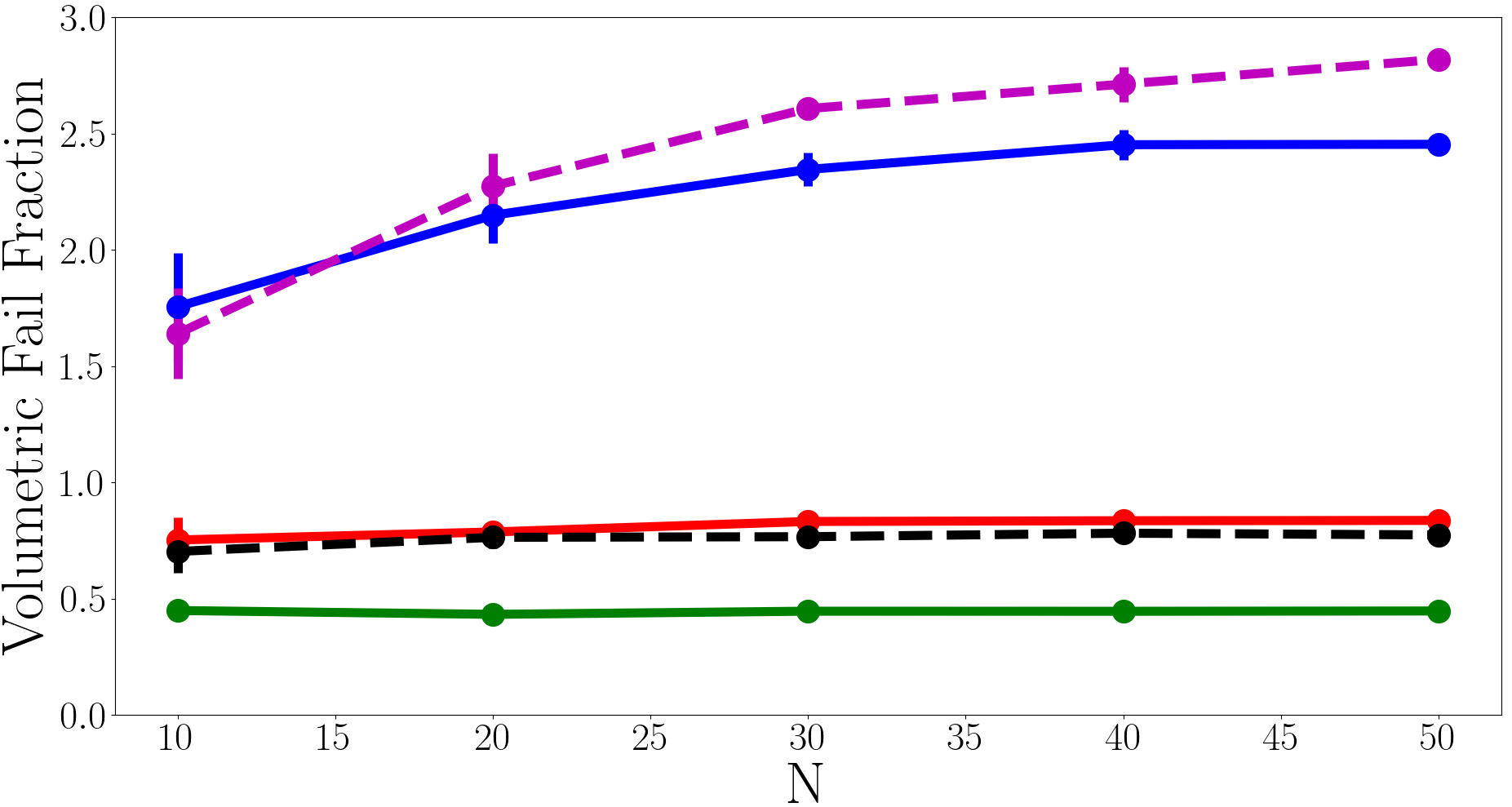

It is important to check whether or not the results of the automaton are convergent or if they are resolution-dependent, i.e. it is important to know how the number of cells () and the size of the frequency decrement () affect the final results.
In Fig. 18 we present the fraction of crust that fails as well as as functions of and . In the first and second panels we see that both quantities converge as a function of . In the third and fourth panels of Fig. 18 we see the fraction of failed crust and also converge with .
We note that the number of events depends quadratically on . The number of cells in the automaton is equal to and as the number of cells increases the size of each individual cell decreases, so a high-strain region of the crust contains more cells, which subsequently fail (meaning more events). However, this does not change the total heat dissipated, nor the amount of crust that fails in practice. Therefore as described in Section 3.1 the cut-offs of the and PDFs depend on and , with higher resolution making smaller events or shorter waiting times possible.
We find that does not significantly affect the behaviour of nor . Both quantities converge to an accuracy of better than 25% per cent for , recall and .
The results presented in the body of this paper are drawn from simulations with and unless otherwise specified.
APPENDIX E: MOMENT OF INERTIA CALCULATION
In this paper the star is made of two components, the solid crust and the fluid core. In addition the crust is broken up into cells as part of the cellular automaton. We calculate the ellipticity and emitted wave strain of the star in Section 4 and so require its moments of inertia. We therefore need the masses and centres of mass of each crustal cell and core segment underneath each cell. Formulas for these quantities are stated for reference in this appendix.
The mass of cell is
| (30) |
and the mass of the fluid segment beneath cell is
| (31) |
The centre of mass is defined as,
| (32) |
where is the total mass of the object, is its volume and is the density. In this case the centre of mass coordinates of cell are given by
| (33) |
Likewise the center-of-mass coordinates of the underlying core segment are given by
| (34) |
Additionally we must consider the edge cases and . When the lower terminal of integration in is and when the upper terminal is for Eqs. (30), (31), (33), and (34). The north and south poles act as the boundaries of the most polar cells. Similarly when considering , the discontinuity in across the positive -axis must be accounted for otherwise we have which is inappropriate; when considering this boundary should be used instead.
Calculating the centres of mass using Eqs. (33) and (34) is computationally expensive. For large the centres of mass are well approximated by
| (35) | ||||
| (36) |
The approximation is used because the computation is approximately three times faster than the exact calculation and the accuracy remains high, viz. a disagreement of for .