Uniform approximation problems of expanding Markov maps

Yubin He Address: Department of Mathematics, South China University of Technology, Guangzhou, Guangdong 510641, P. R. China Email address: yubinhe007@gmail.com and Lingmin Liao Address: School of Mathematics and Statistics, Wuhan University, Wuhan, Hubei 430072, P. R. China Email address: lmliao@whu.edu.cn

Abstract.

Let $T:[0,1]\to[0,1]$ be an expanding Markov map with a finite partition. Let $\mu_{\phi}$ be the invariant Gibbs measure associated with a Hölder continuous potential $\phi$ . In this paper, we investigate the size of the uniform approximation set

\mathcal{U}^{\kappa}(x):=\{y\in[0,1]:\forall N\gg 1,~\exists n\leq N,\text{ such that }|T^{n}x-y|<N^{-\kappa}\},

where $\kappa>0$ and $x\in[0,1]$ . The critical value of $\kappa$ such that $\hdim\mathcal{U}^{\kappa}(x)=1$ for $\mu_{\phi}$ -a.e. $x$ is proven to be $1/\alpha_{\max}$ , where $\alpha_{\max}=-\int\phi\,d\mu_{\max}/\int\log|T^{\prime}|\,d\mu_{\max}$ and $\mu_{\max}$ is the Gibbs measure associated with the potential $-\log|T^{\prime}|$ . Moreover, when $\kappa>1/\alpha_{\max}$ , we show that for $\mu_{\phi}$ -a.e. $x$ , the Hausdorff dimension of $\mathcal{U}^{\kappa}(x)$ agrees with the multifractal spectrum of $\mu_{\phi}$ .

Key words and phrases:

Uniform Diophantine approximation, Markov map, Hausdorff dimension, Gibbs measure, multifractal spectrum

2010 Mathematics Subject Classification

28A80

1. Introduction and motivation

Denote by $\|\cdot\|$ the distance to the nearest integer. The famous Dirichlet Theorem asserts that for any real numbers $x\in[0,1]$ and $N\geq 1$ , there exists a positive integer $n$ such that

(1.1)

\|nx\|<\frac{1}{N}\quad\text{and}\quad n\leq N.

As a corollary, for any $x\in[0,1]$ , there exist infinitely many positive integers $n$ such that

(1.2)

\|nx\|\leq\frac{1}{n}.

Let $(\{nx\})_{n\geq 0}$ be the orbit of $0$ of the irrational rotation by an irrational number $x$ , where $\{nx\}$ is the fractional part of $nx$ . From the dynamical perspective, Dirichlet Theorem and its corollary describe the rate at which $0$ is approximated by the orbit $(\{nx\})_{n\geq 0}$ in a uniform and asymptotic way, respectively.

In general, one can study the Hausdorff dimension of the set of points which are approximated by the orbit $(\{nx\})_{n\geq 0}$ with a faster speed. For the asymptotic approximation, Bugeaud [8] and, independently, Schmeling and Troubetzkoy [27] proved that

\hdim\{y\in[0,1]:\|nx-y\|<n^{-\kappa}\text{ for infinitely many }n\}=\frac{1}{\kappa},

where $\hdim$ stands for the Hausdorff dimension. The corresponding uniform approximation problem was recently studied by Kim and Liao [18] who obtained the Hausdorff dimension of the set

\{y\in[0,1]:\forall N\gg 1,~\exists n\leq N,\text{ such that }\|nx-y\|<N^{-\kappa}\}.

Naturally, one wonders about the analog results when the orbit $(\{nx\})_{n\geq 0}$ is replaced by an orbit $(T^{n}x)_{n\geq 0}$ of a general dynamical system $([0,1],T)$ . For any $\kappa>0$ , Fan, Schmeling and Troubetzkoy [13] considered the set

\mathcal{L}^{\kappa}(x):=\{y\in[0,1]:|T^{n}x-y|<n^{-\kappa}\text{ for infinitely many }n\}

of points that are asymptotically approximated by the orbit $(T^{n}x)_{n\geq 0}$ with a given speed $n^{-\kappa}$ , where $T$ is the doubling map. It seems difficult to investigate the size of $\mathcal{L}^{\kappa}(x)$ when $x$ is not a dyadic rational, as the distribution of $(T^{n}x)_{n\geq 0}$ is not as well-studied as that of $(\{nx\})_{n\geq 0}$ , see for example [1] for more details about the distribution of $(\{nx\})_{n\geq 0}$ . However, from the viewpoint of ergodic theory, Fan, Schmeling and Troubetzkoy [13] obtained the Hausdorff dimension of $\mathcal{L}^{\kappa}(x)$ for $\mu_{\phi}$ -a.e. $x$ , where $\mu_{\phi}$ is the Gibbs measure associated with a Hölder continuous potential $\phi$ . They found that the size of $\mathcal{L}^{\kappa}(x)$ is closely related to the local dimension of $\mu_{\phi}$ and to the first hitting time for shrinking targets.

In their paper [20], Liao and Seuret extended the results of [13] to Markov maps. Later, Persson and Rams [23] considered more general piecewise expanding interval maps, and proved some similar results to those of [13, 20]. These studies are also closed related to the metric theory of random covering set; see [3, 11, 12, 17, 28, 29, 31] and references therein.

As a counterpart of the dynamically defined asymptotic approximation set $\mathcal{L}^{\kappa}(x)$ , we would like to study the corresponding uniform approximation set $\mathcal{U}^{\kappa}(x)$ defined as

\begin{split}\mathcal{U}^{\kappa}(x):&=\{y\in[0,1]:\forall N\gg 1,~\exists n\leq N,\text{ such that }|T^{n}x-y|<N^{-\kappa}\}\\ &=\bigcup_{i=1}^{\infty}\bigcap_{N=i}^{\infty}\bigcup_{n=1}^{N}B(T^{n}x,N^{-\kappa}),\end{split}

where $B(x,r)$ is the open ball of center $x$ and radius $r$ , and $T$ is a Markov map (see Definition 1.1 below).

As the studies on $\mathcal{L}^{\kappa}(x)$ , we are interested in the sizes (Lebesgue measure and Hausdorff dimension) of $\mathcal{U}^{\kappa}(x)$ . By a simple argument, one can check that $\mathcal{U}^{\kappa}(x)\setminus\{T^{n}x\}_{n\geq 0}\subset\mathcal{L}^{\kappa}(x)$ . Thus, trivially one has $\lambda(\mathcal{U}^{\kappa}(x))\leq\lambda(\mathcal{L}^{\kappa}(x))$ and $\hdim\mathcal{U}^{\kappa}(x)\leq\hdim\mathcal{L}^{\kappa}(x)$ . Here, $\lambda$ denotes the Lebesgue measure on $[0,1]$ .

Our first result asserts that for any $\kappa>0$ , the Lebesgue measure and the Hausdorff dimension of $\mathcal{U}^{\kappa}(x)$ are constant almost surely with respect to a $T$ -invariant ergodic measure.

Theorem 1.1.

Let $T$ be a Markov map on $[0,1]$ and $\nu$ be a $T$ -invariant ergodic measure. Then for any $\kappa>0$ , both $\lambda(\mathcal{U}^{\kappa}(x))$ and $\hdim\mathcal{U}^{\kappa}(x)$ are constants almost surely.

To further describe the size of $\mathcal{U}^{\kappa}(x)$ for all most all points, we impose a stronger condition, the same as that of Fan, Schmeling and Troubetzkoy [13] and Liao and Seuret [20], that $\nu$ is a Gibbs measure. Precisely, let $\phi$ be a Hölder continuous potential and $\mu_{\phi}$ be the associated Gibbs meaure. Let $\mathcal{B}^{\kappa}(x):=[0,1]\setminus\mathcal{U}^{\kappa}(x)$ . We remark that the sets $\mathcal{U}^{\kappa}(x)$ are decreasing (the sets $\mathcal{B}^{\kappa}(x)$ are increasing) with respect to $\kappa$ . Then, we want to ask, for $\mu_{\phi}$ almost all points $x$ , how the size of $\mathcal{U}^{\kappa}(x)$ (and $\mathcal{B}^{\kappa}(x)$ ) changes with respect to $\kappa$ . We thus would like to answer the following questions.

(Q1)

When $\mathcal{U}^{\kappa}(x)=[0,1]$ for $\mu_{\phi}$ -a.e. $x$ ? What is the critical value

$\kappa_{\phi}:=\sup\{\kappa\geq 0:\mathcal{U}^{\kappa}(x)=[0,1]\ \text{for $\mu_{\phi}$-a.e.}\,x\}?$
(Q2)

When $\lambda(\mathcal{U}^{\kappa}(x))=1$ for $\mu_{\phi}$ -a.e. $x$ ? What is the critical value

$\kappa_{\phi}^{\lambda}:=\sup\{\kappa\geq 0:\lambda(\mathcal{U}^{\kappa}(x))=1\ \text{for $\mu_{\phi}$-a.e.}\,x\}?$
(Q3)

What are the Hausdorff dimensions of $\mathcal{U}^{\kappa}(x)$ and $\mathcal{B}^{\kappa}(x)$ for $\mu_{\phi}$ -a.e. $x$ ? What are the critical value

$\kappa_{\phi}^{H}:=\sup\{\kappa\geq 0:\hdim(\mathcal{U}^{\kappa}(x))=0\ \text{for $\mu_{\phi}$-a.e.}\,x\}?$

In this paper, we answer these questions when $T$ is an expanding Markov map of the interval $[0,1]$ with a finite partition—a Markov map, for short.

Definition 1.1 (Markov map).

A transformation $T:[0,1]\to[0,1]$ is an expanding Markov map with a finite partition provided that there is a partition of $[0,1]$ into subintervals $I(i)=(a_{i},a_{i+1})$ for $i=0,\dots,Q-1$ with endpoints $0=a_{0}<a_{1}<\cdots<a_{Q}=1$ satisfying the following properties.

(1)

There is an integer $n_{0}$ and a real number $\rho$ such that $|(T^{n_{0}})^{\prime}|\geq\rho>1$ .
(2)

$T$ is strictly monotonic and can be extended to a $C^{2}$ function on each $\overline{I(i)}$ .
(3)

If $I(j)\cap T\big(I(k)\big)\neq\emptyset$ , then $I(j)\subset T\big(I(k)\big)$ .
(4)

There is an integer $R$ such that $I(j)\subset\cup_{n=1}^{R}T^{n}\big(I(k)\big)$ for every $k$ , $j$ .
(5)

For every $k\in\{0,1,\dots,Q-1\}$ , $\sup_{(x,y,z)\in I(k)^{3}}\big(|T^{\prime\prime}(x)|/|T^{\prime}(y)||T^{\prime}(z)|\big)<\infty$ .

For a probability measure $\nu$ on $[0,1]$ and a point $y\in[0,1]$ , we set

\underline{d}_{\nu}(y):=\liminf_{r\to 0}\frac{\log\nu\big(B(y,r)\big)}{\log r}\quad\text{and}\quad\overline{d}_{\nu}(y):=\limsup_{r\to 0}\frac{\log\nu\big(B(y,r)\big)}{\log r},

which are called, respectively, the lower and upper local dimensions of $\nu$ at $y$ . When $\underline{d}_{\nu}(y)=\overline{d}_{\nu}(y)$ , their common value is denoted by $d_{\nu}(y)$ , and is simply called the local dimension of $\nu$ at $y$ . Let $D_{\nu}$ be the multifractal spectrum of $\nu$ defined by

D_{\nu}(s):=\hdim\{y\in[0,1]:d_{\nu}(y)=s\}\quad\forall s\in\mathbb{R}.

Let $T$ be a Markov map as in Definition 1.1 and let $\phi$ be a Hölder continuous potential. Denote by $\mathcal{M}_{\mathrm{inv}}$ the set of $T$ -invariant probability measures on $[0,1]$ and $\mu_{\max}$ the Gibbs measure associated with the potential $-\log|T^{\prime}|$ . Define

(1.3)	$\displaystyle\alpha_{-}:$	$\displaystyle=\min_{\nu\in\mathcal{M}_{\mathrm{inv}}}\frac{-\int\phi\,d\nu}{\int\log\|T^{\prime}\|\,d\nu},$
(1.4)	$\displaystyle\alpha_{\max}:$	$\displaystyle=\frac{-\int\phi\,d\mu_{\max}}{\int\log\|T^{\prime}\|\,d\mu_{\max}},$
(1.5)	$\displaystyle\alpha_{+}:$	$\displaystyle=\max_{\nu\in\mathcal{M}_{\mathrm{inv}}}\frac{-\int\phi\,d\nu}{\int\log\|T^{\prime}\|\,d\nu}.$

By definition, it holds that $\alpha_{-}\leq\alpha_{\max}\leq\alpha_{+}$ . Indeed, the quantities $\alpha_{-}$ , $\alpha_{\max}$ and $\alpha_{+}$ depend on $T$ and $\phi$ . However, for simplicity, we leave out the dependence unless the context requires specification.

The following main theorem tells us that the three critical values demanded in questions (Q1)-(Q3) are $\alpha_{+}$ , $\alpha_{\max}$ and $\alpha_{-}$ , correspondingly.

Theorem 1.2.

Let $T$ be a Markov map. Let $\phi$ be a Hölder continuous potential and $\mu_{\phi}$ be the associated Gibbs measure.

(1)

The critical value $\kappa_{\phi}$ is $\alpha_{+}$ . Namely, for $\mu_{\phi}$ -a.e. $x$ , $\mathcal{U}^{\kappa}(x)=[0,1]$ if $1/\kappa>\alpha_{+}$ , and $\mathcal{U}^{\kappa}(x)\neq[0,1]$ if $1/\kappa<\alpha_{+}$ .

(2)

The critical value $\kappa_{\phi}^{\lambda}$ is $\alpha_{\max}$ . Moreover, for $\mu_{\phi}$ -a.e. $x$ ,

\lambda\big(\mathcal{U}^{\kappa}(x)\big)=1-\lambda\big(\mathcal{B}^{\kappa}(x)\big)=\begin{cases}0\quad&\text{if }1/\kappa\in(0,\alpha_{\max}),\\ 1\quad&\text{if }1/\kappa\in(\alpha_{\max},+\infty).\end{cases}

(3)

The critical value $\kappa_{\phi}^{H}$ is $\alpha_{-}$ . Moreover, for $\mu_{\phi}$ -a.e. $x$ ,

\hdim\mathcal{U}^{\kappa}(x)=\begin{cases}D_{\mu_{\phi}}(1/\kappa)&\text{if }1/\kappa\in(0,\alpha_{\max}]\setminus\{\alpha_{-}\},\\ 1&\text{if }1/\kappa\in(\alpha_{\max},+\infty).\end{cases}

(4)

For $\mu_{\phi}$ -a.e. $x$ ,

\hdim\mathcal{B}^{\kappa}(x)=\begin{cases}1&\text{if }1/\kappa\in(0,\alpha_{\max}),\\ D_{\mu_{\phi}}(1/\kappa)&\text{if }1/\kappa\in[\alpha_{\max},+\infty)\setminus\{\alpha_{+}\}.\end{cases}

Remark 1.

It is worth noting that the multifractal spectrum $D_{\mu_{\phi}}(s)$ vanishes if $s\notin[\alpha_{-},\alpha_{+}]$ . So if $1/\kappa<\alpha_{-}$ , then $\hdim\mathcal{U}^{\kappa}(x)=0$ for $\mu_{\phi}$ -a.e. $x$ .

Remark 2.

The cases $1/\kappa=\alpha_{-}$ and $\alpha_{+}$ are not covered by Theorem 1.2. However, if the multifractal spectrum $D_{\mu_{\phi}}$ is continuous at $\alpha_{-}$ (respectively $\alpha_{+}$ ), we get that $\hdim\mathcal{U}^{\alpha_{-}}(x)=0$ (respectively $\hdim\mathcal{B}^{\alpha_{+}}(x)=0$ ) for $\mu_{\phi}$ -a.e. $x$ . The situation becomes more subtle if $D_{\mu_{\phi}}(\cdot)$ is discontinuous at $\alpha_{-}$ (respectively $\alpha_{+}$ ). Our methods do not work for obtaining the value of $\hdim\mathcal{U}^{\alpha_{-}}(x)$ (respectively $\hdim\mathcal{B}^{\alpha_{+}}(x)$ ) for $\mu_{\phi}$ -a.e. $x$ .

Let $\hdim\nu$ be the dimension of the Borel probability measure $\nu$ defined by

\hdim\nu=\inf\{\hdim E:E\text{ is Borel set of }[0,1]\text{ and }\nu(E)>0\}.

Remark 3.

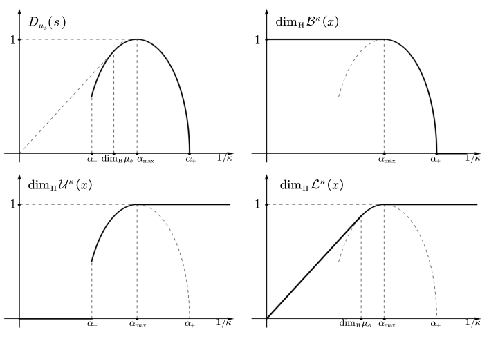
As already discussed above, $\mathcal{U}^{\kappa}(x)\setminus\{T^{n}x\}_{n\geq 0}\subset\mathcal{L}^{\kappa}(x)$ , one may wonder whether the sets $\mathcal{U}^{\kappa}(x)$ and $\mathcal{L}^{\kappa}(x)$ are essentially different. More precisely, is it possible that $\hdim\mathcal{U}^{\kappa}(x)$ is strictly less than $\hdim\mathcal{L}^{\kappa}(x)$ ? Theorem 1.2 affirmatively answers this question. Compared with the asymptotic approximation set $\mathcal{L}^{\kappa}(x)$ , the structure of the uniform approximation set $\mathcal{U}^{\kappa}(x)$ does have a notable feature. When $1/\kappa\in(0,\hdim\mu_{\phi})\setminus\{\alpha_{-}\}$ , the map $1/\kappa\mapsto\hdim\mathcal{U}^{\kappa}(x)$ agrees with the multifractal spectrum $D_{\mu_{\phi}}(1/\kappa)$ , while the map $1/\kappa\mapsto\hdim\mathcal{L}^{\kappa}(x)$ is the linear function $f(1/\kappa)=1/\kappa$ independent of the multifractal spectrum. Therefore, $\hdim\mathcal{U}^{\kappa}(x)<\hdim\mathcal{L}^{\kappa}(x)$ . See Figure 1 for an illustration.

Refer to caption — Figure 1: The multifractal spectrum of $\mu_{\phi}$ and the maps $1/\kappa\mapsto\hdim\mathcal{B}^{\kappa}(x)$ , $1/\kappa\mapsto\hdim\mathcal{U}^{\kappa}(x)$ and $1/\kappa\mapsto\hdim\mathcal{L}^{\kappa}(x)$ .

Remark 4.

For the asymptotic approximation set $\mathcal{L}^{\kappa}(x)$ , the most difficult part lies in establishing the lower bound for $\hdim\mathcal{L}^{\kappa}(x)$ when $1/\kappa<\hdim\mu_{\phi}$ , for which a multifractal mass transference principle for Gibbs measure is applied, see [13, §8], [20, §5.2] and [23, §6]. Specifically, since $\mu_{\phi}(\mathcal{L}^{\delta}(x))=1$ for all $1/\delta>\hdim\mu_{\phi}$ , the multifractal mass transference principle guarantees the lower bound $\hdim\mathcal{L}^{\kappa}(x)\geq(\hdim\mu_{\phi})\delta/\kappa$ for all $1/\kappa<\hdim\mu_{\phi}$ . By letting $1/\delta$ monotonically decrease to $\hdim\mu_{\phi}$ along a sequence $(\delta_{n})$ , we get immediately the expected lower bound $\hdim\mathcal{L}^{\kappa}(x)\geq 1/\kappa$ for all $1/\kappa<\hdim\mu_{\phi}$ . However, recent progresses in uniform approximation [9, 18, 19, 33] indicate that there is no mass transference principle for uniform approximation set. Therefore, we can not expect that $\hdim\mathcal{U}^{\kappa}(x)$ decreases linearly with respect to $1/\kappa$ as $\hdim\mathcal{L}^{\kappa}(x)$ does. The main new ingredient of this paper is the difficult upper bound for $\hdim\mathcal{U}^{\kappa}(x)$ when $1/\kappa<\hdim\mu_{\phi}$ . To overcome the difficulty, we fully develop and combine the methods in [13] and [19].

To illustrate our main theorem, let us give some examples.

Example 1.

Suppose that $T$ is the doubling map and $\mu_{\phi}:=\lambda$ is the Lebesgue measure. Applying Theorem 1.2, we have that for $\lambda$ -a.e. $x$ ,

\hdim\mathcal{U}^{\kappa}(x)=\begin{cases}0&\text{if }1/\kappa\in(0,1),\\ 1&\text{if }1/\kappa\in(1,+\infty).\end{cases}

The Lebesgue measure is monofractal and hence the corresponding multifractal spectrum $D_{\lambda}$ is discontinuous at $1$ . Theorem 1.2 fails to provide any metric statement for the set $\mathcal{U}^{1}(x)$ for $\lambda$ -a.e. $x$ . However, we can conclude that $\mathcal{U}^{1}(x)$ is a Lebesgue null set for $\lambda$ -a.e. $x$ from Fubini Theorem and a zero-one law established in [15, Theorem 2.1]. Further, by Theorem 1.1, $\hdim\mathcal{U}^{1}(x)$ is constant for $\lambda$ -a.e. $x$ .

Some sets similar to $\mathcal{U}^{1}(x)$ in Example 1 have recently been studied by Koivusalo, Liao and Persson [19]. In their paper, instead of the orbit $(T^{n}x)_{n\geq 0}$ , they investigated the sets of points uniformly approximated by an independent and identically distributed sequence $(\omega_{n})_{n\geq 1}$ . Specifically, they showed that with probability one, the lower bound of the Hausdorff dimension of the set

\begin{split}\{y\in[0,1]:\forall N\gg 1,~\exists n\leq N,\text{ such that }|\omega_{n}-y|<1/N\}\end{split}

is larger than $0.2177444298485995$ ([19, Theorem 5]).

Example 2.

Let $p\in(1/2,1)$ . Suppose that $T$ is the doubling map on $[0,1]$ and $\mu_{p}$ is the $(p,1-p)$ Bernoulli measure. It is known that the multifractal spectrum $D_{\mu_{p}}$ is continuous on $(0,+\infty)$ and attains its unique maximal value $1$ at $-\log_{2}\big(p(1-p)\big)/2$ . Theorem 1.2 then gives that for $\mu_{p}$ -a.e. $x$ ,

\hdim\mathcal{U}^{\kappa}(x)=\begin{cases}D_{\mu_{p}}(1/\kappa)&\text{if }1/\kappa\in\bigg(0,\frac{-\log_{2}\big(p(1-p)\big)}{2}\bigg),\\ 1&\text{if }1/\kappa\in\bigg[\frac{-\log_{2}\big(p(1-p)\big)}{2},+\infty\bigg).\end{cases}

Our paper is organized as follows. We start in Section 2 with some preparations on Markov map, and then apply ergodic theory to give a proof of Theorem 1.1. Section 3 contains some recalls on multifractal analysis and a variational principle which are essential in the proof of Theorem 1.2. Section 4 describes some relations among hitting time, approximating rate and local dimension of $\mu_{\phi}$ . From these relations we then derive items (1), (2) and (4) of Theorem 1.2 in Section 5.1, as well as the lower bound of $\hdim\mathcal{U}^{\kappa}(x)$ in Section 5.2. In the same Section 5.2, we establish the upper bound of $\hdim\mathcal{U}^{\kappa}(x)$ , which is arguably the most substantial part.

2. Basic definitions and the proof of Theorem 1.1

2.1. Covering of $[0,1]$ by basic intervals

Let $T$ be a Markov map as defined in Definition 1.1. For each $(i_{1}i_{2}\cdots i_{n})\in\{0,1,\dots,Q-1\}^{n}$ , we call

I(i_{1}i_{2}\cdots i_{n}):=I(i_{1})\cap T^{-1}\big(I(i_{2})\big)\cap\dots\cap T^{-n+1}\big(I(i_{n})\big)

a basic interval of generation $n$ . It is possible that $I(i_{1}i_{2}\cdots i_{n})$ is empty for some $(i_{1}i_{2}\cdots i_{n})\in\{0,1,\dots,Q-1\}^{n}$ . The collection of non-empty basic intervals of a given generation $n$ will be denoted by $\Sigma_{n}$ . For any $x\in[0,1]$ , we denote $I_{n}(x)$ the unique basic interval $I\in\Sigma_{n}$ containing $x$ .

By the definition of Markov map, we obtain the following bounded distortion property on basic intervals: there is a constant $L>1$ such that for any $x\in[0,1]$ ,

(2.1)

\text{for any }n\geq 1,\quad L^{-1}|(T^{n})^{\prime}(x)|^{-1}\leq|I_{n}(x)|\leq L|(T^{n})^{\prime}(x)|^{-1},

where $|I|$ is the length of the interval $I$ . Consequently, we can find two constants $1<L_{1}<L_{2}$ such that

(2.2)

\text{for every }I\in\Sigma_{n},\quad L_{2}^{-n}\leq|I|\leq L_{1}^{-n}.

2.2. Proof of Theorem 1.1

Let us start with a simple but crucial observation.

Lemma 2.1.

Let $T$ be a Markov map. For any $\kappa>0$ , we have $\mathcal{U}^{\kappa}(x)\setminus\{Tx\}\subset\mathcal{U}^{\kappa}(Tx)$ .

Proof.

Let $y\in\mathcal{U}^{\kappa}(x)\setminus\{Tx\}$ and let $i$ be the smallest integer satisfying $y\notin B(Tx,2^{-i\kappa})$ . By the definition of $\mathcal{U}^{\kappa}(x)$ , for any integer $N>2^{i}$ large enough, there exists $1\leq n\leq N$ such that $y\in B(T^{n}x,N^{-\kappa})$ . Moreover, the condition $N>2^{i}$ implies that $n\neq 1$ , hence $y\in B\big(T^{n-1}(Tx),N^{-\kappa}\big)$ . This gives that $y\in\mathcal{U}^{\kappa}(Tx)$ . Therefore, $\mathcal{U}^{\kappa}(x)\setminus\{Tx\}\subset\mathcal{U}^{\kappa}(Tx)$ . ∎

Recall that a $T$ -invariant measure $\nu$ is ergodic if and only if any $T$ -invariant function is constant almost surely. The proof of Theorem 1.1 falls naturally into two parts. We first deal with the Lebesgue measure part.

Proof of Theorem 1.1: Lebesgue measure part.

For any $\kappa>0$ , define the function $g_{\kappa}:x\mapsto\lambda(\mathcal{U}^{\kappa}(x))$ . We claim that $g_{\kappa}$ is measurable. In fact, it suffices to observe that

g_{\kappa}(x)=\lim_{i\to\infty}\lim_{m\to\infty}\lambda\bigg(\bigcap_{N=i}^{m}\bigcup_{n=1}^{N}B(T^{n}x,N^{-\kappa})\bigg)

and that, by the piecewise continuity of $T^{n}$ ( $n\geq 1$ ), the set

\bigg\{x\in[0,1]:\lambda\bigg(\bigcap_{N=i}^{m}\bigcup_{n=1}^{N}B(T^{n}x,N^{-\kappa})\bigg)>t\bigg\}

is measurable for any $t\in\mathbb{R}$ .

By Lemma 2.1, we see that $\lambda(\mathcal{U}^{\kappa}(Tx))\geq\lambda(\mathcal{U}^{\kappa}(x))$ , or equivalently, $g_{\kappa}(Tx)\geq g_{\kappa}(x)$ . Since $g_{\kappa}$ is measurable, by the fact $0\leq g_{\kappa}\leq 1$ and the invariance of $\nu$ , we have that $g_{\kappa}$ is invariant with repect to $\nu$ , that is, $g_{\kappa}(Tx)=g_{\kappa}(x)$ for $\nu$ -a.e. $x$ . In the presence of ergodicity of $\nu$ , $g_{\kappa}$ is constant almost surely. ∎

Proof of Theorem 1.1: Hausdorff dimension part.

Fix $\kappa>0$ , define the function $f_{\kappa}:x\mapsto\hdim\mathcal{U}^{\kappa}(x)$ . Again by Lemma 2.1, we see that $f_{\kappa}(Tx)\geq f_{\kappa}(x)$ . Proceed in the same way as in the Lebesgue measure part yields that $f_{\kappa}$ is constant almost surely provided that $f_{\kappa}$ is measurable.

To show that $f_{\kappa}$ is measurable, it suffices to prove that for any $t>0$ , the set

\begin{split}A(t):=\{x\in[0,1]:f_{\kappa}(x)<t\}=\bigg\{x\in[0,1]:\hdim\bigg(\bigcup_{i=1}^{\infty}\bigcap_{N=i}^{\infty}\bigcup_{n=1}^{N}B(T^{n}x,N^{-\kappa})\bigg)<t\bigg\}\end{split}

is measurable. Through out the proof of this part, we will assume that the ball $B(T^{n}x,N^{-\kappa})$ is closed. This makes the proof achievable, and it does not change the Hausdorff dimension of $\mathcal{U}^{\kappa}(x)$ .

By the definition of Hausdorff dimension, a point $x\in A(t)$ if and only if there exists $h\in\mathbb{N}$ such that

\mathcal{H}^{t-\frac{1}{h}}\bigg(\bigcup_{i=1}^{\infty}\bigcap_{N=i}^{\infty}\bigcup_{n=1}^{N}B(T^{n}x,N^{-\kappa})\bigg)=0,

or equivalently for all $i\geq 1$ ,

(2.3)

\mathcal{H}^{t-\frac{1}{h}}\bigg(\bigcap_{N=i}^{\infty}\bigcup_{n=1}^{N}B(T^{n}x,N^{-\kappa})\bigg)=0.

By the definition of Hausdorff measure, (2.3) holds if and only if for any $j,k\in\mathbb{N}$ ,

\mathcal{H}_{\frac{1}{j}}^{t-\frac{1}{h}}\bigg(\bigcap_{N=i}^{\infty}\bigcup_{n=1}^{N}B(T^{n}x,N^{-\kappa})\bigg)<\frac{1}{k}.

Hence, we see that

\begin{split}A(t)=\bigcup_{h=1}^{\infty}\bigcap_{i=1}^{\infty}\bigcap_{j=1}^{\infty}\bigcap_{k=1}^{\infty}\bigg\{x\in[0,1]:\mathcal{H}_{\frac{1}{j}}^{t-\frac{1}{h}}\bigg(\bigcap_{N=i}^{\infty}\bigcup_{n=1}^{N}B(T^{n}x,N^{-\kappa})\bigg)<\frac{1}{k}\bigg\}=:\bigcup_{h=1}^{\infty}\bigcap_{i=1}^{\infty}\bigcap_{j=1}^{\infty}\bigcap_{k=1}^{\infty}B_{h,i,j,k}.\end{split}

If $x\in B_{h,i,j,k}$ , then there is a countable open cover $\{U_{p}\}_{p\geq 1}$ with $0<|U_{p}|<1/j$ satisfying

(2.4)

\bigcap_{N=i}^{\infty}\bigcup_{n=1}^{N}B(T^{n}x,N^{-\kappa})\subset\bigcup_{p=1}^{\infty}U_{p}\quad\text{and}\quad\sum_{p=1}^{\infty}|U_{p}|^{t-\frac{1}{h}}<\frac{1}{k}.

The set $\bigcap_{N=i}^{\infty}\bigcup_{n=1}^{N}B(T^{n}x,N^{-\kappa})$ can be viewed as the intersection of a family of decreasing compact sets $\big\{\bigcap_{N=i}^{l}\bigcup_{n=1}^{N}B(T^{n}x,N^{-\kappa})\big\}_{l\geq i}$ . Hence there exists $l_{0}\geq i$ satisfying

\bigcap_{N=i}^{l_{0}}\bigcup_{n=1}^{N}B(T^{n}x,N^{-\kappa})\subset\bigcup_{p=1}^{\infty}U_{p},

which implies

\mathcal{H}_{\frac{1}{j}}^{t-\frac{1}{h}}\bigg(\bigcap_{N=i}^{l_{0}}\bigcup_{n=1}^{N}B(T^{n}x,N^{-\kappa})\bigg)<\frac{1}{k}.

We then deduce that

(2.5)

B_{h,i,j,k}\subset\bigcup_{l=i}^{\infty}\bigg\{x\in[0,1]:\mathcal{H}_{\frac{1}{j}}^{t-\frac{1}{h}}\bigg(\bigcap_{N=i}^{l}\bigcup_{n=1}^{N}B(T^{n}x,N^{-\kappa})\bigg)<\frac{1}{k}\bigg\}=:\bigcup_{l=i}^{\infty}C_{h,i,j,k,l}.

If $x\in C_{h,i,j,k,l}$ for some $l\geq 1$ , then

\mathcal{H}_{\frac{1}{j}}^{t-\frac{1}{h}}\bigg(\bigcap_{N=i}^{\infty}\bigcup_{n=1}^{N}B(T^{n}x,N^{-\kappa})\bigg)\leq\mathcal{H}_{\frac{1}{j}}^{t-\frac{1}{h}}\bigg(\bigcap_{N=i}^{l}\bigcup_{n=1}^{N}B(T^{n}x,N^{-\kappa})\bigg)<\frac{1}{k}.

Hence $x\in B_{i,j,k,l}$ and the reverse inclusion of (2.5) is proved.

Notice that $T,T^{2},\dots,T^{l}$ are continuous on every basic interval of generation greater than $l$ . For any $x\in C_{h,i,j,k,l}$ , denote

\mathcal{S}(x):=\bigcap_{N=i}^{l}\bigcup_{n=1}^{N}B(T^{n}x,N^{-\kappa}).

There is an open cover $(V_{p})_{p\geq 1}$ of $\mathcal{S}(x)$ with $0<|V_{p}|<1/j$ and $\sum_{p}|V_{p}|^{t-1/h}<1/k$ . Since $\mathcal{S}(x)$ is compact, we see that the distance $\delta$ between $\mathcal{S}(x)$ and the complement of $\bigcup_{p\geq 1}V_{p}$ is positive. By the continuities of $T,T^{2},\dots,T^{l}$ , there is some $l_{1}:=l_{1}(\delta)>l$ , for which if $y\in I_{l_{1}}(x)$ , then $\mathcal{S}(y)$ is contained in a $\delta/2$ -neighborhood of $\mathcal{S}(x)$ . Thus $\mathcal{S}(y)$ can also be covered by $\bigcup_{p\geq 1}V_{p}$ , and $I_{l_{1}}(x)\subset C_{h,i,j,k,l}$ . Finally, $C_{h,i,j,k,l}$ is a union of some basic intervals, which is measurable.

Now combining the equalities obtained above, we have

A(t)=\bigcup_{h=1}^{\infty}\bigcap_{i=1}^{\infty}\bigcap_{j=1}^{\infty}\bigcap_{k=1}^{\infty}\bigcup_{l=i}^{\infty}C_{h,i,j,k,l},

which is a Borel measurable set. ∎

3. Multifractal properties of Gibbs measures

In this section, we review some standard facts on multifractal properties of Gibbs measures.

Definition 3.1.

A Gibbs measure $\mu_{\phi}$ associated with a potential $\phi$ is a probability measure satisfying the following: there exists a constant $\gamma>0$ such that

\text{for any basic interval }I\in\Sigma_{n},\quad\gamma^{-1}\leq\frac{\mu_{\phi}(I)}{e^{S_{n}\phi(x)-nP(\phi)}}\leq\gamma,\quad\text{for every }x\in I,

where $S_{n}\phi(x)=\phi(x)+\cdots+\phi(T^{n-1}x)$ is the $n$ th Birkhoff sum of $\phi$ at $x$ , and $P(\phi)$ is the topological pressure of $\phi$ defined by

P(\phi)=\lim_{n\to\infty}\frac{1}{n}\log\sum_{I\in\Sigma_{n}}\sup_{x\in I}e^{S_{n}\phi(x)}.

The following theorem ensures the existence and uniqueness of invariant Gibbs measure.

Theorem 3.1 ([2, 32]).

Let $T:[0,1]\to[0,1]$ be a Markov map. Then for any Hölder continuous function $\phi$ , there exists a unique $T$ -invariant Gibbs measure $\mu_{\phi}$ associated with $\phi$ . Further, $\mu_{\phi}$ is ergodic.

The Gibbs measure $\mu_{\phi}$ also satisfies the quasi-Bernoulli property (see [20, Lemma 4.1]), i.e. for any $n>k\geq 1$ , for any basic interval $I(i_{1}\cdots i_{n})\in\Sigma_{n}$ , the following holds

(3.1)

\gamma^{-3}\mu_{\phi}(I^{\prime})\mu_{\phi}(I^{\prime\prime})\leq\mu_{\phi}(I)=\mu_{\phi}(I^{\prime}\cap T^{-k}I^{\prime\prime})\leq\gamma^{3}\mu_{\phi}(I^{\prime})\mu_{\phi}(I^{\prime\prime}),

where $I^{\prime}=I(i_{1}\cdots i_{k})\in\Sigma_{k}$ and $I^{\prime\prime}=I(i_{k+1}\cdots i_{n})\in\Sigma_{n-k}$ . It follows immediately that

(3.2)

\text{for any }m\geq k,\quad\mu_{\phi}(I^{\prime}\cap T^{-m}U)\leq\gamma^{3}\mu_{\phi}(I^{\prime})\mu_{\phi}(U),

where $U$ is an open set in $[0,1]$ .

We adopt the convention that $\phi$ is normalized, i.e. $P(\phi)=0$ . If it is not the case, we can replace $\phi$ by $\phi-P(\phi)$ .

Now, let us recall some standard facts on multifractal analysis which aims at studying the multifractal spectrum $D_{\mu_{\phi}}$ . Some multifractal analysis results were summarised in [20] and we present them as follows. The proofs can also be found in the references [4, 7, 10, 24, 25, 30].

Theorem 3.2 ([20, Theorem 2.5]).

Let $T$ be a Markov map. Let $\phi$ be a Hölder continuous potential and $\mu_{\phi}$ be the associated Gibbs measure. Then, the following hold.

(1)

The function $D_{\mu_{\phi}}$ of $\mu_{\phi}$ is a concave real-analytic map on the interval $(\alpha_{-},\alpha_{+})$ , where $\alpha_{-}$ and $\alpha_{+}$ are defined in (1.3) and (1.5), respectively.
(2)

The spectrum $D_{\mu_{\phi}}$ reaches its maximum value $1$ at $\alpha_{\max}$ defined in (1.4).
(3)

The graph of $D_{\mu_{\phi}}$ and the first bisector intersect at a unique point which is $(\hdim\mu_{\phi},\hdim\mu_{\phi})$ . Moreover, $\hdim\mu_{\phi}$ satisfies

$\hdim\mu_{\phi}=\frac{-\int\phi\,d\mu_{\phi}}{\int\log|T^{\prime}|\,d\mu_{\phi}}.$

Proposition 3.3 ([20, §2.3]).

For every $q\in\mathbb{R}$ , there is a unique real number $\eta_{\phi}(q)$ such that the topological pressure $P\big(-\eta_{\phi}(q)\log|T^{\prime}|+q\phi\big)$ equals to $0$ . Further, $\eta_{\phi}(q)$ is real-analytic and concave.

Remark 5.

For simplicity, we denote by $\mu_{q}$ the $T$ -invariant Gibbs measure associated with the potential $-\eta_{\phi}(q)\log|T^{\prime}|+q\phi$ . Certainly, $\eta_{\phi}(0)=1$ and the corresponding measure $\mu_{0}$ is associated with the potential $-\log|T^{\prime}|$ . By the bounded distortion property (2.1), the Gibbs measure $\mu_{0}$ , coinciding with $\mu_{\max}$ , is strongly equivalent to the Lebesgue measure $\lambda$ .

For every $q\in\mathbb{R}$ , we introduce the exponent

(3.3)

\alpha(q)=\frac{-\int\phi\,d\mu_{q}}{\int\log|T^{\prime}|\,d\mu_{q}}.

Proposition 3.4 ([20, §2.3]).

Let $\mu_{q}$ and $\alpha(q)$ be as above. The following statements hold.

(1)

The Gibbs measure $\mu_{q}$ is supported by the level set $\{y:d_{\mu_{\phi}}(y)=\alpha(q)\}$ and $D_{\mu_{\phi}}\big(\alpha(q)\big)=\hdim\mu_{q}=\eta_{\phi}(q)+q\alpha(q)$ .

(2)

The map $\alpha(q)$ is decreasing, and

	$\displaystyle\lim_{q\to+\infty}\alpha(q)=\alpha_{-},$	$\displaystyle\quad\lim_{q\to-\infty}\alpha(q)=\alpha_{+},$
	$\displaystyle\alpha(1)=\hdim\mu_{\phi},$	$\displaystyle\ \ \quad\alpha(0)=\alpha_{\max}.$

(3)

The inverse of $\alpha(q)$ exists, and is denoted by $q(\alpha)$ . Moreover, $q(\alpha)<0$ if $\alpha\in(\alpha_{\max},\alpha_{+})$ , and $q(\alpha)\geq 0$ if $\alpha\in(\alpha_{-},\alpha_{\max}]$ .

For a probability measure $\nu$ on $[0,1]$ and a point $y\in[0,1]$ , define the lower and upper Markov pointwise dimensions respectively by

\underline{M}_{\nu}(y):=\liminf_{n\to\infty}\frac{\log\nu\big(I_{n}(y)\big)}{\log|I_{n}(y)|},\quad\overline{M}_{\nu}(y):=\limsup_{n\to\infty}\frac{\log\nu\big(I_{n}(y)\big)}{\log|I_{n}(y)|}.

When $\underline{M}_{\nu}(y)=\overline{M}_{\nu}(y)$ , their common value is denoted by $M_{\nu}(y)$ . By (2.1) and (2.2), we have

\overline{d}_{\nu}(y)\leq\overline{M}_{\nu}(y),

which implies the inclusions

(3.4)

\{y:d_{\nu}(y)=s\}\subset\{y:\underline{d}_{\nu}(y)\geq s\}\subset\{y:\overline{d}_{\nu}(y)\geq s\}\subset\{y:\overline{M}_{\nu}(y)\geq s\}.

By the Gibbs property of $\mu_{\phi}$ and the bounded distortion property on basic intervals (2.1), the definitions of Markov pointwise dimensions can be reformulated as

(3.5)

\overline{M}_{\mu_{\phi}}(y)=\limsup_{n\to\infty}\frac{S_{n}\phi(y)}{S_{n}(-\log T^{\prime})(y)}\quad\text{and}\quad M_{\mu_{\phi}}(y)=\lim_{n\to\infty}\frac{S_{n}\phi(y)}{S_{n}(-\log T^{\prime})(y)}.

This allows us to derive the following lemma, which is an alternative version of a proposition due to Jenkinson [16, Proposition 2.1]. We omit its proof since the argument is similar.

Lemma 3.5.

Let $T$ be a Markov map. Let $\phi$ be a Hölder continuous potential and let $\mu_{\phi}$ be the corresponding Gibbs measure. Then,

\sup_{y\in[0,1]}\overline{M}_{\mu_{\phi}}(y)=\sup_{y\colon M_{\mu_{\phi}}(y)\text{ exists}}M_{\mu_{\phi}}(y)=\max_{\nu\in\mathcal{M}_{\mathrm{inv}}}\frac{-\int\phi\,d\nu}{\int\log|T^{\prime}|\,d\nu}=\alpha_{+}.

In particular, for any $s>\alpha_{+}$ ,

\{y:d_{\mu_{\phi}}(y)=s\}=\{y:\overline{d}_{\mu_{\phi}}(y)\geq s\}=\emptyset.

We finish the section with a variational principle.

Lemma 3.6.

Let $T$ be a Markov map. Let $\phi$ be a Hölder continuous potential and $\mu_{\phi}$ be the associated Gibbs measure.

(1)

For every $s<\alpha_{\max}$ ,

$\hdim\{y:\underline{d}_{\mu_{\phi}}(y)\leq s\}=\hdim\{y:\overline{d}_{\mu_{\phi}}(y)\leq s\}=D_{\mu_{\phi}}(s).$
(2)

For every $s\in(\alpha_{\max},+\infty)\setminus\alpha_{+}$ ,

$\hdim\{y:\underline{d}_{\mu_{\phi}}(y)\geq s\}=\hdim\{y:\overline{d}_{\mu_{\phi}}(y)\geq s\}=D_{\mu_{\phi}}(s).$

Proof.

(1) We point out that the following inclusions hold

\{y:d_{\mu_{\phi}}(y)=s\}\subset\{y:\overline{d}_{\mu_{\phi}}(y)\leq s\}\subset\{y:\underline{d}_{\mu_{\phi}}(y)\leq s\}.

In [20, proposition 2.8], the leftmost set and the rightmost set were shown to have the same Hausdorff dimension. This together with the above inclusions completes the proof of the first point of the lemma.

(2) When $T$ is the doubling map, the statement was formulated by Fan, Schmeling and Trobetzkoy [13, Theorem 3.3]. Our proof follows their idea closely, we include it for completeness.

By Lemma 3.5, we can assume without loss of generality that $s<\alpha_{+}$ . The inclusions in (3.4) imply the following inequalities:

\hdim\{y:d_{\mu_{\phi}}(y)=s\}\leq\hdim\{y:\overline{d}_{\mu_{\phi}}(y)\geq s\}\leq\hdim\{y:\overline{M}_{\mu_{\phi}}(y)\geq s\}.

We turn to prove the reverse inequalites. By Proposition 3.4 and the condition $s>\alpha_{\max}$ , there exists a real number $q_{s}:=q(s)<0$ such that

s=\frac{-\int\phi\,d\mu_{q_{s}}}{\int\log|T^{\prime}|\,d\mu_{q_{s}}}\quad\text{ and }\quad D_{\mu_{\phi}}(s)=\hdim\mu_{q_{s}}=\eta_{\phi}(q_{s})+q_{s}s,

where $\mu_{q_{s}}$ is the Gibbs measure associated with the potential $-\eta_{\phi}(q_{s})\log|T^{\prime}|+q_{s}\phi$ . Now let $y$ be any point such that $\overline{M}_{\mu_{\phi}}(y)\geq s$ . By Proposition 3.3, the topological pressure $P(-\eta_{\phi}(q_{s})\log|T^{\prime}|+q_{s}\phi)$ is $0$ . Then we can apply the Gibbs property of $\mu_{q_{s}}$ and (2.1) to yield

\begin{split}\underline{M}_{\mu_{q_{s}}}(y)&=\liminf_{n\to\infty}\frac{\log e^{S_{n}(-\eta_{\phi}(q_{s})\log|T^{\prime}|+q_{s}\phi)(y)}}{\log|I_{n}(y)|}\\ &=\liminf_{n\to\infty}\bigg(\frac{-\eta_{\phi}(q_{s})\log|(T^{n})^{\prime}(y)|}{\log|I_{n}(y)|}+q_{s}\cdot\frac{\log e^{S_{n}\phi(y)}}{\log|I_{n}(y)|}\bigg)\\ &=\eta_{\phi}(q_{s})+q_{s}\cdot\limsup_{n\to\infty}\frac{\log\mu_{\phi}\big(I_{n}(y)\big)}{\log|I_{n}(y)|}\\ &=\eta_{\phi}(q_{s})+q_{s}\overline{M}_{\mu_{\phi}}(y)\\ &\leq\eta_{\phi}(q_{s})+q_{s}s=D_{\mu_{\phi}}(s),\end{split}

where the inequality holds because $q_{s}<0$ .

Finally, Billingsley’s Lemma [5, Lemma 1.4.1] gives

\hdim\{y:\overline{M}_{\mu_{\phi}}(y)\geq s\}\leq\hdim\{y:\underline{M}_{\mu_{q_{s}}}(y)\leq D_{\mu_{\phi}}(s)\}\leq D_{\mu_{\phi}}(s)=\hdim\{y:d_{\mu_{\phi}}(y)=s\}.\qed

4. Covering questions related to hitting time and local dimension

In Section 4.1 below, we reformulate the uniform approximation set $\mathcal{U}^{\kappa}(x)$ in terms of hitting time. Thereafter, we relate the first hitting time for shrinking balls to the local dimensions in Section 4.2.

4.1. Covering questions and hitting time

Denote $\mathcal{O}^{+}(x):=\{T^{n}x:n\geq 1\}$ .

Definition 4.1.

For every $x,y\in[0,1]$ and $r>0$ , we define the first hitting time of the orbit of $x$ into the ball $B(y,r)$ by

\tau_{r}(x,y):=\inf\{n\geq 1:T^{n}x\in B(y,r)\}.

Set

\underline{R}(x,y):=\liminf_{r\to 0}\frac{\log\tau_{r}(x,y)}{-\log r}\quad\text{and}\quad\overline{R}(x,y):=\limsup_{r\to 0}\frac{\log\tau_{r}(x,y)}{-\log r}.

For convenience, when $\mathcal{O}^{+}(x)\cap B(y,r)=\emptyset$ , we set $\tau_{r}(x,y)=\infty$ and $\underline{R}(x,y)=\overline{R}(x,y)=\infty$ . If $\underline{R}(x,y)=\overline{R}(x,y)$ , we denote the common value by $R(x,y)$ .

For any ball $B\subset[0,1]$ , we define the first hitting time $\tau(x,B)$ by

\tau(x,B):=\inf\{n\geq 1:T^{n}x\in B\}.

Similarly, we set $\tau(x,B)=\infty$ when $\mathcal{O}^{+}(x)\cap B=\emptyset$ .

The following lemma exhibits a relation between $\mathcal{U}^{\kappa}(x)$ and hitting time.

Lemma 4.1.

For any $\kappa>0$ , we have

	$\displaystyle\bigg\{y\in[0,1]:\overline{R}(x,y)>\frac{1}{\kappa}\bigg\}$	$\displaystyle\subset\mathcal{B}^{\kappa}(x)\subset\bigg\{y\in[0,1]:\overline{R}(x,y)\geq\frac{1}{\kappa}\bigg\},$
	$\displaystyle\bigg\{y\in[0,1]:\overline{R}(x,y)<\frac{1}{\kappa}\bigg\}$	$\displaystyle\subset\mathcal{U}^{\kappa}(x)\subset\bigg\{y\in[0,1]:\overline{R}(x,y)\leq\frac{1}{\kappa}\bigg\}.$

Proof.

The top left and bottom right inclusions imply one another. Let us prove the bottom right inclusion. Suppose that $y\in\mathcal{U}^{\kappa}(x)$ . Then for all large enough $N$ there is an $n\leq N$ such that $T^{n}x\in B(y,N^{-\kappa})$ . Thus $\tau_{N^{-\kappa}}(x,y)\leq N$ for all $N$ large enough, which implies $\overline{R}(x,y)\leq 1/\kappa$ .

The top right and bottom left inclusions imply one another. So, it remains to prove the bottom left inclusion. Consider $y$ such that $\overline{R}(x,y)<1/\kappa$ . If $y\in\mathcal{O}^{+}(x)$ with $y=T^{n_{0}}x$ for some $n_{0}\geq 1$ , then the system

|T^{n}x-y|=|T^{n}x-T^{n_{0}}x|<N^{{}_{\kappa}}\quad\text{and}\quad 1\leq n\leq N

always has a trivial solution $n=n_{0}$ for all $N\geq n_{0}$ . Therefore $y\in\mathcal{U}^{\kappa}(x)$ . Now assume that $y\notin\mathcal{O}^{+}(x)$ . By the definition of $\overline{R}(x,y)$ , there is a positive real number $r_{0}<1$ such that

\tau_{r}(x,y)<r^{-1/\kappa},\quad\text{for all }0<r<r_{0}.

Denote $n_{r}:=\tau_{r}(x,y)$ , for all $0<r<r_{0}$ . Since $y\notin\mathcal{O}^{+}(x)$ , the family of positive integers $\{n_{r}:0<r<r_{0}\}$ is unbounded. For each $N>r_{0}^{-1/\kappa}$ , denote $t:=N^{-\kappa}$ . The definition of $n_{t}$ implies that

T^{n_{t}}x\in B(y,t)=B(y,N^{-\kappa}).

We conclude $y\in\mathcal{U}^{\kappa}(x)$ by noting that $n_{t}<t^{-1/\kappa}=N$ . ∎

4.2. Relation between hitting time and local dimension

As Lemma 4.1 shows, we need to study the hitting time $\overline{R}(x,y)$ of the Gibbs measure $\mu_{\phi}$ . We will prove that the hitting time is related to local dimension when the measure is exponential mixing.

Definition 4.2.

A $T$ -invariant measure $\nu$ is exponential mixing if there exist two constants $C>0$ and $0<\beta<1$ such that for any ball $A$ and any Borel measurable set $B$ ,

(4.1)

|\nu(A\cap T^{-n}B)-\nu(A)\nu(B)|\leq C\beta^{n}\nu(B).

Theorem 4.2 ([2, 21, 22, 26]).

The $T$ -invariant Gibbs measure $\mu_{\phi}$ associated with a Hölder continuous potential $\phi$ of a Markov map $T$ is exponential mixing.

The exponential mixing property allows us to apply the following theorem which decribes a relation between hitting time and local dimension of invariant measure.

Theorem 4.3 ([14]).

Let $(X,T,\nu)$ be a measure-theoretic dynamical system. If $\nu$ is superpolynomial mixing and if $d_{\nu}(y)$ exists, then for $\nu$ -a.e. $x$ , we have

R(x,y)=d_{\nu}(y).

It should be noticed that superpolynomial mixing property is much weaker than exponential mixing property.

Now, we turn to the study of the Markov map $T$ on the interval $[0,1]$ . An application of Fubini’s theorem yields the following corollary.

Corollary 4.4 ([20, Corollary 3.8]).

Let $T$ be a Markov map. Let $\mu_{\phi}$ and $\mu_{\psi}$ be two $T$ -invariant Gibbs probability measures on $[0,1]$ associated with Hölder potentials $\phi$ and $\psi$ , respectively. Then,

\text{for }\mu_{\phi}\times\mu_{\psi}\text{-a.e.\,}(x,y),\quad R(x,y)=d_{\mu_{\phi}}(y)=\frac{-\int\phi\,d\mu_{\psi}}{\int\log|T^{\prime}|\,d\mu_{\psi}}.

5. Studies of $\mathcal{B}^{\kappa}(x)$ and $\mathcal{U}^{\kappa}(x)$

5.1. The study of $\mathcal{B}^{\kappa}(x)$

In this subsection, we are going to prove Theorem 1.2 except the item (3). Let us start with the lower bound for $\hdim\mathcal{B}^{\kappa}(x)$ .

Lemma 5.1.

Let $T$ be a Markov map. Let $\phi$ be a Hölder continuous potential and let $\mu_{\phi}$ be the corresponding Gibbs measure. For any $\kappa>0$ , the following hold.

(a)

If $1/\kappa\in(0,\alpha_{\max})$ , then $\lambda\big(\mathcal{B}^{\kappa}(x)\big)=1$ for $\mu_{\phi}$ -a.e. $x$ .
(b)

If $1/\kappa\in[\alpha_{\max},+\infty)\setminus\{\alpha_{+}\}$ , then $\hdim\mathcal{B}^{\kappa}(x)\geq D_{\mu_{\phi}}(1/\kappa)$ for $\mu_{\phi}$ -a.e. $x$ .

Proof.

(a) Let $1/\kappa\in(0,\alpha_{\max})$ . As already observed in Section 3, the Gibbs measure $\mu_{0}$ associated with $\log|T^{\prime}|$ is strongly equivalent to the Lebesgue measure $\lambda$ . Thus, a set $F$ has full $\mu_{0}$ -measure if and only if $F$ has full $\lambda$ -measure. Corollary 4.4 implies that

\text{for }\mu_{\phi}\times\mu_{0}\text{-}a.e.\,(x,y),\quad R(x,y)=d_{\mu_{\phi}}(y)=\frac{-\int\phi\,d\mu_{0}}{\int\log|T^{\prime}|\,d\mu_{0}}=\alpha_{\max}.

By Fubini’s theorem, for $\mu_{\phi}$ -a.e. $x$ , the set $\{y:R(x,y)=d_{\mu_{\phi}}(y)=\alpha_{\max}\}$ has full $\mu_{0}$ -measure. Then for $\mu_{\phi}$ -a.e. $x$ , we have

\mu_{0}\big(\{y:\overline{R}(x,y)>1/\kappa\}\big)\geq\mu_{0}\big(\{y:R(x,y)=d_{\mu_{\phi}}(y)=\alpha_{\max}\}\big)=1.

By Lemma 4.1, we arrive at the conclusion.

(b) By Lemma 3.5, the level set $\{y:d_{\mu_{\phi}}(y)=1/\kappa\}$ is empty if $1/\kappa>\alpha_{+}$ . Thus $D_{\mu_{\phi}}(1/\kappa)=0$ , and therefore $\hdim\mathcal{B}^{\kappa}(x)\geq 0=D_{\mu_{\phi}}(1/\kappa)$ trivially holds for all $1/\kappa>\alpha_{+}$ .

Let $1/\kappa\in[\alpha_{\max},\alpha_{+})$ . We can suppose that $\alpha_{\max}\neq\alpha_{+}$ , since otherwise $[\alpha_{\max},\alpha_{+})=\emptyset$ , there is nothing to prove. For any $s\in(1/\kappa,\alpha_{+})$ , by Proposition 3.4, there exists a real number $q_{s}:=q(s)$ such that

s=\frac{-\int\phi\,d\mu_{q_{s}}}{\int\log|T^{\prime}|\,d\mu_{q_{s}}}\quad\text{and}\quad\mu_{q_{s}}(\{y:d_{\mu_{\phi}}(y)=s\})=1.

Applying Corollary 4.4, we obtain

\text{for }\mu_{\phi}\times\mu_{q_{s}}\text{-}a.e.\,(x,y),\quad R(x,y)=d_{\mu_{\phi}}(y)=\frac{-\int\phi\,d\mu_{q_{s}}}{\int\log|T^{\prime}|\,d\mu_{q_{s}}}=s.

It follows from Fubini’s theorem that, for $\mu_{\phi}$ -a.e. $x$ , the set $\{y:R(x,y)=d_{\mu_{\phi}}(y)=s\}$ has full $\mu_{q_{s}}$ -measure. Consequently, for $\mu_{\phi}$ -a.e. $x$ ,

\begin{split}\hdim\{y:\overline{R}(x,y)>1/\kappa\}&\geq\hdim\{y:R(x,y)=d_{\mu_{\phi}}(y)=s\}\\ &\geq\hdim\mu_{q_{s}}=D_{\mu_{\phi}}(s).\end{split}

We conclude by noting that $s\in(1/\kappa,\alpha_{+})$ is arbitrary and $D_{\mu_{\phi}}$ is continuous on $[\alpha_{\max},\alpha_{+})$ . ∎

We are left to determine the upper bound of $\hdim\mathcal{B}^{\kappa}(x)$ . The following four lemmas were initially proved by Fan, Schmeling and Troubetzkoy [13] for the doubling map, and later by Liao and Sereut [20] in the context of Markov maps. We follow their ideas and demonstrate more general results. In the Lemmas 5.2–5.4, we will not assume that $T$ is a Markov map.

Lemma 5.2.

Let $T$ be a map on $[0,1]$ and $\nu$ be a $T$ -invariant exponential mixing measure. Let $A_{1},A_{2},\dots,A_{k}$ be $k$ subsets of $[0,1]$ such that each $A_{i}$ is a union of at most $m$ disjoint balls. Then

\prod_{i=1}^{k}\bigg(1-\frac{mC\beta^{d}}{\nu(A_{i})}\bigg)\leq\frac{\nu(A_{1}\cap T^{-d}A_{2}\cap\cdots\cap T^{-d(k-1)}A_{k})}{\nu(A_{1})\nu(A_{2})\cdots\nu(A_{k})}\leq\prod_{i=1}^{k}\bigg(1+\frac{mC\beta^{d}}{\nu(A_{i})}\bigg),

where $\beta$ is the constant appearing in (4.1).

Proof.

Since each $A_{i}$ is a union of at most $m$ disjoint balls, the exponential mixing property of $\nu$ gives that, for every $d\geq 1$ ,

(5.1)

|\nu(A_{i}\cap T^{-d}B)-\nu(A_{i})\nu(B)|\leq mC\beta^{d}\nu(B),

where $B$ is a Borel measurable set. In particular, defining

B_{i}=A_{i}\cap T^{-d}A_{i+1}\cap\cdots\cap T^{-d(k-i)}A_{k},

we get, for any $i<k$ ,

|\nu(A_{i}\cap T^{-d}(B_{i+1}))-\nu(A_{i})\nu(B_{i+1})|\leq mC\beta^{d}\nu(B_{i+1}).

The above inequality can be written as

1-\frac{mC\beta^{d}}{\nu(A_{i})}\leq\frac{\nu(A_{i}\cap T^{-d}B_{i+1})}{\nu(A_{i})\nu(B_{i+1})}\leq 1+\frac{mC\beta^{d}}{\nu(A_{i})}.

Multiplying over all $i\leq k$ and using the identity

B_{i+1}=A_{i+1}\cap T^{-d}B_{i+2},

we have

\prod_{i=1}^{k}\bigg(1-\frac{mC\beta^{d}}{\nu(A_{i})}\bigg)\leq\frac{\nu(A_{1}\cap T^{-d}A_{2}\cap\cdots\cap T^{-d(k-1)}A_{k})}{\nu(A_{1})\nu(A_{2})\cdots\nu(A_{k})}\leq\prod_{i=1}^{k}\bigg(1+\frac{mC\beta^{d}}{\nu(A_{i})}\bigg).\qed

The following lemma illustrates that balls with small local dimension for exponential mixing measure are hit with big probability.

Lemma 5.3.

Let $T$ be a map on $[0,1]$ and $\nu$ be a $T$ -invariant exponential mixing measure. Let $h$ and $\epsilon$ be two positive real numbers. For each $n\in\mathbb{N}$ , consider $N\leq 2^{n}$ distinct balls $B_{1},\dots,B_{N}$ satisfying $|B_{i}|=2^{-n}$ and $\nu(B_{i})\geq 2^{-n(h-\epsilon)}$ for all $1\leq i\leq N$ . Set

\mathcal{C}_{n,N,h}=\{x\in[0,1]:\exists 1\leq i\leq N\text{ such that }\tau(x,B_{i})\geq 2^{nh}\}.

Then there exists an integer $n_{h}\in\mathbb{N}$ independent of $N$ such that

\text{for every }n\geq n_{h},\quad\nu(\mathcal{C}_{n,N,h})\leq 2^{-n}.

Proof.

For each $i\leq N$ , let

\Delta_{i}:=\{x\in[0,1]:\forall k\leq 2^{nh},T^{k}x\notin B_{i}\}.

Obviously we have $\mathcal{C}_{n,N,h}=\bigcup_{i=1}^{N}\Delta_{i}$ , so it suffices to bound from above each $\nu(\Delta_{i})$ . Pick an integer $\omega$ such that $\omega>\log_{\beta^{-1}}2^{h}$ . Let $k=[2^{nh}/(\omega n)]$ be the integer part of $2^{nh}/(\omega n)$ . Then

\Delta_{i}\subset\bigcap_{j=1}^{k}\{x\in[0,1]:T^{j\omega n}x\notin B_{i}\}=\bigcap_{j=1}^{k}T^{-j\omega n}B_{i}^{c}.

Since $\omega>\log_{\beta^{-1}}2^{h}\$ , there is an $n_{h}$ large enough such that for any $n\geq n_{h}$ ,

(5.2)

2C\beta^{\omega n}<2^{-nh-1}\leq\nu(B_{i})/2

and

(5.3)

2^{n+1}\exp\bigg(\frac{-2^{n\epsilon}}{2\omega n}\bigg)\leq 2^{-n}.

Now applying Lemma 5.2 to $A_{l}=B_{i}$ for all $l\leq N$ and to $m=2$ , we conclude from (5.2) that

	$\displaystyle\nu(\Delta_{i})\leq\nu(\cap_{j=1}^{k}T^{-j\omega n}B_{i}^{c})$	$\displaystyle\leq(\nu(B_{i}^{c})+2C\beta^{\omega n})^{k}$
		$\displaystyle\leq(1-\nu(B_{i})/2)^{k}$
		$\displaystyle\leq(1-2^{-n(h-\epsilon)-1})^{2^{nh}/(\omega n)-1}$
		$\displaystyle=(1-2^{-n(h-\epsilon)-1})^{-1}\exp\bigg(\frac{2^{nh}\log(1-2^{-n(h-\epsilon)-1})}{\omega n}\bigg)$
		$\displaystyle\leq 2\exp\bigg(\frac{-2^{n\epsilon}}{2\omega n}\bigg).$

By (5.3),

\nu(C_{n,N,h})\leq\sum_{i=1}^{N}\nu(B_{i})\leq 2^{n+1}\exp\bigg(\frac{-2^{n\epsilon}}{2\omega n}\bigg)\leq 2^{-n}.\qed

Let us recall that $\{y:\overline{R}(x,y)\geq s\}$ is random depending the random element $x$ , but $\{y:\overline{d}_{\mu_{\phi}}(y)\geq s\}$ is independent of $x$ . The following lemma reveals a connection between the deterministic set $\{y:\overline{R}(x,y)\geq s\}$ and the random set $\{y:\overline{d}_{\mu_{\phi}}(y)\geq s\}$ .

Lemma 5.4.

Let $T$ be a map on $[0,1]$ and $\nu$ be a $T$ -invariant exponential mixing measure. Let $s\geq 0$ . Then for $\nu$ -a.e. $x$ ,

\{y:\overline{R}(x,y)\geq s\}\subset\{y:\overline{d}_{\nu}(y)\geq s\}.

Proof.

The case $s=0$ is obvious. We therefore assume $s>0$ . For any integer $n\geq 1$ , let

\mathcal{R}_{n,s,\epsilon}(x)=\big\{y:\tau\big(x,B(y,2^{-n+1})\big)\geq 2^{n(s-\epsilon)}\big\},\quad\mathcal{E}_{n,s,\epsilon}=\big\{y:\nu\big(B(y,2^{-n})\big)\leq 2^{-n(s-2\epsilon)}\big\}.

By definition, $y\in\{y:\overline{R}(x,y)\geq s\}$ if and only if for any $\epsilon>0$ , there exist infinitely many integers $n$ such that

\frac{\log\tau(x,B(y,2^{-n+1}))}{\log 2^{n}}\geq s-\epsilon.

Hence, we have

(5.4)

\{y:\overline{R}(x,y)\geq s\}=\bigcap_{\epsilon>0}\limsup_{n\to\infty}\mathcal{R}_{n,s,\epsilon}(x).

Similarly,

\{y:\overline{d}_{\mu_{\phi}}(y)\geq s\}=\bigcap_{\epsilon>0}\limsup_{n\to\infty}\mathcal{E}_{n,s,\epsilon}.

Thus, it is sufficient to prove that, for $\nu$ -a.e. $x$ , there exists some integer $n(x)$ such that

(5.5)

\text{for all }n\geq n(x),\quad\mathcal{R}_{n,s,\epsilon}(x)\subset\mathcal{E}_{n,s,\epsilon},

or equivalently,

(5.6)

\text{for all }n\geq n(x),\quad\mathcal{E}^{c}_{n,s,\epsilon}(x)\subset\mathcal{R}^{c}_{n,s,\epsilon}.

Notice that $\mathcal{E}_{n,s,\epsilon}^{c}$ can be covered by $N\leq 2^{n}$ balls with center in $\mathcal{E}_{n,s,\epsilon}^{c}$ and radius $2^{-n}$ . Let $\mathcal{F}_{n,s,\epsilon}:=\{B_{1},B_{2},\dots,B_{N}\}$ be the collection of these balls. By definition, we have $\nu(B_{i})\leq 2^{-n(s-2\epsilon)}$ . Applying Lemma 5.3 to the collection $\mathcal{F}_{n,s,\epsilon}$ of balls and to $h=s-\epsilon$ , we see that

\sum_{n\geq n_{h}}\nu(\{x:\exists B\in\mathcal{F}_{n,s,\epsilon}\text{ such that }\tau(x,B)\geq 2^{n(s-\epsilon)}\})\leq\sum_{n\geq n_{h}}2^{-n}<\infty.

By Borel-Cantelli Lemma, for $\nu$ -a.e. $x$ , there exists an integer $n(x)$ such that

\text{for all }n\geq n(x),\text{ for all }B\in\mathcal{F}_{n,s,\epsilon},\quad\tau(x,B)<2^{n(s-\epsilon)}.

If $y\in B$ for some $B\in\mathcal{F}_{n,s,\epsilon}$ and $n\geq n(x)$ , then $B\subset B(y,2^{-n+1})$ , which implies that $\tau\big(x,B(y,2^{-n+1})\big)<\tau(x,B)$ . We then deduce that $B$ is included in $\mathcal{R}_{n,s,\epsilon}^{c}$ . This yields $\mathcal{E}_{n,s,\epsilon}^{c}\subset\mathcal{R}_{n,s,\epsilon}^{c}$ , which is what we want. ∎

Remark 6.

With the notation in Lemma 5.4, proceeding with the same argument as (5.4), we have

\{y:\underline{R}(x,y)\geq s\}=\bigcap_{\epsilon>0}\liminf_{n\to\infty}\mathcal{R}_{n,s,\epsilon}(x)\quad\text{and}\quad\{y:\underline{d}_{\mu_{\phi}}(y)\geq s\}=\bigcap_{\epsilon>0}\liminf_{n\to\infty}\mathcal{E}_{n,s,\epsilon}.

It then follows from (5.5) that for $\nu$ -a.e. $x$ ,

\{y:\underline{R}(x,y)\geq s\}\subset\{y:\underline{d}_{\nu}(y)\geq s\}.

Applying Lemma 5.4 to the Gibbs measure $\mu_{\phi}$ , we get the following upper bound.

Lemma 5.5.

Let $T$ be a Markov map. Let $\phi$ be a Hölder continuous potential and $\mu_{\phi}$ be the associated Gibbs measure. Let $1/\kappa\geq\alpha_{\max}$ , then for $\mu_{\phi}$ -a.e. $x$ ,

\hdim\mathcal{B}^{\kappa}(x)\leq D_{\mu_{\phi}}(1/\kappa).

Moreover, if $1/\kappa>\alpha_{+}$ , then for $\mu_{\phi}$ -a.e. $x$ ,

\mathcal{B}^{\kappa}(x)=\emptyset.

Proof.

Recall that Lemma 4.1 asserts that

\mathcal{B}^{\kappa}(x)\subset\{y:\overline{R}(x,y)\geq 1/\kappa\}\cup\mathcal{O}^{+}(x).

A direct application of Proposition 3.6 and Lemma 5.4 yields the first conclusion.

The second conclusion follows from Lemmas 3.5 and 4.1. ∎

Collecting the results obtained in this subsection, we can prove Theorem 1.2 except the item (3).

Proof of the items (1), (2) and (4) of Theorem 1.2.

Combining with Lemmas 5.1 and 5.5, we get the desired result. ∎

5.2. The study of $\mathcal{U}^{\kappa}(x)$

In this subsection, we prove the remaining part of Theorem 1.2, that is, item (3). We begin by proving the lower bound of $\hdim\mathcal{U}^{\kappa}(x)$ , which may be proved in much the same way as Lemma 5.1.

Lemma 5.6.

Let $T$ be a Markov map. Let $\phi$ be a Hölder continuous potential and let $\mu_{\phi}$ be the corresponding Gibbs measure.

(a)

If $1/\kappa\in(0,\alpha_{\max}]\setminus\{\alpha_{-}\}$ , then $\hdim\mathcal{U}^{\kappa}(x)\geq D_{\mu_{\phi}}(1/\kappa)$ for $\mu_{\phi}$ -a.e. $x$ .
(b)

If $1/\kappa\in(\alpha_{\max},+\infty)$ , then $\hdim\mathcal{U}^{\kappa}(x)=1$ for $\mu_{\phi}$ -a.e. $x$ .

Proof.

(a) By Lemma 3.6, the Hausdorff dimension of the level set $\{y:d_{\mu_{\phi}}(y)=1/\kappa\}$ is zero if $1/\kappa<\alpha_{-}$ . Therefore $\hdim\mathcal{U}^{\kappa}(x)\geq 0=D_{\mu_{\phi}}(1/\kappa)$ .

The remaining case $1/\kappa\in(\alpha_{-},\alpha_{\max}]$ holds by the same reason as Lemma 5.1 ( $b$ ).

(b) Observe that the full Lebesgue measure statement implies the full Hausdorff dimension statement, it follows from item (2) of Theorem 1.2 that $\hdim\mathcal{U}^{\kappa}(x)=1$ when $1/\kappa\in(\alpha_{\max},+\infty)$ . ∎

It is left to show the upper bound of $\hdim\mathcal{U}^{\kappa}(x)$ when $1/\kappa\leq\alpha_{\max}$ . The proof combines the methods developed in [13, §7] and [19, Theorem 8]. Heuristically, the larger the local dimension of a point is, the less likely it is to be hit.

Lemma 5.7.

Let $T$ be a Markov map. Let $\phi$ be a Hölder continuous potential and $\mu_{\phi}$ be the associated Gibbs measure. Let $1/\kappa\leq\alpha_{\max}$ , then for $\mu_{\phi}$ -a.e. $x$ ,

\hdim\mathcal{U}^{\kappa}(x)\leq D_{\mu_{\phi}}(1/\kappa).

Proof.

The proof will be divided into two steps.

Step 1. Given any $a>1/\kappa$ , we are going to prove that

(5.7)

\hdim\big(\mathcal{U}^{\kappa}(x)\cap\{y:\underline{d}_{\mu_{\phi}}(y)>a\}\big)=0\quad\text{for }\mu_{\phi}\text{-}a.e.\,x.

Suppose now that (5.7) is established. Let $(a_{m})_{m\geq 1}$ be a monotonically decreasing sequence of real numbers converging to $1/\kappa$ . Applying (5.7) to each $a_{m}$ yields a full $\mu_{\phi}$ -measure set corresponding to $a_{m}$ . Then by taking the intersection of these countable full $\mu_{\phi}$ -measure sets, we conclude from the countable stability of Hausdorff dimension that

\hdim\big(\mathcal{U}^{\kappa}(x)\cap\{y:\underline{d}_{\mu_{\phi}}(y)>1/\kappa\}\big)=0\quad\text{for }\mu_{\phi}\text{-}a.e.\,x.

As a result, by Lemma 3.6, for $\mu_{\phi}$ -a.e. $x$ ,

	$\displaystyle\hdim\mathcal{U}^{\kappa}(x)$	$\displaystyle=\hdim\big(\mathcal{U}^{\kappa}(x)\cap\big(\{y:\underline{d}_{\mu_{\phi}}(y)\leq 1/\kappa\}\cup\{y:\underline{d}_{\mu_{\phi}}(y)>1/\kappa\}\big)\big)$
		$\displaystyle=\hdim\big(\mathcal{U}^{\kappa}(x)\cap\{y:\underline{d}_{\mu_{\phi}}(y)\leq 1/\kappa\}\big)$
		$\displaystyle\leq\hdim\{y:\underline{d}_{\mu_{\phi}}(y)\leq 1/\kappa\}=D_{\mu_{\phi}}(1/\kappa).$

This clearly yields the lemma.

Choose $b\in(1/\kappa,a)$ . Put $A_{n}:=\{y:\mu_{\phi}(B(y,r))<r^{b}\text{ for all }r<2^{-n}\}$ . By the definition of $\underline{d}_{\mu_{\phi}}(y)$ , we have

\{y:\underline{d}_{\mu_{\phi}}(y)>a\}\subset\bigcup_{n=1}^{\infty}A_{n}.

Thus, (5.7) is reduced to show that for any $n\geq 1$ ,

(5.8)

\hdim(\mathcal{U}^{\kappa}(x)\cap A_{n})=0\quad\text{for }\mu_{\phi}\text{-}a.e.\,x.

Step 2. The next objective is to prove (5.8).

Fix $n\geq 1$ . Let $\epsilon>0$ be arbitrary. Choose a large integer $l\geq n$ with

(5.9)

12\times 2^{-\kappa l}<2^{-n}\quad\text{and}\quad\gamma^{3}12^{b}2^{(1-b\kappa)l}<\epsilon,

where the constant $\gamma$ is defined in (3.1). Let $\theta_{j}=[\kappa j\log_{L_{1}}2]+1$ , where $L_{1}$ is given in (2.2). Then, by (2.2) the length of each basic interval of generation $\theta_{j}$ is smaller than $2^{-\kappa j}$ . Define

\mathcal{I}_{j}(x):=\bigcup_{J\in\Sigma_{\theta_{j}}\colon d(I_{\theta_{j}}(x),J)<2^{-\kappa j}}J,

where $d(\cdot,\cdot)$ is the Euclidean metric. Clearly $\mathcal{I}_{j}(x)$ covers the ball $B(x,2^{-\kappa j})$ and is contained in $B(x,3\times 2^{-\kappa j})$ . Moreover, if $I_{\theta_{j}}(x)=I_{\theta_{j}}(y)$ , then $\mathcal{I}_{j}(x)=\mathcal{I}_{j}(y)$ . With the notation $\mathcal{I}_{j}(x)$ , we consider the set

G_{l,i}(x)=A_{n}\cap\bigg(\bigcap_{j=l}^{i}\bigcup_{k=1}^{2^{j}}\mathcal{I}_{j}(T^{k}x)\bigg).

The advantage of using $\mathcal{I}_{j}(x)$ rather than $B(x,2^{-\kappa j})$ is that the map $x\mapsto G_{l,i}(x)$ is constant on each basic interval of generation $2^{i}+\theta_{i}$ . We are going to construct inductively a cover of $G_{l,i}(x)$ by the family $\big\{B(T^{k}x,3\times 2^{-\kappa i}):k\in S_{i}(x)\big\}$ of balls, where $S_{i}(x)\subset\{1,2,\dots,2^{i}\}$ .

For $i=l$ , we let $S_{l}(x)\subset\{1,2,\dots,2^{l}\}$ consist of those $k\leq 2^{l}$ such that $\mathcal{I}_{l}(T^{k}x)$ intersects $A_{n}$ . Suppose now that $S_{i}(x)$ has been defined. We define $S_{i+1}(x)$ to consist of those $k\leq 2^{i+1}$ such that $\mathcal{I}_{i+1}(T^{k}x)$ intersects $G_{l,i}(x)$ . Then the family $\big\{B(T^{k}x,3\times 2^{-\kappa(i+1)}):k\in S_{i+1}(x)\big\}$ of balls forms a cover of $G_{l,i+1}(x)$ , and the construction is completed.

With the aid of the notation $\mathcal{I}_{i+1}(T^{k}x)$ , one can verify that $x\mapsto S_{i+1}(x)$ is constant on each basic interval of generation $2^{i+1}+\theta_{i+1}$ . Let $N_{i+1}(x):=\sharp S_{i+1}(x)$ , then $x\mapsto N_{i+1}(x)$ is also constant on each basic interval of generation $2^{i+1}+\theta_{i+1}$ .

In order to establish (5.8), we need to estimate $N_{i+1}(x)$ . For those $k\in S_{i+1}(x)\cap\{1,2,\dots,2^{i}\}$ , since $\mathcal{I}_{i+1}(T^{k}x)\subset\mathcal{I}_{i}(T^{k}x)$ and $G_{l,i}(x)\subset G_{l,i-1}(x)$ , we must have that $\mathcal{I}_{i}(T^{k}x)$ intersects $G_{l,i-1}(x)$ , hence $k\in S_{i}(x)$ . On the other hand, since $\mathcal{I}_{i+1}(T^{k}x)$ is contained in $B(T^{k}x,3\times 2^{-\kappa(i+1)})$ , if $\mathcal{I}_{i+1}(T^{k}x)$ has non-empty intersection with $G_{l,i}(x)$ , then the distance between $T^{k}x$ and $G_{l,i}(x)$ is less than $3\times 2^{-\kappa(i+1)}$ . In particular,

(5.10)

T^{k}x\in\big\{y:d\big(y,G_{l,i}(x)\big)<3\times 2^{-\kappa(i+1)}\big\}\subset\bigcup_{J\in\Sigma_{\theta_{i}}\colon d(J,G_{l,i}(x))<3\times 2^{-\kappa(i+1)}}J.

Denote the right hand side union as $\hat{G}_{l,i}(x)$ . The set $\hat{G}_{l,i}(x)$ is nothing but the union of cylinders of level $\theta_{i}$ whose distance from $G_{l,i}(x)$ is less than $3\times 2^{-\kappa(i+1)}$ . Thus, by the fact that $x\mapsto G_{l,i}(x)$ is constant on each basic interval of generation $2^{i}+\theta_{i}$ , we have

(5.11)

\hat{G}_{l,i}(x)=\hat{G}_{l,i}(y),\quad\text{whenever}\quad I_{2^{i}+\theta_{i}}(x)=I_{2^{i}+\theta_{i}}(y).

According to the above discussion, it holds that

N_{i+1}(x)\leq N_{i}(x)+M_{i+1}(x),

where $M_{i+1}(x)$ is the number of $2^{i}<k\leq 2^{i+1}$ for which $T^{k}x$ intersects $\hat{G}_{l,i}(x)$ .

The function $M_{i+1}(x)$ can further be written as:

M_{i+1}(x)=\sum_{k=2^{i}+1}^{2^{i+1}}\chi_{\hat{G}_{l,i}(x)}(T^{k}x)=\sum_{k=2^{i}+1}^{2^{i}+\theta_{i}}\chi_{\hat{G}_{l,i}(x)}(T^{k}x)+\sum_{k=2^{i}+\theta_{i}+1}^{2^{i+1}}\chi_{\hat{G}_{l,i}(x)}(T^{k}x).

It then follows from the locally constant property of $\hat{G}_{l,i(x)}$ (5.11) that

	$\displaystyle\int M_{i+1}(x)d\mu_{\phi}(x)$	$\displaystyle=\sum_{k=2^{i}+1}^{2^{i}+\theta_{i}}\int\chi_{\hat{G}_{l,i}(x)}(T^{k}x)d\mu_{\phi}(x)+\sum_{k=2^{i}+\theta_{i}+1}^{2^{i+1}}\int\chi_{\hat{G}_{l,i}(x)}(T^{k}x)d\mu_{\phi}(x)$
		$\displaystyle\leq\theta_{i}+\sum_{J\in\Sigma_{2^{i}+\theta_{i}}}\sum_{k=2^{i}+\theta_{i}+1}^{2^{i+1}}\int\chi_{J}(x)\chi_{\hat{G}_{l,i}(x)}(T^{k}x)d\mu_{\phi}(x)$
(5.12)			$\displaystyle=\theta_{i}+\sum_{J\in\Sigma_{2^{i}+\theta_{i}}}\sum_{k=2^{i}+\theta_{i}+1}^{2^{i+1}}\int\chi_{J}(x)\chi_{\hat{G}_{l,i}(x_{J})}(T^{k}x)d\mu_{\phi}(x),$

where $x_{J}$ is any fixed point of $J$ . Now the task is to deal with the right hand side summation. We deduce from the quasi-Bernoulli property of $\mu_{\phi}$ (3.2) that for each $k>2^{i}+\theta_{i}$ ,

(5.13)

\int\chi_{J}(x)\chi_{\hat{G}_{l,i}(x_{J})}(T^{k}x)d\mu_{\phi}(x)=\mu_{\phi}\big(J\cap T^{-k}\big(\hat{G}_{l,i}(x_{J})\big)\big)\leq\gamma^{3}\mu_{\phi}(J)\mu_{\phi}\big(\hat{G}_{l,i}(x_{J})\big).

Since $G_{l,i}(x_{J})$ can be covered by the family $\big\{B(T^{k}x_{J},3\times 2^{-\kappa i}):k\in S_{i}(x_{J})\big\}$ of balls, then by (5.10) the family $\mathcal{F}_{i}(x_{J}):=\big\{B(T^{k}x_{J},6\times 2^{-\kappa i}):k\in S_{i}(x_{J})\big\}$ of enlarged balls forms a cover of $\hat{G}_{l,i}(x_{J})$ . Observe that each enlarged ball $B\in\mathcal{F}_{i}(x_{J})$ intersects $A_{n}$ , thus $B\subset B(y,12\times 2^{-\kappa i})$ for some $y\in A_{n}$ . Then by the definition of $A_{n}$ and (5.9),

\mu_{\phi}(B)\leq\mu_{\phi}(B(y,12\times 2^{-\kappa i}))\leq 12^{b}2^{-b\kappa i}.

Accordingly,

(5.14)

\mu_{\phi}\big(\hat{G}_{l,i}(x_{J})\big)\leq 12^{b}2^{-b\kappa i}N_{i}(x_{J}).

Recall that $x\mapsto N_{i}(x)$ is constant on each basic interval of generation $2^{i}+\theta_{i}$ . Applying the upper bound (5.14) on $\mu_{\phi}\big(\hat{G}_{l,i}(x_{J})\big)$ to (5.13), and then substituting (5.13) into (5.12), we have

	$\displaystyle\int M_{i+1}(x)d\mu_{\phi}(x)$	$\displaystyle\leq\theta_{i}+\sum_{J\in\Sigma_{2^{i}+\theta_{i}}}\sum_{k=2^{i}+\theta_{i}+1}^{2^{i+1}}\gamma^{3}\mu_{\phi}\big(\hat{G}_{l,i}(x_{J})\big)\mu_{\phi}(J)$
		$\displaystyle\leq\theta_{i}+\sum_{J\in\Sigma_{2^{i}+\theta_{i}}}\sum_{k=2^{i}+\theta_{i}+1}^{2^{i+1}}\gamma^{3}12^{b}2^{-b\kappa i}N_{i}(x_{J})\mu_{\phi}(J)$
		$\displaystyle=\theta_{i}+\gamma^{3}12^{b}2^{-b\kappa i}(2^{i}-\theta_{i})\int N_{i}(x)d\mu_{\phi}(x)$
		$\displaystyle\leq\theta_{i}+\epsilon\int N_{i}(x)d\mu_{\phi}(x),$

where the last inequality follows from (5.9). Since $N_{i+1}(x)\leq N_{i}(x)+M_{i+1}(x)$ , we have

(5.15)

\int N_{i+1}(x)d\mu_{\phi}(x)\leq\theta_{i}+(1+\epsilon)\int N_{i}(x)d\mu_{\phi}(x).

Note that (5.15) holds for all $i\geq l$ and $N_{l}(x)\leq 2^{l}$ . Then

\begin{split}\int N_{i+1}(x)d\mu_{\phi}(x)&\leq\sum_{k=l}^{i}(1+\epsilon)^{i-k}\theta_{k}+(1+\epsilon)^{i-l+1}\int N_{l}(x)d\mu_{\phi}(x)\\ &<(1+\epsilon)^{i}(i\theta_{i}+2^{l}).\end{split}

By Markov’s inequality,

\begin{split}\mu_{\phi}\big(\big\{x:N_{i+1}(x)\geq(1+\epsilon)^{2i}(i\theta_{i}+2^{l})\big\}\big)&\leq\mu_{\phi}\bigg(\bigg\{x:N_{i+1}(x)\geq(1+\epsilon)^{i}\int N_{i+1}(x)d\mu_{\phi}(x)\bigg\}\bigg)\\ &\leq(1+\epsilon)^{-i},\end{split}

which is summable over $i$ . Hence, for $\mu_{\phi}$ -a.e. $x$ , there is an $i_{0}(x)$ such that

(5.16)

N_{i+1}(x)\leq(1+\epsilon)^{2i}(i\theta_{i}+2^{l})

holds for all $i\geq i_{0}(x)$ .

Denote by $F_{l,\epsilon}$ the full measure set on which the formula (5.16) holds. Let $x\in F_{l,\epsilon}$ . Then such an $i_{0}(x)$ exists. With $i\geq i_{0}(x)$ , we may cover the set

G_{l}(x)=A_{n}\cap\bigg(\bigcap_{j=l}^{\infty}\bigcup_{k=1}^{2^{j}}\mathcal{I}_{j}(T^{k}x)\bigg)

by $N_{i}(x)$ balls of radius $3\times 2^{-\kappa i}$ . Since $\theta_{i}=[\kappa i\log_{L_{1}}2]+1\leq ci$ for some $c>0$ , we have

(5.17)

\hdim G_{l}(x)\leq\limsup_{i\to\infty}\frac{\log N_{i}(x)}{\log 2^{\kappa i}}\leq\limsup_{i\to\infty}\frac{\log\big((1+\epsilon)^{2i}(i\theta_{i}+2^{l})\big)}{\log 2^{\kappa i}}=\frac{2\log(1+\epsilon)}{\kappa\log 2}.

Let $(\epsilon_{m})_{m\geq 1}$ be a monotonically decreasing sequence of real numbers converging to $0$ . For each $\epsilon_{m}$ , choose an integer $l_{m}$ satisfying (5.9), but with $\epsilon$ replaced by $\epsilon_{m}$ . For every $m\geq 1$ , by the same reason as (5.17), there exists a full $\mu_{\phi}$ -measure set $F_{l_{m},\epsilon_{m}}$ such that

\text{for all }x\in F_{l_{m},\epsilon_{m}},\quad\hdim G_{l_{m}}(x)\leq\frac{2\log(1+\epsilon_{m})}{\kappa\log 2}.

By taking the intersection of the countable full $\mu_{\phi}$ -measure sets $(F_{l_{m},\epsilon_{m}})_{m\geq 1}$ , and using the fact that $G_{l}(x)$ is increasing in $l$ , we obtain that for $\mu_{\phi}$ -a.e. $x$ ,

\text{for any }l\geq 1,\quad\hdim G_{l}(x)\leq\lim_{m\to\infty}\hdim G_{l_{m}}(x)=0.

We conclude (5.8) by noting that

\mathcal{U}^{\kappa}(x)\cap A_{n}\subset\bigcup_{l\geq 1}G_{l}(x).\qed

Remark 7.

Recall that Lemma 5.4 exhibits a relation between $\mathcal{U}^{\kappa}(x)$ and hitting time:

\{y:\overline{R}(x,y)<1/\kappa\}\setminus\mathcal{O}^{+}(x)\subset\mathcal{U}^{\kappa}(x)\subset\{y:\overline{R}(x,y)\leq 1/\kappa\}.

With this relation in mind, it is natural to investigate the size of the level sets

\{y:R(x,y)=1/\kappa\},\quad\kappa\in(0,\infty).

Lemmas 5.4 and 5.7 together with the inclusions

\{y:R(x,y)=1/\kappa\}\subset\{y:\overline{R}(x,y)\leq 1/\kappa\}\quad\text{and}\quad\{y:R(x,y)=1/\kappa\}\subset\{y:\overline{R}(x,y)\geq 1/\kappa\}

give the upper bound for Hausdorff dimension:

\hdim\{y:R(x,y)=1/\kappa\}\leq D_{\mu_{\phi}}(1/\kappa),\quad\text{for }\mu_{\phi}\text{-}a.e.\,x.

The lower bound, coinciding with the upper bound, can be proved by the same argument as Lemma 5.1. Thus for $\mu_{\phi}$ -a.e. $x$ ,

\hdim\{y:R(x,y)=1/\kappa\}=D_{\mu_{\phi}}(1/\kappa),\quad\text{if }1/\kappa\notin\{\alpha_{-},\alpha_{+}\}.

Acknowledgements The authors would like to thank Tomas Persson for pointing out that the Lebesgue measure statement in Example 1 can be concluded from the reference [15] by a Fubini based argument.

References

[1] P. Alessandri and V. Berthé. Three distance theorems and combinatorics on words. Enseignement Math. 44 (1998), 103–132.
[2] V. Baladi. Positive Transfer Operators and Decay of Correlations. (Advanced Series in Nonlinear Dynamics, 16). World Scientific, River Edge, NJ, 2000.
[3] J. Barral and A. H. Fan. Covering numbers of different points in Dvoretzky covering. Bull. Sci. Math. Fr. 129 (2005), 275–317.
[4] L. Barreira, Y. Pesin and J. Schmeling. On a general concept of multifractality: multifractal spectra for dimensions, entropies, and Lyapunov exponents. Multifractal rigidity. Chaos 7 (1997), 27–38.
[5] C. J. Bishop and Y. Peres. Fractals in probability and analysis. Cambridge Studies in Advanced Mathematics, 162. Cambridge University Press, Cambridge, 2017.
[6] R. Bowen. Equilibrium States and the Ergodic Theory of Anosov Diffeomorphisms. Springer, Berlin, 1975.
[7] G. Brown, G. Michon and J. Peyrière. On the multifractal analysis of measures. J. Stat. Phys. 66 (1992), 775–790.
[8] Y. Bugeaud. A note on inhomogeneous Diophantine approximation. Glasgow Math. J. 45 (2003), 105–110.
[9] Y. Bugeaud and L. Liao. Uniform Diophantine approximation related to $b$ -ary and $\beta$ -expansions. Ergod. Th. $\&$ Dynam. Sys. 36 (2016), 1–22.
[10] P. Collet, J. Lebowitz and A. Porzio. The dimension spectrum of some dynamical systems. J. Stat. Phys. 47 (1987), 609–644.
[11] A. Dvoretzky. On covering the circle by randomly placed arcs. Pro. Nat. Acad. Sci. USA 42 (1956), 199–203.
[12] A. H. Fan. How many intervals cover a point in Dvoretzky covering? Israel J. Math. 131 (2002), 157–184.
[13] A. H. Fan, J. Schmeling and S. Troubetzkoy. A multifractal mass transference principle for Gibbs measures with applications to dynamical Diophantine approximation. Proc. London Math. Soc. 107 (2013), 1173–1219.
[14] S. Galatolo. Dimension and hitting time in rapidly mixing systems. Math. Res. Lett. 14 (2007), 797–805.
[15] M. Holland, M. Kirsebom, P. Kunde and T. Persson. Dichotomy results for eventually always hitting time statistics and almost sure growth of extremes. arXiv:2109.06314, Sep 2021.
[16] O. Jenkinson. Ergodic optimization. Discrete Contin. Dyn. Syst. 15 (2006), 197–224.
[17] J. Jonasson and J. Steif. Dynamical models for circle covering: Brownian motion and Poisson updating. Ann. Probab. 36 (2008), 739–764.
[18] D. H. Kim and L. Liao. Dirichlet uniformly well-approximated numbers. Int. Math. Res. Not. 24 (2019), 7691–7732.
[19] H. Koivusalo, L. Liao and T. Persson. Uniform random covering problems. Int. Math. Res. Not. pages 1–27, October 2021. Published online. DOI: 10.1093/imrn/rnab272.
[20] L. Liao and S. Seuret. Diophantine approximation by orbits of expanding Markov maps. Ergod. Th. $\&$ Dynam. Sys. 33 (2013), 585–608.
[21] C. Liverani, B. Saussol and S. Vaienti. Conformal measure and decay of correlation for covering weighted systems. Ergod. Th. $\&$ Dynam. Sys. 18 (1998), 1399–1420.
[22] W. Parry and M. Pollicott. Zeta functions and the periodic orbit structure of hyperbolic dynamics. Astérisque 1990, 187–188.
[23] T. Persson and M. Rams. On shrinking targets for piecewise expanding interval maps. Ergod. Th. $\&$ Dynam. Sys. 37 (2017), 646–663.
[24] Y. Pesin and H. Weiss. The multifractal analysis of Gibbs measures: motivation, mathematical foundation, and examples. Chaos 7 (1997), 89–106.
[25] D. A. Rand. The singularity spectrum $f(\alpha)$ for cookie-cutters. Ergod. Th. $\&$ Dynam. Sys. 9 (1989), 527–541.
[26] D. Ruelle. Thermodynamic formalism. The Mathematical Structures of Equilibrium Statistical Mechanics. Cambridge University Press, Cambridge, 2nd edition, 2004.
[27] J. Schmeling and S. Troubetzkoy. Inhomogeneous Diophantine approximation and angular recurrence properties of the billiard flow in certain polygons. Mat. Sb. 194(2) (2003) 129–144; translation in Mat. Sb. 194(2) (2003), 295–309.
[28] S. Seuret. Inhomogeneous random coverings of topological Markov shifts. Math. Proc. Camb. Phil. Soc. 165 (2018), 341–357.
[29] L. Shepp. Covering the circle with random arcs. Israel J. Math. 11 (1972), 328–345.
[30] D. Simpelaere. Dimension spectrum of Axiom A diffeomorphisms. II. Gibbs measures. J. Stat. Phys. 76 (1994), 1359–1375.
[31] J. M. Tang. Random coverings of the circle with i.i.d. centers. Sci. China Math. 55 (2015), 1257–1268.
[32] P. Walters. Invariant measures and equilibrium states for some mappings which expand distances. Trans. Amer. Math. Soc. 236 (1978), 121–153.
[33] L. Zheng and M. Wu. Uniform recurrence properties for beta-transformation. Nonlinearity 33 (2020), 4590–4612.

Uniform approximation problems of expanding Markov maps

Abstract.

Key words and phrases:

2010 Mathematics Subject Classification

1. Introduction and motivation

Theorem 1.1.

Definition 1.1 (Markov map).

Theorem 1.2.

Remark 1.

Remark 2.

Remark 3.

Remark 4.

Example 1.

Example 2.

2. Basic definitions and the proof of Theorem 1.1

2.1. Covering of [0,1][0,1] by basic intervals

2.2. Proof of Theorem 1.1

Lemma 2.1.

Proof.

Proof of Theorem 1.1: Lebesgue measure part.

Proof of Theorem 1.1: Hausdorff dimension part.

3. Multifractal properties of Gibbs measures

Definition 3.1.

Theorem 3.1 ([2, 32]).

Theorem 3.2 ([20, Theorem 2.5]).

Proposition 3.3 ([20, §2.3]).

Remark 5.

Proposition 3.4 ([20, §2.3]).

Lemma 3.5.

Lemma 3.6.

Proof.

4. Covering questions related to hitting time and local dimension

4.1. Covering questions and hitting time

Definition 4.1.

Lemma 4.1.

Proof.

4.2. Relation between hitting time and local dimension

Definition 4.2.

Theorem 4.2 ([2, 21, 22, 26]).

Theorem 4.3 ([14]).

Corollary 4.4 ([20, Corollary 3.8]).

5. Studies of ℬκ​(x)\mathcal{B}^{\kappa}(x) and 𝒰κ​(x)\mathcal{U}^{\kappa}(x)

5.1. The study of ℬκ​(x)\mathcal{B}^{\kappa}(x)

Lemma 5.1.

Proof.

Lemma 5.2.

Proof.

Lemma 5.3.

Proof.

Lemma 5.4.

Proof.

Remark 6.

Lemma 5.5.

Proof.

Proof of the items (1), (2) and (4) of Theorem 1.2.

5.2. The study of 𝒰κ​(x)\mathcal{U}^{\kappa}(x)

Lemma 5.6.

Proof.

Lemma 5.7.

Proof.

Remark 7.

References

2.1. Covering of $[0,1]$ by basic intervals

5. Studies of $\mathcal{B}^{\kappa}(x)$ and $\mathcal{U}^{\kappa}(x)$

5.1. The study of $\mathcal{B}^{\kappa}(x)$

5.2. The study of $\mathcal{U}^{\kappa}(x)$