Quantum-assisted Monte Carlo algorithms for fermions
Abstract
Quantum computing is a promising way to systematically solve the longstanding computational problem, the ground state of a many-body fermion system. Many efforts have been made to realise certain forms of quantum advantage in this problem, for instance, the development of variational quantum algorithms. A recent work by Huggins et al. [1] reports a novel candidate, i.e. a quantum-classical hybrid Monte Carlo algorithm with a reduced bias in comparison to its fully-classical counterpart. In this paper, we propose a family of scalable quantum-assisted Monte Carlo algorithms where the quantum computer is used at its minimal cost and still can reduce the bias. By incorporating a Bayesian inference approach, we can achieve this quantum-facilitated bias reduction with a much smaller quantum-computing cost than taking empirical mean in amplitude estimation. Besides, we show that the hybrid Monte Carlo framework is a general way to suppress errors in the ground state obtained from classical algorithms. Our work provides a Monte Carlo toolkit for achieving quantum-enhanced calculation of fermion systems on near-term quantum devices.
1 Introduction
The many-body Schrödinger equation is a longstanding computational challenge in quantum chemistry [2, 3], condensed matter physics [4, 5], nuclear physics [6, 7], quantum chromodynamics [8, 9], etc. Over the years, many numerical methods are developed to address this problem, for instance, mean-field theory [10, 11], Monte Carlo method [12] and tensor-network formalism [13, 14]. These methods have played essential roles in basic science and have also been applied to various fields outside physics, such as economic modelling [15, 16] and machine learning [17, 18]. However, because of the infamous difficulty that the Hilbert space dimension grows exponentially with the particle number, all known methods are limited to small-size systems, approximate solutions or specific models.
Among conventional numerical methods, quantum Monte Carlo (QMC) is a group of classical algorithms that can bypass the difficulty of exponentially growing space dimensions [19]. Specifically, QMC applies probabilistic sampling in a subset (e.g. Slater determinants) of the entire Hilbert space, resulting in a polynomial scaling of the memory size. However, for a generic Hamiltonian, QMC suffers from the sign problem where the sign of the sampling integrands oscillates alternatively from positive to negative [20]. The sign problem can lead to an impermissible statistical error. Commonly used methods to constrain the sign problem, like the phaseless approximation [21] and fixed-node approximation [22], usually bias the result. The bias is largely determined by the so-called trial state.
In recent years, quantum computing has been experiencing fast development and has shown the potential to solve classically intractable problems. Quantum computing offers a scalable way to solve the many-body Schrödinger equation given a good guiding wavefunction [23, 24, 25]. An established quantum-computing (QC) approach combines Hamiltonian simulation and quantum phase estimation [26, 27]. However, this approach requires fault-tolerant quantum technologies, which are still years away. At present, much attention has been put into quantum algorithms suitable for noisy intermediate-scale quantum (NISQ) devices [28]. The variational quantum eigensolver (VQE) and its variants [29], as the currently most popular near-term algorithms, have proved successful in applications of a wide area. Despite this, VQE has challenges such as barren plateaus [30, 31], which motivates the recent development of optimiser and variational quantum circuit design [32, 33]. Meanwhile, feasible and non-variational approaches with potential quantum advantages are urged.
A promising hybrid approach is quantum computing incorporating QMC. Recently, Huggins et al. proposed a new way to calculate the ground state of fermion systems, a quantum-classical hybrid auxiliary-field Monte Carlo (AFMC) algorithm, with an experimental demonstration that it can reduce the bias [1]. The algorithm utilises a trial state prepared on a quantum computer replacing the conventional trial state. An alternative way to incorporate QMC is sampling states not from a subset in favour of classical computing but those generated by quantum circuits [34]. In this way, one can simulate the time evolution with a trade-off between the sign problem and the quantum circuit complexity. Either way, one of the central issues is whether a quantum advantage, i.e. a smaller bias or sample size compared with classical algorithms, is attainable on NISQ devices.
This paper presents a framework of assisting QMC algorithms with states prepared on a quantum computer. We generalise the original work of Huggins et al. [1] by utilizing quantum computing at flexible levels, and the QC state is used in various ways other than guiding the QMC sampling. Although shadow tomography has been proposed as the interface that passes the state from a quantum computer to a classical computer, we focus on the Hadamard test as an alternative way of measuring amplitudes of the QC state. We notice that the idea of flexible-level quantum-assisted computing works both ways. One of the purposes of this work is to address the measurement cost issue, which has raised debates about the potential quantum advantage [35, 36]. By carrying out QMC calculation in a bi-trial-state manner, i.e. taking use of a classical-computing (CC) trial state in addition to a QC trial state, we can reduce the measurement cost required for demonstrating quantum advantage. Here we list the main results as follows:
- 1.
We give a framework of quantum-assisted variational Monte Carlo (VMC), Green’s function Monte Carlo (GFMC) and AFMC algorithms;
- 2.
Depending on the extent a quantum computer is involved in computation, we name two strategies, the consistent quantum-assisted (CQA, or consistent quantum-classical) algorithms and the quantum-assisted energy evaluation (QAEE) algorithms, and the latter use minimal QC resources;
- 3.
We propose a general Bayesian inference method to reduce quantum measurements and achieve a stable quantum advantage;
- 4.
We show that quantum-assisted QMC is error-resilient due to an inherent symmetry projection;
- 5.
Lastly, we propose the quantum-classical Monte Carlo subspace diagonalisation (QCMCSD) algorithm and show that hybrid QMC is a general way to reduce errors in state-of-the-art classical algorithms.
In QMC algorithms, evaluating amplitudes of the trial state is the elementary operation. Each amplitude evaluation on a quantum computer requires a number of quantum measurements (which are called circuit shots in this paper). When the circuit shot number is finite, the amplitude evaluation has a statistical error. In what follows, we use QC variance to denote this error source. We can reduce the impact of this error in various ways. In CQA algorithms, the output energy is variational in the sense that it is always higher than the true ground-state energy, even if the amplitude evaluation has a significant statistical error. Because of the variational property, we can enhance the quantum advantage by post-selection, i.e. we run the algorithm a few times and select the lowest energy. Using the Bayesian inference method, we find that a bias smaller than the classical algorithm occurs with a high probability even with a small circuit shot number. In QAEE algorithms, we only utilise the quantum computer to evaluate the local energy at the last stage, such that the cost of circuit shots is minimised.
This paper is structured as follows. In section 2 we give an introduction to the Monte Carlo methods related to this work. We present these methods in a way appropriate for the generalisation to quantum computing. The main algorithms and numerical results are presented in section 3. In section 4 we introduce three scalable methods of evaluating amplitudes on a quantum computer. Section 5 introduces a method based on the Bayesian inference that can reduce the variance due to the finite QC resources. Section 6 discusses the symmetries in fermion systems and how we can make use of symmetries to reduce errors. In section 7, we show an application of the hybrid QMC approach, i.e. the QCMCSD algorithm, to obtain a solution closer to the true ground state given optimal solutions from classical and quantum algorithms. Finally, this paper is concluded in section 8.
2 Quantum Monte Carlo algorithms
In VMC [37, 38, 39], GFMC [22, 40] and AFMC [21, 41] algorithms formalised with the mixed estimator, the ground-state energy is computed according to
| (1) |
Here, is an approximation to the ground state , and is the trial state. If , regardless of the trial state. The trial state is important in these algorithms as we will show later.
QMC algorithms use Monte Carlo integration/summation to evaluate the properties of a physical system. Specifically, to compute the ground-state energy according to Eq. (1), we generate a linear expression of in the form
| (2) |
where is the label of the random walker, and are the weight and phase of the corresponding state , respectively, and is generated in a stochastic process. On a classical computer, the memory size for storing a generic quantum state usually increases exponentially with the number of particles. In QMC algorithms, can be stored without the exponential memory cost, for example in the form of Slater determinants for fermion systems. In the following, we call the walker state. Given the linear expression, the energy becomes
| (3) |
where
| (4) |
is called the local energy. Without using a quantum computer, we need to take a trial state that quantities and can be efficiently computed on the classical computer.
In VMC, the walker states are taken from an orthonormal basis of the Hilbert space . For fermion systems, usually we take Slater determinants (SDs) as the basis. A usual way of constructing the trial state is to apply a Jastrow factor to a mean-field wavefunction [37], and VMC works for all trial states that the amplitudes can be computed. Coupled-cluster states [38] and tensor-network states [39] have been investigated for this purpose in the literature. Given the basis, we can decompose the trial state as
| (5) |
The summation in the decomposition is evaluated using the Monte Carlo method: random basis states are generated according to the probability distribution . Usually the Metropolis-Hastings algorithm or some variant is used in this procedure [42].
Taking , and in Eq. (2), we have
| (6) |
This state converges to in the limit . Substituting in Eq. (6) for (not for ) in Eq. (1), we have the final expression of the energy
| (7) |
which coincides with Eq. (3). Essential steps of the energy evaluation in VMC can be found in Algorithm 1.
Given the energy evaluation, VMC minimizes the expected energy of a parameterised trial state variationally, where denotes parameters. The expected energy is
| (8) |
GFMC is often referred as a projector QMC algorithm. For any initial state with a nonzero overlap with the ground state, the final state converges to the ground state in the limit . Here, is the imaginary-time propagator, and is a real parameter that has to be properly chosen. Similar to VMC, we generate random basis states to represent the final state: First, we generate an initial random basis state; then, it evolves in a stochastic process driven by the operator for steps. In general, phases are not zero in GFMC, and they can cause a large statistical error, which is the notorious sign problem. We can deal with this problem by introducing approximations in fixed-node GFMC (fn-GFMC). In the fixed-node approximation, the Hamiltonian is replaced with an oscillatory-sign-free Hamiltonian (called the fixed-node Hamiltonian) that depends on the trial state. In the approach introduced by van Bemmel et al. [22, 40], in the limit converges to , the ground-state energy of , and is variational, i.e. it always holds that . We can optimise the trial state to minimise the difference according to the variational principle. When , the fixed-node ground-state energy is exact, i.e. . See Appendix A for a detailed formalism of GFMC.
AFMC is another projector QMC algorithm. Similar to GFMC, the ground-state energy is computed by simulating the imaginary-time evolution . In AFMC, states are general SDs instead of basis states, and the trial and initial states are also SDs, e.g. worked out with the Hartree-Fock (HF) or density functional theory methods. Using the Trotter-Suzuki formula and Hubbard-Stratonovich transformation, we can approximate the imaginary-time propagator with an integral over a product of one-particle propagators. This procedure is crucial because the evolution of general SDs under one-particle propagators is tractable on a classical computer. These one-particle propagators depend on an auxiliary field. To generate and the corresponding weights and phases, the auxiliary field is randomly sampled for each time step, and the initial SD evolves driven by corresponding one-particle propagators. For a generic fermion Hamiltonian, AFMC also has the sign problem (more specifically, the phase problem). Using the phaseless approximation, which is a different approach from the fixed-node approximation, we can implement AFMC without an oscillatory sign/phase, and this algorithm is called phaseless AFMC (ph-AFMC) [41]. With the phaseless approximation, the energy does not converge to the exact ground-state energy in the limit . The bias to the ground-state energy depends on the trial state and vanishes when the trial state is exactly the ground state. See Appendix B for a detailed formalism of AFMC.
In QMC algorithms, there are two sources of errors, bias and variance. In VMC, in Eq. (7) converges to in the limit . The bias is the difference between and the true ground-state energy . When is finite, the Monte Carlo method has a finite accuracy due to the statistical error, i.e. an error to the true mean . Both of them contribute to the final error in . In GFMC and AFMC, we can systematically reduce the bias to zero; however, the variance may increase exponentially with time steps because of the sign problem. We can prevent the sign problem by modifying the exact GFMC and AFMC formalisms and introducing approximations. In this paper, we focus on oscillatory-sign-free GFMC and AFMC algorithms. Specifically, we consider fn-GFMC and ph-AFMC. These algorithms have a residual bias because of approximations.
To summarise, some features of these algorithms can be found in Table 1.
| VMC & GFMC | AFMC | |||||||
|---|---|---|---|---|---|---|---|---|
| Walker state | Basis Slater determinant | General Slater determinant | ||||||
|
|
Hartree-Fock, Density-functional theory et al. [21] | ||||||
|
|
| ||||||
|
|
Hadamard test, vacuum reference | ||||||
|
fixed-node GFMC | phaseless AFMC |
3 Consistent and energy evaluation algorithms
The bias of the ground-state energy in VMC, fn-GFMC and ph-AFMC is determined by the trial state. Conventionally, options of the trial state are limited in each of the algorithms, which must permit the efficient computing of amplitudes on a classical computer. See Table 1 for examples. In quantum-assisted algorithms, one can choose more general trial states, for example the variant coupled-cluster states used for ph-AFMC in Ref. [1]. In this paper, we generalise this quantum-assisted approach to VMC and fn-GFMC and propose the CQA algorithms. In these algorithms, the QC trial state prepared on a quantum computer is used in two ways: generating walkers ( for these oscillatory-sign-free algorithms) and evaluating the local energy in Eq. (3). As the walker generation is costly, to minimise the QC cost, we further propose QAEE algorithms, in which the quantum computer is only used for evaluating the local energy.
Before giving the algorithms, we note that all state-related quantities in VMC, GFMC and AFMC can be derived from amplitudes. As introduced previously, the oscillatory-sign-free energy obtained by QMC methods can generally be expressed as
| (9) |
In VMC and GFMC, states are basis states, and are amplitudes in the basis. The other quantity we need to compute is the numerator of the local energy, i.e. . This quantity can be rewritten as , where are matrix elements of the Hamiltonian. It is required that is sparse in the basis. Assuming the number of nonzero for the given is , we can compute with amplitudes. In AFMC, are general SDs instead of basis SDs. In addition to amplitudes, quantities used in AFMC are and , where are one-particle operators, i.e. a linear combination of fermion operators up to a constant term, see Appendix B. The Hamiltonian in the second quantisation form is usually formed of one-particle and two-particle terms like and . Because and are also SDs, quantities and can be expressed as linear combinations of amplitudes in the form .
This paper reports three sets of algorithms. CQA and QAEE algorithms and their numerical results are presented in this section. In section 7, we present the QCMCSD algorithm, which is a generic hybrid way to reduce errors in classical algorithms in the framework of quantum-assisted QMC. Sections 4 and 5 are subroutines of the algorithms. In Section 4, we present three methods to evaluate the amplitude with a quantum computer. Section 5 introduces a Bayesian inference method to reduce the variance due to quantum computing. In section 6 we discuss the symmetries in fermion systems and propose a method that can reduce the errors based on symmetries.
3.1 Consistent quantum-assisted VMC and fn-GFMC
In CQA algorithms, we take a state prepared on the quantum computer as the trial state. For clarity, we use to denote such a QC trial state, and we take in VMC and fn-GFMC (see Algorithms 1 and 2). However, in quantum computing, we cannot exactly evaluate amplitudes because of the finite computational resources. Specifically, with a finite number of circuit shots to measure the amplitude, the result has a finite variance. We show that in CQA algorithms there is an effective trial state that determines the final result of computation, and the variational property of VMC and fn-GFMC are preserved. We can take advantage of the variational property to reduce the impact of the QC variance.
Let be the estimate of obtained in quantum computing. We measure amplitudes in a consistent way as follows: When is required for the first time, we evaluate it on the quantum computer and record in a classical register; If the same amplitude is required later, instead of reevaluating it, we read the estimate from the register. Compared with reevaluating amplitudes whenever required, the consistent approach reduces the overall QC cost by increasing the CC complexity.
To introduce the effective trial state, we think of the limit of infinite walkers, i.e. . In this limit, all relevant amplitudes (irrelevant amplitudes are those forbidden due to certain symmetries) have been evaluated and recorded. Then, the effective trial state reads . The bias in VMC and fn-GFMC is determined by this trial state. We remark that in practice the number of walkers is always finite, and only amplitudes queried in the finite walkers are recorded. Notice that if amplitudes are reevaluated every time when it is required, estimates are different every time, and in this case there is not a consistent effective trial state.
The consistent effective trial state can also be constructed using shadow tomography [1]. Our method is proposed in the spirit of importance sampling, i.e. only those amplitudes queried in VMC or fn-GFMC are evaluated. In this work, we will not benchmark which method is more efficient. We would like to focus on the advantage of using a consistent effective trial state, which is reducing circuit shots according to the variational principle.
In CQA algorithms, the energy is variational, i.e. higher than the ground-state energy (up to a statistical error due to finite ). In VMC, the energy in the limit is the expected energy of the effective trial state, i.e. . In fn-GFMC, the fixed-node Hamiltonian is constructed according to the effective trial state, i.e. replacing with in Appendix A, and the corresponding fixed-node energy is always higher than the ground-state energy (using the approach in Refs. [22, 40]). Therefore, according to the variational principle, we can reduce the bias by repeating the VMC or fn-GFMC calculations a few times and taking the one with the minimum energy as the final result.
With the variational principle, we can achieve the quantum improvement/advantage at a smaller QC cost. The bias in CQA algorithms is determined by the effective trial state, which is stochastic due to the variance of amplitudes. Effective trial states leading to a bias reduction occurs probabilistically. By post-selecting the lowest energy, a larger QC variance is tolerable in observing the bias reduction. Without the post-selection, we have to reduce the variance to a level that the bias reduction occurs with certainty. With the post-selection, we only need to reduce the variance to the level that bias reduction occurs with a finite probability, e.g. , and the overall probability of bias reduction after the post-selection in a few trials can be high. In Sec. 5, we give a protocol based on Bayesian inference to attain a robust success probability.
We remark that the effective trial state must be consistent in the entire algorithm. In VMC, we need to sample according to the distribution . This step is straightforward in quantum computing: We can prepare and measure the state in the basis, then the probability of the outcome is naturally . However, to properly implement the consistent approach such that the variational property holds, all quantities must be derived from the same trial state . Therefore, we need to generate samples with a probability proportional to instead of .
We would like to remark that VMC is discussed here because of its simplicity in concept, such that one can grasp the general idea without getting into details of more complicated algorithms, i.e. GFMC and AFMC. One may notice that the CQA VMC algorithm is likely not to outperform the VQE algorithm, however, we keep it in this work to demonstrate how the CQA approach works.
3.2 Quantum-assisted energy evaluation algorithms
The trial state is used in two phases in QMC algorithms. First, it is used to generate random walkers and yield an expression of the (approximate) ground state shown in Eq. (2). Second, given the expression and trial state, the energy in Eq. (1) is evaluated. In Ref. [1] and our CQA algorithms, the quantum trial state is used in both phases. As we see, the walker generation phase is costly. In fn-GFMC and ph-AFMC, the state of each walker evolves in a stochastic process for many time steps. In each step, we need to evaluate a set of amplitudes . With a QC trial state, i.e. , amplitudes are evaluated on a quantum computer, and a certain number of circuit shots are needed for each amplitude. Note that tens of thousands of walkers and time steps may be required in ph-AFMC [21], which leads to a large total number of amplitude queries.
In this section, we propose an alternative way of using the QC trial state, i.e. QAEE algorithms, to minimize the QC cost. For clarity, we use to denote the QC trial state, which is prepared and measured on the quantum computer, and to denote a CC trial state, which can be efficiently evaluated on a classical computer. Some examples of QC and CC trial states of different QMC algorithms can be found in Table 1.
In QAEE algorithms, we only use the QC trial state in the energy evaluation phase. First, we take the trial state to generate the expression of in Eq. (2) entirely on the classical computer. Second, we evaluate the energy in Eq. (1) with the quantum computer, in which we take . Therefore, the final energy becomes
| (10) |
Here we have taken in oscillatory-sign-free algorithms. The factor may have a nonzero phase, which can potentially cause the phase problem. However, because both and are approximations to the ground state, i.e. the difference between them is small, we find that the phase problem is negligible in numerical simulations of a linear chain: in VMC and fn-GFMC the average phases are and , respectively 11 1 The average phase is , where , is positive, and is real.. In the case that the problem is severe, we can use the phaseless approximation similar to ph-AFMC to eliminate the phase problem.
The optimal way to evaluate energy is using the importance sampling method. The denominator of Eq. (10) is a linear combination of amplitudes . Instead of estimating each amplitude with the same QC resources, we assign more circuit shots to an amplitude if the absolute value of its coefficient is larger. We give details of the importance sampling protocol for computing the real part of the denominator using the Hadamard-test circuit (see Sec. 4), and it is similar for the imaginary part, numerator and other quantum circuits:
- 1.
Generate pairs of on a classical computer with according to VMC, fn-GFMC or ph-AFMC;
- 2.
Randomly draw a walker with the probability , where is the normalisation factor ;
- 3.
Compose the Hadamard-test circuit to measure the real part of the amplitude , where , and . Implement the circuit for one shot to obtain an outcome of the measurement. Start again from step 2 and repeat times.
Note that in practice, one does not follow steps 2 to 3 for times, but can repeat step 2 for times and record all the walkers , before going to step 3 to evaluate the amplitudes on a quantum computer. In the above protocol, we have followed the Monte Carlo summation method and rewritten the denominator real part in the form of the expected value . For clarity, let be a random variable that represents the outcome of the Hadamard-test circuit for measuring , in contrast with , which represents the outcome for a randomly chosen . As a property of Hadamard-test circuits, is an unbiased estimator of , i.e. . Accordingly, ; let the measurement outcomes be , the estimator of is thus . As , the distribution of is binomial (up to a transformation); and the probability of is . Therefore, the variance of is .
Using the QC trial state in the energy evaluation can reduce the error in the energy. Suppose and are eigenenergies and eigenstates of the Hamiltonian, the energy in Eq. (1) is
| (11) |
If is closer to the ground state than , we expect that the error in with respect to the ground-state energy is smaller after replacing with , because magnitudes of excited states are smaller. Besides, in some cases when and are close to each other, where is the ground state, the final energy from can still be better. This is probably originated from the inherent symmetry projection on the trial state. In Sec. 6, we will discuss the symmetries in fermion systems and give such an example. We will show that in quantum-assisted algorithms, the knowledge of symmetry can be used to reduce errors.
Next, we will demonstrate that the QAEE algorithm can reduce the bias in numerical simulations. Besides the numerical evidence, there are limited theoretical arguments supporting the bias reduction other than the intuitive conjecture: Replacing the trial state in the energy evaluation with a state closer to the true ground state may reduce the bias. This problem will be solved in the QCMCSD algorithm, in which the bias reduction is a rigorous theoretical result under the assumption without statistical error, i.e. the bias is always smaller than in the classical algorithm. We remark that QCMCSD can also reduce the bias in the quantum algorithm that prepares the QC trial state, such as VQE. In general, QAEE and QCMCSD reduce the requirement on quantum computing for observing quantum advantage, i.e. we only need to prepare a QC trial state better than the CC trial state to reduce the bias.
3.3 Simulation results
We demonstrate quantum-assisted algorithms numerically with the linear chain. The molecule has four hydrogen atoms with uniform spacing, and the interatomic distance is . In the STO-3G basis, the number of spin orbitals is eight, which can be encoded into eight qubits using the Jordan-Wigner transformation. We use the J-KSzGHF state [37] as the CC trial state in VMC and fn-GFMC and the UCCSD state (with one Trotter step [44]) as the QC trial state. Both trial states come with parameters, which are optimized by minimizing the expected energy. For the J-KSzGHF state, the expected energy can be evaluated with the VMC algorithm. For the UCCSD state, the expected energy can be measured on a quantum computer. In our case, we directly compute the energy by exact simulation. Because the molecule is small, both trial states can reach an accurate ground-state energy after optimization.
The purpose of this numerical simulation is to study the impact of QC variance on the potential quantum advantage. Therefore, we don’t intend to maximize the performance of classical algorithms. In each case, we only need a pair of CC and QC trial states, such that without QC variance the bias is smaller if we use the QC trial state. With such two trial states, we can illustrate how the QC variance harms the quantum advantage and to what extent our algorithms can reduce its impact. Therefore, we deliberately stop the optimisation of trial states before the actual minimum is reached. We take the UCCSD trial state with an error of (milli hartree) and the J-KSzGHF trial state with an error of in VMC and in fn-GFMC.

We illustrate the numerical result of the classical and quantum-assisted fn-GFMC with an increasing in Fig. 1. A similar result of ph-AFMC can be found in Appendix B.2. We can find that the energy obtained by the classical algorithm has a larger bias and variance than those obtained by quantum-assisted algorithms, even though J-KSzGHF and UCCSD trial states (respectively used in classical and quantum-assisted algorithms) have approximately the same errors in energy. Particularly as , as shown by the dashed (orange) and dash-dotted (green) curves, the QAEE algorithm leads to an energy closer to the exact ground-state energy than the CQA algorithm.
| VMC | fn-GFMC | |||||
|---|---|---|---|---|---|---|
| Classical algorithms | 6.084 | 1.039 | ||||
|
2.096 | 0.222 | ||||
| CQA with Empirical-mean estimation |
|
| ||||
|
| |||||
| CQA with Bayesian inference estimation |
|
| ||||
|
|
The impact of QC variance in CQA algorithms is summarised in Table 2. Here, we generate the effective trial states with a finite number of circuit shots , then we compute the corresponding expected energy in VMC and fixed-node energy in fn-GFMC, which correspond to the limit . Two approaches of amplitude estimation are considered. In the first approach, we use the Hadamard-test circuit to directly estimate the amplitude using the empirical mean estimation, see Sec. 4.1. In the second approach, the Bayesian inference is used, see Sec. 5. For both approaches, we can find that CQA algorithms outperform classical algorithms given a sufficiently large , and the quantum advantage is observed in the Bayesian inference approach when the empirical mean estimation fails.
| VMC | fn-GFMC | |||||
|---|---|---|---|---|---|---|
|
6.042 | 1.345 | ||||
| QAEE () |
|
| ||||
|
|
In the numerical simulation of QAEE algorithms, we take into account the statistical fluctuation due to both finite number of walkers and number of circuit shots. The results are shown in Table 3, where we take and ( can be regarded as as the energy stops descending). Besides, an infinite and a finite total number of circuit shots are also considered. As the results indicate, with a finite , the classical algorithm generates an energy close to the case, see Table 2. Besides, for QAEE algorithms, a finite leads to roughly the same energies as in the case with an infinite .
So far, we have given two ways of using a quantum computer in QMC algorithms, i.e. CQA algorithms and QAEE algorithms. In QAEE algorithms, the cost of quantum computing is minimized but still can reduce the bias. In general, there are various ways to tune the QC cost. For example, in fn-GFMC, we can take and simulate the imaginary-time evolution on a classical computer, then we switch the trial state to and make use of a quantum computer to simulate the evolution for a relatively short time. In this picture, the QAEE algorithm is the extreme case that the quantum computer is only used in the last step.
4 Quantum computing of amplitudes
Computing amplitudes is essential in VMC, GFMC and AFMC. As discussed before, all quantities related to the quantum state used in these QMC algorithms can be derived from amplitudes. There are two approaches to evaluate the amplitude with a quantum computer. In the first approach, one prepares the trial state on the quantum computer, implements shadow tomography [45] and computes amplitudes on the classical computer using tomography data. This approach has been demonstrated in the experiment reported in Ref. [1], which has potential scaling issues as pointed out by the authors. The second approach, also mentioned in the same work, is scalable with the system size: Instead of representing the trial state with tomography data, one estimates the specific amplitude when it is queried. We focus on this non-tomography approach, and techniques developed in this paper can be generalised to the tomography approach.
In quantum computing, we can accelerate the amplitude estimation using amplitude amplification and quantum phase estimation, in which the error depends on the circuit depth [46]. Because the accelerated estimation usually uses deep circuits, we focus on the direct amplitude estimation, which is more practical for near-term quantum technologies. In this section, we consider three types of quantum circuits for the amplitude estimation, including the conventional Hadamard test [47], the vacuum-reference protocol [48, 49] and the Hartree-Fock-reference protocol. In the following, we assume that states and are all normalised. We will show that circuits for VMC and GFMC could be simpler than AFMC.
4.1 Hadamard test
Hadamard test is the conventional method for amplitude estimation [47]. The quantum circuit is shown in Fig. 2(a), with data qubits and an ancillary qubit. We suppose that unitary operators and transform the initial state into the trial state and , respectively, i.e. and . The gate on the ancillary qubit controls the measurement in the or basis by taking , respectively. The amplitude is .
To measure the expected value of a Pauli operator , we run the corresponding circuit for shots. Each circuit run has a measurement outcome . For the empirical mean, the estimator of is , and the variance is .
4.2 Vacuum reference
We can measure the amplitude without the ancillary qubit in models with the particle number conservation, as proposed in Ref. [48, 49]. We consider the Jordan-Wigner transformation for encoding fermions into qubits, and the number of ones (or zeros depending on the scheme) in the qubit state is the particle number [20]. We suppose that the HF state encoded into qubits is , where is the particle number. The trial state and the walker state have the same particle number, then there exist particle-number-preserving unitary operators and (i.e. , where is the particle number operator) that can transform the HF state into the trial state and state, respectively (i.e. and ). depends on the trial state, and is formed of Givens rotation gates [50] when is a Slater determinant.
4.3 Hartree-Fock reference
Now, we propose a protocol that only works for VMC and GFMC but uses shallower quantum circuits. In VMC and GFMC, , where is a basis state. Suppose that the HF state is one of the basis states in , and each basis state is encoded as a qubit state , where are binary numbers. This condition is satisfied in the Jordan-Wigner transformation [20]. We take the HF state as the reference state, as its overlap with the trial state is usually large. The trial state is prepared by a unitary . Without loss of generality, we assume is positive: We can always add a phase factor to , i.e. take , such that is positive, noticing that the quantum state is the same after changing the phase factor.
Besides, we construct a unitary operator that realises the transformation and . We suppose that and . Without loss of generality, we suppose that , and is a swap gate on the first and th qubits. Then, the operator reads
| (12) |
where is a controlled-NOT gate with the control qubit and target qubit . We remark that the swap gate is unnecessary in practice, i.e. we only need to swap operations on the first qubit and qubit when measuring qubits.
The circuit in Fig. 2(c) is used to measure the real and imaginary parts of the amplitude by measuring the first qubit (or qubit if the swap gate is removed) in and bases and the rest in state , i.e. effectively measure and , respectively:
| (13) |
where . For a detailed derivation, refer to Appendix C.2.
Compared with the vacuum reference protocol, the circuit used in the Hartree-Fock reference protocol is usually simpler in two aspects. First, it does not need the GHZ state preparation. Second, the transformation used in the vacuum-reference protocol for preparing a general SD can be realised with Givens rotation gates. In the Hartree-Fock-reference protocol, the additional transformation is formed of controlled-NOT gates. Therefore, the Hartree-Fock reference protocol has potential advantages in the number of multi-qubit gates.
5 Bayesian inference amplitude estimation
As we have shown, in quantum computing the estimator of has a finite variance, which could have a significant impact on quantum-assisted QMC algorithms. First, the variance contributes to the bias. For example, in fn-GFMC the bias is the difference between ground-state energies of and [22, 40]. The sign of the amplitude is crucial for constructing . It is difficult to determine the sign if the variance is large in comparison with the absolute value of the amplitude, and CQA fn-GFMC may lose its advantage because of the randomness in signs. Similarly, the phaseless approximation in ph-AFMC depends on the phase of . Second, the amplitude estimation is intensively queried in QMC algorithms, thus reducing the variance with a large number of circuit shots will notably increase the QC cost.
Here we propose a method for evaluating the amplitude based on the Bayesian inference. With this method, we can significantly reduce the QC variance (and the measurement cost) and have a stable advantage over the classical algorithm. We consider the trial states and as approximations to the ground state. Therefore, contains information about . Given , we have some prior knowledge about before evaluating it on a quantum computer, and we can make use of such information to reduce the QC variance.
As different quantum circuits are used to measure the real and imaginary parts of the amplitude, the real and imaginary parts are independent and thus can be estimated separately with the Bayesian inference method. In the following, we focus on the real part, and it is the same for the imaginary part. To simplify the expressions, we introduce notations , and , where is the measurement outcome of obtained directly on a quantum computer (e.g. with Hadamard-test circuits for shots). In the spirit of the Bayesian method, both and are treated as values of random variables, denoted by and , respectively. To carry out the Bayesian method, we need a prior distribution of , which is determined by .
Given a prior distribution , the posterior distribution is
| (14) |
For many methods of measuring on a quantum computer, the distribution only depends on . Considering the standard Hadamard-test circuit, is essentially a binomial distribution, i.e. , where , , and is the number of circuit shots.
The eventual performance of the Bayesian inference depends on the prior. To demonstrate our method, we assume that the prior is a normal distribution centered at with the standard deviation : . We approximate the binomial distribution with the normal distribution (which can be done when is large), i.e. , where . For simplification, we can further approximate with or its upper bound . Under these approximations (specifically, we take the upper bound in the following), the standard deviation of is independent of , and the posterior distribution is normal, i.e. , where
| (15) |
and
| (16) |
Note that when the number of samples . We take as the final estimate of .
The benefit of the Bayesian inference method comes from two sides. On the one hand, quantum computing provides a correction to the classical amplitude . The correction is more evident when the quantum computing result is more certain, i.e. is larger. Eventually, in the limit , the final estimate converges to its true value. On the other hand, when deviates from , e.g. in the case that is small, the classical amplitude can instead serve as a correction to the quantum estimate to stabilise the final estimate . Consequently, even if is small, we expect that quantum-assisted algorithms can still outperform classical algorithms up to some controllable fluctuation.

Numerical simulations are conducted to compare the Bayesian inference estimation [i.e., compute according to Eq. (15)] with the empirical mean estimation (i.e., directly take ) when evaluating the amplitude. We implement the CQA fn-GFMC algorithm here as the example, with parameter settings the same as in Table 2. The results are shown in Fig. 3. We find that the energy from the Bayesian inference method is much more stable than that from the empirical-mean method. When is small (i.e. the QC variance is large), the quantum-assisted algorithm using the empirical-mean method has a larger bias than the classical algorithm; using the Bayesian inference method, the bias is smaller. When is large, the energy converges faster to the limit set by the exact QC trial state (i.e. ) using the Bayesian inference method. Results of VMC are similar as summarised in Table 2.
Using the Bayesian inference method, we can achieve the quantum advantage, i.e. a reduced bias, with a relatively small . When (the minimum number taken in the simulation), the bias in the CQA fn-GFMC is smaller than the classical algorithm with a probability of about . When , the bias is reduced by with a probability of . Notice that the energy is variational, and we can repeat the computation to generate a set of energies and choose the lowest energy, as discussed in Sec. 3.1. Then, the success probability means that we can achieve the quantum advantage by repeating the computation two times on average.
Using as the prior guess of , we have assumed that is approximately normalised, as the state prepared on the quantum computer is normalised. In AFMC, we can take as a normalised SD (e.g. HF state). In VMC and GFMC, we can construct by applying a Jastrow factor to a normalised SD. However, the normalisation assumption generally does not always hold, e.g. when is a J-KSzGHF state. In this case, we can process the state as follows. We measure for a selected state , for instance the HF state, and compute . Then, we multiply by a factor and take . Then, we use as the prior instead of in the Bayesian inference method.
6 Symmetry projected quantum-computing trial state
The ground state is usually in a subspace due to the symmetries of the Hamiltonian. Applying a projection operator of the subspace on a state removes its components orthogonal to the subspace, which is irrelevant to the ground state. In general the projection improves the approximation of a trial state to the ground state. In classical computing, we can introduce correlations to mean-field states by applying the symmetry projection, which is used when generating the trial states in VMC and fn-GFMC, e.g. KSzGHF states [37]. In this paper, we propose that in (fully or partially) quantum-assisted QMC algorithms, we can project the QC trial state according to certain symmetries in order to reduce errors.
Verifying the symmetry in quantum computing can be used to reduce error, and it is a commonly-used method in error mitigation [51, 52]; however, such a technique usually increases the circuit complexity. Specifically, in a quantum computer, we can directly measure qubits in the computation basis, i.e. the basis of Pauli operators. To verify the symmetry in quantum computing, we need to transform the symmetry (i.e. the corresponding observable) to an observable that can be directly measured. Such a transformation is realised using quantum gates, which increases the circuit complexity [33, 32]. Depending on the measurement outcome, the state is probabilistically projected onto the subspace or a state orthogonal to the subspace. On the other hand, in quantum-assisted QMC algorithms, we can apply the symmetry projection without additional gates.
Theorem 1
Let be the orthogonal projection onto a subspace of the Hilbert space, and . If all walker states are in , the energy in Eq. (1) computed with the trial state is the same as the energy computed with .
The proof is straightforward. Because for all , . Then
| (17) |
According to Theorem 1, the QC trial state is effectively projected if we restrict walker states in the subspace. In the following, we show this restriction on walker states is for free in VMC, GFMC and AFMC.
For fermion systems, the symmetries usually include the particle number , spin component , etc. In VMC and GFMC, it is natural that we choose the basis according to these symmetries. We take the molecule as an example. In the STO-3G basis, the model has four spin orbitals filled with two electrons. We use , , and to label the four spin orbitals, in which denote two orbitals, and denote spins, respectively. The ground state has the symmetry, and the component of the total spin in the z direction is zero. Therefore, one electron is in and , and the other electron is in and . The dimension of the entire Hilbert space of four spin orbitals is , and the subspace dimension with and symmetries is four. The four states are , , and , which respect the two symmetries and are sufficient for expressing the ground state. Therefore, in VMC and GFMC, we can take only in these four states. In AFMC, using the Hubbard-Stratonovich transformation, we express the imaginary-time propagator as an integral of one-particle propagators, and we can let the one-particle propagators preserve the symmetry of the Hamiltonian, i.e. operators (see Appendix B) have the symmetry between two spins. With as the initial state (we suppose that it is the HF state), the initial state is in the four-dimensional subspace, then the walker state is always in the subspace because of the symmetry of operators, i.e. walker states are SDs with the and symmetries.
We can generalise this approach to symmetries other than and . For example, for the molecule, we can take only from the three states , and , such that the is effectively projected onto the subspace with the , and (total spin) symmetries. In many models, e.g. molecules without an external magnetic field, the Hamiltonian is real, and the ground state is real, which is called the complex conjugation symmetry. If is real, such as in VMC and fn-GFMC, we can impose the complex conjugation symmetry by modifying Eq. (1) to
| (18) |
The inherent symmetry projection effectively improves the quality of the QC trial state. It turns out that even in the case CC and QC trial states have roughly the same error in energy (or have approximately the same state fidelity with respect to the ground state), the latter can lead to a smaller error in the final ground state energy, see Fig. 1 (and Appendix B.2) for the numerical example. We remark that symmetry may not be the only reason for this phenomenon. To illustrate the impact of symmetry projection, we decompose CC and QC trial states with approximately the same state fidelity (which are used in the simulation presented in Appendix B.2) into eigenstates of the Hamiltonian of a molecule and plot amplitudes in Fig. 4. For simplification and better illustration, we plot the absolute value of the amplitude . From the left side, we see that the CC trial state has non-zero components only on two eigenstates, while the QC trial state has a more uniform distribution except for the ground state (the top bar). The right side shows amplitudes of five walker states which we picked randomly in the simulations. We find walker states have non-zero components only on three eigenstates due to symmetries. Because of the symmetries of walker states, the QC trial state is effectively projected onto the same three eigenstates, and components on other eigenstates are effectively removed. After the projection, the fidelity of the QC trial state is increased. This may explain why with a similar state fidelity the QC trial state can lead to a smaller error in the ground-state energy.
7 Quantum-classical Monte Carlo subspace diagonalisation
In CQA algorithms, the energy as the result is variational. Because of this reason, the quantum advantage, i.e. a reduced bias, is verifiable: If the energy is lower than those from classical VMC and fn-GFMC algorithms, the bias of quantum-assisted algorithms is smaller. However, ph-AFMC and QAEE algorithms do not have this property, and it could be the case that the energy is even lower than the true ground-state energy; in this case a lower energy may not be better. Therefore, we would like to ask the question, is there a way to reduce the bias that is systematic, verifiable and generalisable to other advanced classical algorithms?
Diagonalisation in a subspace is one of the most important methods for computing extreme eigenvalues. In classical computing, it is standard to choose the Krylov subspace generated by applying the Hamiltonian power on a reference state [53]. This approach has been generalised to quantum computing, in which a set of states prepared on the quantum computer spans the subspace [54, 55, 56]. A crucial property of subspace diagonalisation is that, according to the Rayleigh quotient theorem, the lowest eigenenergy is the lowest expected energy in the subspace. In other words, given the best solution to the ground state from classical computing, if we construct a subspace containing this classical solution and an optimal state from quantum computing, the diagonalisation in this subspace always yields an energy closer to the true ground-state energy. This property is exactly what we need.
To carry out the subspace diagonalisation involving optimal classical and quantum solutions, we need to prepare the classical-solution state on the quantum computer. For applications on near-term quantum devices, it is essential to reduce the gate number. In the following, we show that using the hybrid QMC method the state preparation requires gates, where is the qubit number.
In VMC, GFMC and AFMC algorithms, we express the approximation to the ground state as a linear combination of walker states , see Eq. (2). As we have discussed in this paper, we can evaluate quantities and without physically preparing the state , i.e. we only need to estimate amplitudes . This feature is particularly useful for problems where is harder to prepare than . Such states include solutions of state-of-the-art methods, for instance coupled cluster [38] and tensor network [13, 39], which can be prepared on a quantum computer: Preparing a coupled-cluster state requires gates [57], and it is similar for a tensor-network state [58]. In VMC and fn-GFMC, to express as a linear combination of basis states to estimate [the denominator of Eq. (10)], preparing only requires at most single-qubit gates when is a basis state. Therefore, in the framework of QMC, the circuit complexity can be reduced. It is similar for .
In the hybrid Monte Carlo subspace diagonalisation, we construct the subspace as follows. Let and be optimal solutions from classical and quantum computing, respectively. We can use VQE algorithms to find a quantum solution. The classical solution is from, for instance, QMC, coupled-cluster or tensor-network algorithms. For example, thinking of VMC, we have found the optimal parameters , and the corresponding final solution is ; Together with the exact expression, VMC also yields a walker-state representation of , see Eq. (6). In GFMC, the state closest to the true ground state is . Instead of an exact expression of this state, fn-GFMC outputs a walker-state representation as an approximation to : and in Eq. (2) are generated according to Algorithm 2, where . It is similar for ph-AFMC. For coupled-cluster and tensor-network states, we can also work out the corresponding walker-state representation following Refs. [38, 39]. In general, any classical-solution state with amplitudes in a basis can be efficiently calculated, and we can work out a walker-state representation according to VMC. Overall, we suppose that there is a walker-state representation of in the form of Eq. (2). The subspace is the span of two states and . This approach can be directly generalised to multiple classical and quantum solutions.
The subspace diagonalisation works as follows. Let and . We need to work out the matrix elements and , where . Elements and can be calculated on the classical computer. Because is physically prepared on the quantum computer, it is normalized, and ; can be evaluated on the quantum computer. For off-diagonal elements, they can be evaluated as the same as and in QAEE algorithms. Given two matrices, we solve the generalised eigenvalue problem , where is a column vector [59, 60]. The minimum eigenvalue is the lowest expected energy of all states (including and ) in the subspace.
| VMC | fn-GFMC | |||
|---|---|---|---|---|
|
6.042 | 1.345 | ||
|
1.761 | 0.861 |
To demonstrate the QCMCSD algorithm, we consider VMC and fn-GFMC for classical solutions and VQE with UCCSD for the quantum solution, see Sec. 3.3. We remark that the optimisation in VMC and VQE can be further pushed to produce better solutions than what we use in the numerical simulation, and these pseudo-optimal solutions are sufficient for the preliminary demonstration. The result is summarised in Table 4. Expressed as a linear combination of walkers according to VMC, the energy of has an error of . is a UCCSD state with an error of . The diagonalisation in the subspace results in a minimum eigenvalue with the error of . The result is similar for fn-GFMC, where we take as a walker-state representation of the fixed-node ground state. This approach can also be applied to the output of ph-AFMC.
In the numerical result, we find that the QCMCSD algorithm is less accurate than other quantum-assisted algorithms. However, it is of particular interest. As far as we know, there is no rigorous theory showing that utilising a QC trial state can reduce the bias with certainty, although the bias reduction is observed in experiments [1] and numerics. According to the theory of subspace diagonalisation, the QCMCSD algorithm always results in a smaller bias than the classical algorithm, under the assumption of no statistical error.
8 Conclusion
In summary, this work introduces a set of quantum-assisted Monte Carlo algorithms. Combining quantum computing with QMC, the advanced classical computational techniques, one can reduce the bias when constraining the sign problem in computing the ground-state energy. This form of quantum advantage is achieved by utilising a trial state prepared on the quantum computer. The potential challenge for hybrid Monte Carlo algorithms of this kind is the cost for measuring trial state amplitudes. We propose these algorithms with the purpose to ease this issue. Our methodology is to control the involvement of the quantum trial state, specifically in two ways. First, we use both the quantum trial state and a trial state of classical computing in different stages of the computation. We use the quantum trial state in the entire computation in CQA algorithms and only at the last stage in QAEE algorithms, and intermediate cases are possible. Second, we take the quantum trial state as an adaptable correction (depending on the cost budget) to the classical trial state in the Bayesian inference amplitude estimation. Additionally, applying post-selections in CQA algorithms lowers the requirement for the precision of amplitude measurement. In this work, we numerically demonstrate the performance of our algorithms with hydrogen molecules. Overall, theoretical and numerical results suggest that we can avoid the high-precision amplitude measurement to attain a bias reduction.
The hybrid Monte Carlo framework provides new tools for quantum computing. We can reduce errors in a quantum trial state with the inherent symmetry projection, which is almost free in Monte Carlo algorithms. We conjecture that this symmetry projection can also mitigate machine noise in quantum computing. The hybrid Monte Carlo is a gate-efficient interface between quantum computing and classical computing to leverage both computation paradigms. In this paper, we propose the QCMCSD algorithm as an example. QMC is a numerical method developed for decades and encompasses a family of variants. In this view, hybrid Monte Carlo offers a powerful suite of techniques to explore to demonstrate practical quantum advantage.
Acknowledgements.
We acknowledge the support of the National Natural Science Foundation of China (Grants No. 11875050 and No. 12088101) and NSAF (Grant No. U1930403).References
- Huggins et al. [2022] William J Huggins, Bryan A O’Gorman, Nicholas C Rubin, David R Reichman, Ryan Babbush, and Joonho Lee. Unbiasing fermionic quantum monte carlo with a quantum computer. Nature, 603(7901):416–420, 2022. doi: https://doi.org/10.1038/s41586-021-04351-z.
- Babbush et al. [2016] Ryan Babbush, Dominic W Berry, Ian D Kivlichan, Annie Y Wei, Peter J Love, and Alán Aspuru-Guzik. Exponentially more precise quantum simulation of fermions in second quantization. New Journal of Physics, 18(3):033032, 2016. doi: https://doi.org/10.1088/1367-2630/18/3/033032.
- McArdle et al. [2020] Sam McArdle, Suguru Endo, Alán Aspuru-Guzik, Simon C Benjamin, and Xiao Yuan. Quantum computational chemistry. Reviews of Modern Physics, 92(1):015003, 2020. doi: https://doi.org/10.1103/RevModPhys.92.015003.
- Resta [2000] Raffaele Resta. Manifestations of berry’s phase in molecules and condensed matter. Journal of Physics: Condensed Matter, 12(9):R107, 2000. doi: https://doi.org/10.1088/0953-8984/12/9/201.
- Guo and Liang [2020] Lingzhen Guo and Pengfei Liang. Condensed matter physics in time crystals. New Journal of Physics, 22(7):075003, 2020. doi: https://doi.org/10.1088/1367-2630/ab9d54.
- Jeukenne et al. [1976] Jean Pierre Jeukenne, A Lejeune, and Claude Mahaux. Many-body theory of nuclear matter. Physics Reports, 25(2):83–174, 1976. doi: https://doi.org/10.1016/0370-1573(76)90017-X.
- Carlson et al. [2015] J Carlson, Stefano Gandolfi, Francesco Pederiva, Steven C Pieper, Rocco Schiavilla, KE Schmidt, and Robert B Wiringa. Quantum monte carlo methods for nuclear physics. Reviews of Modern Physics, 87(3):1067, 2015. doi: https://doi.org/10.1103/RevModPhys.87.1067.
- Miransky and Shovkovy [2015] Vladimir A Miransky and Igor A Shovkovy. Quantum field theory in a magnetic field: From quantum chromodynamics to graphene and dirac semimetals. Physics Reports, 576:1–209, 2015. doi: https://doi.org/10.1016/j.physrep.2015.02.003.
- Brodsky et al. [1998] Stanley J Brodsky, Hans-Christian Pauli, and Stephen S Pinsky. Quantum chromodynamics and other field theories on the light cone. Physics Reports, 301(4-6):299–486, 1998. doi: https://doi.org/10.1016/S0370-1573(97)00089-6.
- Kotliar et al. [2006] Gabriel Kotliar, Sergej Y Savrasov, Kristjan Haule, Viktor S Oudovenko, O Parcollet, and CA Marianetti. Electronic structure calculations with dynamical mean-field theory. Reviews of Modern Physics, 78(3):865, 2006. doi: https://doi.org/10.1103/RevModPhys.78.865.
- Negele [1982] John W Negele. The mean-field theory of nuclear structure and dynamics. Reviews of Modern Physics, 54(4):913, 1982. doi: https://doi.org/10.1103/RevModPhys.54.913.
- Guardiola [1998] Rafael Guardiola. Monte carlo methods in quantum many-body theories. In Microscopic quantum many-body theories and their applications, pages 269–336. Springer, 1998. doi: https://doi.org/10.1016/0375-9474(79)90217-3.
- Shi et al. [2006] Y-Y Shi, L-M Duan, and Guifre Vidal. Classical simulation of quantum many-body systems with a tree tensor network. Physical review a, 74(2):022320, 2006. doi: https://doi.org/10.1103/PhysRevA.74.022320.
- Ran et al. [2017] Shi-Ju Ran, Angelo Piga, Cheng Peng, Gang Su, and Maciej Lewenstein. Few-body systems capture many-body physics: Tensor network approach. Physical Review B, 96(15):155120, 2017. doi: https://doi.org/10.1103/PhysRevB.96.155120.
- Creal [2012] Drew Creal. A survey of sequential monte carlo methods for economics and finance. Econometric reviews, 31(3):245–296, 2012. doi: https://doi.org/10.1080/07474938.2011.607333.
- Batan et al. [2016] Liaw Y Batan, Gregory D Graff, and Thomas H Bradley. Techno-economic and monte carlo probabilistic analysis of microalgae biofuel production system. Bioresource technology, 219:45–52, 2016. doi: https://doi.org/10.1016/j.biortech.2016.07.085.
- Sun et al. [2020] Zheng-Zhi Sun, Cheng Peng, Ding Liu, Shi-Ju Ran, and Gang Su. Generative tensor network classification model for supervised machine learning. Physical Review B, 101(7):075135, 2020. doi: https://doi.org/10.1103/PhysRevB.101.075135.
- Tanaka [1998] Toshiyuki Tanaka. Mean-field theory of boltzmann machine learning. Physical Review E, 58(2):2302, 1998. doi: https://doi.org/10.1103/PhysRevE.58.2302.
- Austin et al. [2012] Brian M Austin, Dmitry Yu Zubarev, and William A Lester Jr. Quantum monte carlo and related approaches. Chemical reviews, 112(1):263–288, 2012. doi: https://doi.org/10.1021/cr2001564.
- Ortiz et al. [2001] Gerardo Ortiz, James E Gubernatis, Emanuel Knill, and Raymond Laflamme. Quantum algorithms for fermionic simulations. Physical Review A, 64(2):022319, 2001. doi: https://doi.org/10.1103/PhysRevA.64.022319.
- Motta and Zhang [2018] Mario Motta and Shiwei Zhang. Ab initio computations of molecular systems by the auxiliary-field quantum monte carlo method. Wiley Interdisciplinary Reviews: Computational Molecular Science, 8(5):e1364, 2018. doi: https://doi.org/10.1002/wcms.1364.
- Blunt [2021] Nick S Blunt. Fixed-and partial-node approximations in slater determinant space for molecules. Journal of Chemical Theory and Computation, 17(10):6092–6104, 2021. doi: https://doi.org/10.1021/acs.jctc.1c00500.
- Gharibian and Le Gall [2022] Sevag Gharibian and François Le Gall. Dequantizing the quantum singular value transformation: Hardness and applications to quantum chemistry and the quantum pcp conjecture. In Proceedings of the 54th Annual ACM SIGACT Symposium on Theory of Computing, pages 19–32, 2022. doi: https://doi.org/10.1145/3519935.3519991.
- Cade et al. [2022] Chris Cade, Marten Folkertsma, and Jordi Weggemans. Complexity of the guided local hamiltonian problem: improved parameters and extension to excited states. arXiv preprint arXiv:2207.10097, 2022. doi: https://doi.org/10.48550/arXiv.2207.10097.
- Gharibian et al. [2022] Sevag Gharibian, Ryu Hayakawa, François Le Gall, and Tomoyuki Morimae. Improved hardness results for the guided local hamiltonian problem. arXiv preprint arXiv:2207.10250, 2022. doi: https://doi.org/10.48550/arXiv.2207.10250.
- Whitfield et al. [2011] James D Whitfield, Jacob Biamonte, and Alán Aspuru-Guzik. Simulation of electronic structure hamiltonians using quantum computers. Molecular Physics, 109(5):735–750, 2011. doi: https://doi.org/10.1080/00268976.2011.552441.
- Cruz et al. [2020] Pedro MQ Cruz, Gonçalo Catarina, Ronan Gautier, and Joaquín Fernández-Rossier. Optimizing quantum phase estimation for the simulation of hamiltonian eigenstates. Quantum Science and Technology, 5(4):044005, 2020. doi: https://doi.org/10.1088/2058-9565/abaa2c.
- Preskill [2018] John Preskill. Quantum computing in the nisq era and beyond. Quantum, 2:79, 2018. doi: https://doi.org/10.22331/q-2018-08-06-79.
- Bharti et al. [2022] Kishor Bharti, Alba Cervera-Lierta, Thi Ha Kyaw, Tobias Haug, Sumner Alperin-Lea, Abhinav Anand, Matthias Degroote, Hermanni Heimonen, Jakob S Kottmann, Tim Menke, et al. Noisy intermediate-scale quantum algorithms. Reviews of Modern Physics, 94(1):015004, 2022. doi: https://doi.org/10.1103/RevModPhys.94.015004.
- Wang et al. [2021] Samson Wang, Enrico Fontana, Marco Cerezo, Kunal Sharma, Akira Sone, Lukasz Cincio, and Patrick J Coles. Noise-induced barren plateaus in variational quantum algorithms. Nature communications, 12(1):1–11, 2021. doi: https://doi.org/10.1038/s41467-021-27045-6.
- Cerezo et al. [2021a] Marco Cerezo, Akira Sone, Tyler Volkoff, Lukasz Cincio, and Patrick J Coles. Cost function dependent barren plateaus in shallow parametrized quantum circuits. Nature communications, 12(1):1–12, 2021a. doi: https://doi.org/10.1038/s41467-021-21728-w.
- Grant et al. [2019] Edward Grant, Leonard Wossnig, Mateusz Ostaszewski, and Marcello Benedetti. An initialization strategy for addressing barren plateaus in parametrized quantum circuits. Quantum, 3:214, 2019. doi: https://doi.org/10.22331/q-2019-12-09-214.
- Sack et al. [2022] Stefan H Sack, Raimel A Medina, Alexios A Michailidis, Richard Kueng, and Maksym Serbyn. Avoiding barren plateaus using classical shadows. PRX Quantum, 3:020365, Jun 2022. doi: https://doi.org/10.1103/PRXQuantum.3.020365.
- Yang et al. [2021] Yongdan Yang, Bing-Nan Lu, and Ying Li. Accelerated quantum monte carlo with mitigated error on noisy quantum computer. PRX Quantum, 2(4):040361, 2021. doi: https://doi.org/10.1103/PRXQuantum.2.040361.
- Mazzola and Carleo [2022] Guglielmo Mazzola and Giuseppe Carleo. Exponential challenges in unbiasing quantum monte carlo algorithms with quantum computers. arXiv preprint arXiv:2205.09203, 2022. doi: https://doi.org/10.48550/arXiv.2205.09203.
- Lee et al. [2022] Joonho Lee, David R Reichman, Ryan Babbush, Nicholas C Rubin, Fionn D. Malone, Bryan O’Gorman, and Huggins. William J. Response to "exponential challenges in unbiasing quantum monte carlo algorithms with quantum computers". arXiv preprint arXiv:2207.13776, 2022. doi: https://doi.org/10.48550/arXiv.2207.13776.
- Mahajan and Sharma [2019] Ankit Mahajan and Sandeep Sharma. Symmetry-projected jastrow mean-field wave function in variational monte carlo. The Journal of Physical Chemistry A, 123(17):3911–3921, 2019. doi: https://doi.org/10.1021/acs.jpca.9b01583.
- Roggero et al. [2013] Alessandro Roggero, Abhishek Mukherjee, and Francesco Pederiva. Quantum monte carlo with coupled-cluster wave functions. Physical Review B, 88(11):115138, 2013. doi: https://doi.org/10.1103/PhysRevB.88.115138.
- Sandvik and Vidal [2007] Anders W Sandvik and Guifre Vidal. Variational quantum monte carlo simulations with tensor-network states. Physical review letters, 99(22):220602, 2007. doi: https://doi.org/10.1103/PhysRevLett.99.220602.
- Ten Haaf et al. [1995] DFB Ten Haaf, HJM Van Bemmel, JMJ Van Leeuwen, W Van Saarloos, and DM Ceperley. Proof for an upper bound in fixed-node monte carlo for lattice fermions. Physical Review B, 51(19):13039, 1995. doi: https://doi.org/10.1103/physrevb.51.13039.
- Zhang and Krakauer [2003] Shiwei Zhang and Henry Krakauer. Quantum monte carlo method using phase-free random walks with slater determinants. Physical review letters, 90(13):136401, 2003. doi: https://doi.org/10.1103/PhysRevLett.90.136401.
- Sabzevari and Sharma [2018] Iliya Sabzevari and Sandeep Sharma. Improved speed and scaling in orbital space variational monte carlo. Journal of chemical theory and computation, 14(12):6276–6286, 2018. doi: https://doi.org/10.1021/acs.jctc.8b00780.
- Cerezo et al. [2021b] Marco Cerezo, Andrew Arrasmith, Ryan Babbush, Simon C Benjamin, Suguru Endo, Keisuke Fujii, Jarrod R McClean, Kosuke Mitarai, Xiao Yuan, Lukasz Cincio, et al. Variational quantum algorithms. Nature Reviews Physics, 3(9):625–644, 2021b. doi: https://doi.org/10.1038/s42254-021-00348-9.
- Barkoutsos et al. [2018] Panagiotis Kl Barkoutsos, Jerome F Gonthier, Igor Sokolov, Nikolaj Moll, Gian Salis, Andreas Fuhrer, Marc Ganzhorn, Daniel J Egger, Matthias Troyer, Antonio Mezzacapo, et al. Quantum algorithms for electronic structure calculations: Particle-hole hamiltonian and optimized wave-function expansions. Physical Review A, 98(2):022322, 2018. doi: https://doi.org/10.1103/PhysRevA.98.022322.
- Huang et al. [2020] Hsin-Yuan Huang, Richard Kueng, and John Preskill. Predicting many properties of a quantum system from very few measurements. Nature Physics, 16(10):1050–1057, 2020. doi: https://doi.org/10.1038/s41567-020-0932-7.
- Brassard et al. [2002] Gilles Brassard, Peter Hoyer, Michele Mosca, and Alain Tapp. Quantum amplitude amplification and estimation. Contemporary Mathematics, 305:53–74, 2002. doi: https://doi.org/10.1090/conm/305/05215.
- Ekert et al. [2002] Artur K Ekert, Carolina Moura Alves, Daniel KL Oi, Michał Horodecki, Paweł Horodecki, and Leong Chuan Kwek. Direct estimations of linear and nonlinear functionals of a quantum state. Physical review letters, 88(21):217901, 2002. doi: https://doi.org/10.1103/PhysRevLett.88.217901.
- Lu et al. [2021] Sirui Lu, Mari Carmen Bañuls, and J Ignacio Cirac. Algorithms for quantum simulation at finite energies. PRX Quantum, 2(2):020321, 2021. doi: https://doi.org/10.1103/PRXQuantum.2.020321.
- O’Brien et al. [2021] Thomas E O’Brien, Stefano Polla, Nicholas C Rubin, William J Huggins, Sam McArdle, Sergio Boixo, Jarrod R McClean, and Ryan Babbush. Error mitigation via verified phase estimation. PRX Quantum, 2(2):020317, 2021. doi: https://doi.org/10.1103/PRXQuantum.2.020317.
- Kivlichan et al. [2018] Ian D Kivlichan, Jarrod McClean, Nathan Wiebe, Craig Gidney, Alán Aspuru-Guzik, Garnet Kin-Lic Chan, and Ryan Babbush. Quantum simulation of electronic structure with linear depth and connectivity. Physical review letters, 120(11):110501, 2018. doi: https://doi.org/10.1103/PhysRevLett.120.110501.
- Grimsmo et al. [2020] Arne L. Grimsmo, Joshua Combes, and Ben Q. Baragiola. Quantum computing with rotation-symmetric bosonic codes. Phys. Rev. X, 10:011058, Mar 2020. doi: https://doi.org/10.1103/PhysRevX.10.011058.
- Cai [2021] Zhenyu Cai. Quantum error mitigation using symmetry expansion. Quantum, 5:548, 2021. doi: https://doi.org/10.22331/q-2021-09-21-548.
- Ozaki [2006] Taisuke Ozaki. O (n) krylov-subspace method for large-scale ab initio electronic structure calculations. Physical Review B, 74(24):245101, 2006. doi: https://doi.org/10.1103/PhysRevB.74.245101.
- Nakanishi et al. [2019] Ken M Nakanishi, Kosuke Mitarai, and Keisuke Fujii. Subspace-search variational quantum eigensolver for excited states. Physical Review Research, 1(3):033062, 2019. doi: https://doi.org/10.1103/PhysRevResearch.1.033062.
- Seki and Yunoki [2021] Kazuhiro Seki and Seiji Yunoki. Quantum power method by a superposition of time-evolved states. PRX Quantum, 2(1):010333, 2021. doi: https://doi.org/10.1103/PRXQuantum.2.010333.
- Cortes and Gray [2022] Cristian L Cortes and Stephen K Gray. Quantum krylov subspace algorithms for ground-and excited-state energy estimation. Physical Review A, 105(2):022417, 2022. doi: https://doi.org/10.1103/PhysRevA.105.022417.
- Xia and Kais [2020] Rongxin Xia and Sabre Kais. Qubit coupled cluster singles and doubles variational quantum eigensolver ansatz for electronic structure calculations. Quantum Science and Technology, 6(1):015001, 2020. doi: https://doi.org/10.1088/2058-9565/abbc74.
- Felser et al. [2021] Timo Felser, Simone Notarnicola, and Simone Montangero. Efficient tensor network ansatz for high-dimensional quantum many-body problems. Physical Review Letters, 126(17):170603, 2021. doi: https://doi.org/10.1103/PhysRevLett.126.170603.
- Wall and Neuhauser [1995] Michael R Wall and Daniel Neuhauser. Extraction, through filter-diagonalization, of general quantum eigenvalues or classical normal mode frequencies from a small number of residues or a short-time segment of a signal. i. theory and application to a quantum-dynamics model. The Journal of chemical physics, 102(20):8011–8022, 1995. doi: https://doi.org/10.1063/1.468999.
- Epperly et al. [2022] Ethan N. Epperly, Lin Lin, and Yuji Nakatsukasa. A theory of quantum subspace diagonalization. SIAM Journal on Matrix Analysis and Applications, 43(3):1263–1290, 2022. doi: https://doi.org/10.1137/21M145954X.
Appendix A Green’s function Monte Carlo
Given the basis, the imaginary-time Green’s function reads
| (19) |
Considering the first-order expansion, we define
| (20) |
In the limit , converges to the ground state if has a finite overlap with the ground state. It is similar for the operator . Eigenstates of the Hamiltonian are eigenvectors of , and the eigenvalue of the ground state is . If is the largest absolute eigenvalue, also converges to the ground state in the limit . If , is positive semi-definite, and the condition always holds. Note that sometimes it is helpful to add a proper constant to the Hamiltonian, i.e. replace with , where is the constant.
According to , we compute the ground-state energy by evaluating
| (21) |
In the last line, a similarity transformation is applied to , and
| (22) |
In the approach introduced by van Bemmel et al., The fixed-node Hamiltonian reads
where
| (26) |
is the sign-flip potential at . Accordingly,
| (27) |
which is non-negative when . In numerical simulations in this paper, we take . Essential steps of fn-GFMC are given in Algorithm 2.
Appendix B Auxiliary-filed Monte Carlo
B.1 Theory
For many fermion models, such as molecules, the Hamiltonian can be expressed in the form
| (28) |
where are one particle operators, and is the fermion annihilation operator of the th spin orbital. The evolution time is divided into small time steps, i.e. . Using the Trotter-Suzuki formula and Hubbard-Stratonovich transformation, the time evolution operator of each time step is rewritten as
| (29) |
where denotes the auxiliary-filed,
| (30) |
is the normal distribution,
| (31) |
are one-particle propagators, and is a constant taken a value close to the ground-state energy. Then we compute the ground-state energy by evaluating
| (32) |
where the importance function is
| (33) |
| (34) |
and . We take each according to
| (35) |
and for . In ph-AFMC, we approximate the importance function with a non-negative number. Specifically, in the phaseless approximation, we take
| (36) |
Essential steps of ph-AFMC are given in Algorithm 3.
B.2 Numerical simulation results
|
0.211 | 0.224 | |
|---|---|---|---|
|
0.0794 | 0.0796 |
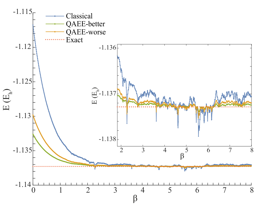
In this section, we present supplementary numerical results of the classical and quantum-assisted AFMC algorithms. A linear chain and a Hydrogen molecule are considered, and for both cases, the interatomic distance is . Taking the STO-3G basis, we take the Hartree-Fock state as CCTS (as it is commonly used), which has the fidelity of and with respect to the ground state of and , corresponding to an error of and in the ground state energy, respectively. For the quantum-assisted algorithm, we use two UCCSD trial states for , with a state fidelity of and , respectively, which correspond to an error of and ; for , we use a UCCSD trial state with a fidelity of and an error of . The phaseless approximation is used in the simulation to eliminate the sign problem.
The result of the energy of a molecule is shown in Fig. 5. As increases, all the three curves stabilise to approach the exact ground state, while the blue curve (representing the result from the classical algorithm) is observed to have a larger bias and variance than the two other curves (representing results from the quantum-assisted algorithm with different trial states), indicating that the quantum-assisted algorithm generates a better result. Similar results are observed for , as summarised in Table 5, which shows the error in the ground state energy. Compared with the results for VMC and fn-GFMC, we see the error from both the classical and quantum-assisted ph-AFMC algorithms is smaller, as is usually the case for classical algorithms; that’s because in AFMC, the walker state is a general Slater determinant close to the ground state and the local energy fluctuates around the actual energy. On the other hand, such a feature also makes AFMC more challenging to implement for both classical and quantum-assisted algorithms.
Appendix C Detailed derivation in amplitude estimation
C.1 The vacuum reference method
In this section we show the circuit in Fig. 2(b) can compute the real and imaginary parts of the amplitude .
In the circuit, the first Hadamard gate prepares the state and the following CNOT gates transform the state into
| (37) |
The first qubit is measured in the or basis, while all the other qubits are measured in state. Therefore, the circuit effectively measures the operator :
| (38) |
where refers to those CNOT gates before measurement. satisfies and , thus
| (39) |
C.2 The Hartree-Fork reference method
We can write the trial state as
| (42) |
where is a state orthogonal to and . So the amplitude to find is .
The circuit in Fig. 2(c) measures or . We take as the example. The circuit evaluates
| (43) |
As we assume is positive, is real, thus
| (45) |
Similarly we can find
| (46) |
thus
| (47) |