跳到论文正文
W Papers独立论文阅读器 arXiv:2205.14586 论文正文 计算阅读时间 · 0%
引用这篇论文根据当前论文元数据生成,正式投稿前建议核对。


License: CC BY-NC-ND 4.0
arXiv:2205.14586v1 [cs.SE] 29 May 2022
\checkfont

msam10 \correspondAritra Hazra, Department of Computer Science and Engineering, Indian Institute of Technology Kharagpur, Paschim Medinipur, West Bengal, India, PIN – 721302. E-mail: aritrah@cse.iitkgp.ac.in \pagerangeFormal Methods for Characterization and Analysis of Quality Specifications in Component-based Systems–

\makecorrespond

Formal Methods for Characterization and Analysis of Quality Specifications in Component-based Systems

Aritra Hazra
Department of Computer Science and Engineering
   Indian Institute of Technology Kharagpur    India
2000
Abstract

Component-based design paradigm is of paramount importance due to prolific growth in the complexity of modern-day systems. Since the components are developed primarily by multi-party vendors and often assembled to realize the overall system, it is an onus of the designer to certify both the functional and non-functional requirements of such systems. Several of the earlier works concentrated on formally analyzing the behavioral correctness, safety, security, reliability and robustness of such compositional systems. However, the assurance for quality measures of such systems is also considered as an important parameter for their acceptance. Formalization of quality measures is still at an immature state and often dictated by the user satisfaction. This paper presents a novel compositional framework for reliable quality analysis of component-based systems from the formal quality specifications of its constituent components. The proposed framework enables elegant and generic computation methods for quality attributes of various component-based system structures. In addition to this, we provide a formal query-driven quality assessment and design exploration framework which enables the designer to explore various component structures and operating setups and finally converge into better acceptable systems. A detailed case-study is presented over a component-based system structure to show the efficacy and practicality of our proposed framework.

keywords
Component-Based Systems, Specification, Quality, Reliability, Series-Parallel Composition.

1 Introduction

Component-based design engineering is of paramount importance across all engineering disciplines where complex systems can be obtained by assembling components as basic building blocks [13, 25, 27, 30]. Such paradigms are becoming prevalent due to increasing complexity of hardware and software systems and components requiring procurement from multi-party vendors for product completion. Components are design abstractions that ignore implementation details and are conceptualized formally using behavioral, interaction and execution models. These models are, then, hierarchically composed to build the overall system architecture where the formalism for the composite model is attributed from the notion of transfer functions, interfaces and contracts [1, 2, 6, 34]. Component-based engineering broadly involves model-based development of systems [33, 36], platform-based design methodologies [31] and developing software modules, supported by a large number of existing tools and standards, involving object-oriented languages (such as C++, System-C) and modeling languages (such as Stateflow/Statechart, UML, SysML) [5, 16, 17].

The computer scientists and researchers have responded to the challenge of designing complex systems adopting various formal methods and compositional algebra based frameworks [34, 35]. Typically, the component interactions and concurrency have been modeled formally using automated compositional reasoning and connector algebra [3, 4, 32]. With the wider adoption of such structured frameworks for system modeling, it also becomes a primary concern for the designers to ensure the correct operability of composite systems. Over the past few decades, model-based testing [37, 38] and model checking paradigms are explored to ensure the functional correctness, timing and safety behaviors [8, 9]. Additionally, several formal methods are proposed to enforce correct-by-construction approaches while designing system-level composite architectures [15, 29]. In recent times, the certification regime has also been extended towards formal assurance of the non-functional requirements as well, such as power [21, 22], reliability [14, 19, 20] and security [10, 18, 24], for component-based systems. Though the composition modeling is primarily formalized by the help of behavioral component models, formal component interactions and architectural properties, but there is a gap in modeling and assessment of system-level quality from the quality standards of its constituent components.

Quality measures of a system (often considered as a non-functional attribute) primarily reflects how perfectly an operation can be performed by the system and it is often attributed from the composed quality goals attained by its constituent components. It leads to the satisfaction of the users who are being serviced by the output of that system. A real-life example can be witnessed in case of video rendering (one can consider YouTube as an example) during the transmission/streaming where multiple levels of video quality can be produced. Typically, a high quality video input is being processed in multiple operating modes and the output video is produced in various quality levels depending on the bandwidth of the transmission and receiver channel. The two interesting non-functional behaviors in such a procedure is the reliability (or the availability) of the output video and also its quality parameters. The notion of reliability and availability in system design has been extensively studied [26]. However, at recent times, there is a growing need to incorporate the quality measures also into the main-stream formal system design process. The existing formalism for component-based rigorous system designs [34] do not consider into account quality attributes and associated specifications into their present modeling setup, hence the notion and formal treatment of quality measures in component-based systems are still remaining at a premature stage.

As per the best of our knowledge, there are very few works in formal system quality analysis. Some of the early works have subjectively quantified the notion of quality of systems and informally established the same by interaction of components and by following strict designing principles [7]. In embedded system design parlance, architectural quality assurance frameworks, leveraging naïve formal verification and model-based techniques, are formalized in [23, 28]. The notion of symbolic quality and its control was introduced in [11], where the authors propose an optimal quality schedule to ensure Quality-of-Service (QoS). On the same line, the work presented in [12] proposes a fine grain symbolic quality control method for multimedia applications using speed diagrams. The proposed methods takes as input an application software composed of actions, whose execution times are unknown increasing functions considering quality level parameters (considered as integers). The quality controller is able to compute adequate action schedules and choose pre-defined quality levels, in order to meet QoS requirements for a given platform. However, all these existing works do not provide the formal basis for designing and reasoning system involving component-level quality compositions; rather these methods invokes a quality manager to change action quality levels based on the knowledge of control constraints and finally computing a set of optimal schedules improving overall system performance.

Formal characterization of system quality has several deeper underpinnings in relation with the underlying system behavior. The choice of quality may have certain dependence with the system reliability, since some good quality component failure may degrade the overall quality of the system as well. So, formalizing the notions of quality should also incorporate the component-based system reliability formalism into its characterization. Existing literature provides several stand-alone techniques for calculating the reliability of systems based on symbolic/algebraic compositions of component-level reliability expressions from its given component structures [26]. However, there is a lack of effort in formally capturing quality measures for a design in similar terms, and thereby building a suitable framework to assess the compositional quality of component-based systems. This article is an enabler in this direction.

Refer to caption
Figure 1: The Overall Framework of Characterization and Assessment of Quality Specifications

Formally, we define the quality of a component as a set of random variables each associated with a probability value. We assume that for a given minimum input quality value/level, the corresponding minimum output quality value/level for any component is associated with a reliability value, which dictates its probability of successful execution without compromising the mentioned quality. The set of quality levels with different reliability values for a component arises due to a bound on limited execution time and cost of the component comprising the system [12]. Apart from the failure that can occur in a component structure, its operation can also be manually suspended by controlling it (for example, switching it off or executing it in a low functional/power modes) systematically. Such control of component suspension is very important at present context, considering the criticality of power, security and other performance criteria under restricted design setup. Clearly, a component has the output quality zero when its reliability is also zero (irrespective of input quality), meaning that failure is imminent, or its operation has been suspended (controlled). So, it is imperative to formulate algebra for component quality and reliability composition in order to reason about the quality of a system constructed hierarchically from set of component structures.

Given a set of formal quality and reliability specifications for a set of components, it is non-trivial to define the quality and reliability measures of the composite system structure. The composition is not similar to reliability analysis, since there is a choice here to maximize the overall quality during the compositional exploration considering the functional reliability of its constituent components (and their failures). This choice is complicated because there can be multiple ways during system execution to produce the range of quality expressions. For example, when several components, each having a set of quality specifications, are all connected in parallel, the overall quality measure of such a setup may be generated by – (i) computing the highest quality value/level among the operational components every time, (ii) assuming a pre-selected order among the operability of the constituent components, or (iii) reporting the quality from a fixed component (for simplicity) and the quality becomes zero when that component fails – thereby keeping the possibility for varied range of behavioral options. On the other hand, for series composition, the quality value is dictated by the series of components and becomes zero if any one of the components fails. Apart from such choices, the option to suspend/control the component execution in any operating mode brings inherent challenges in assessment of overall system quality attributes.

This work proposes novel methods for formal characterization and assessment of quality specifications for component-based systems that are built involving of series and parallel compositions of component structures at an architectural level. Figure 1 presents the overall flow (steps) of the work presented in this article. To start with, the component-level quality and reliability specifications (QRSpec) are drafted, which are then formally characterized into a set of component-level QRModel. Next, depending on the system structure, a generic series and parallel composition algebra is followed to formally compose these component models into a composite system-level QRModel. Now, the system level (architectural) QRSpec can also be reverse-synthesized, which may help in – (i) understanding the non-functional performance boundaries (and extremities) of the system under various component-level operating conditions, and (ii) performing a conformance check with respect to the given system configuration, in case the system specifications are known a priori, to compare and know the functional coverage of the system. However, QRSpec only defines an abstraction in terms of specifying the underlying detailed QRModel of the system. Many other interesting observations can be gleaned from QRModel that are not reflected directly through QRSpec, and these will be useful for the designers, who may want to explore various structures and combinations of available component to converge into the best possible system architecture. For that, the designer are given an option to formulate their queries over the system attributes systematically using a proposed structured query description language (SQDL), using which the information gets automatically extracted from the QRModel so that system-level quality and reliability (non-functional) assessments can be performed. In particular, the key contributions out of this work are:

  • •

    We define the specification formalism for component-level and system-level quality attributes.

  • •

    We introduce a uniform formal characterization of quality configurations for components and subsystems.

  • •

    We propose a novel series/parallel quality composition mechanism to hierarchically derive quality configurations for any given system architecture from its component-level quality models.

  • •

    We derive the (abstracted) system quality specification from the formal representation of system quality measures through reverse-synthesis to check for conformance and estimate coverage.

  • •

    We design a query-driven framework to aid designers for better system exploration and quality assessment.

  • •

    We provide a detailed case-study to show the efficacy and practicality of our proposed formal framework.

The rest of the paper is organized as follows11 1 Sections are also highlighted in Figure 1 to provide a meaningful organization to this article.. Section 2 describes the formal modeling of component-based systems and the notion of quality specifications for the components and subsystems. Section 3 presents the formal characterization of quality measures from quality specifications. Section 4 introduces the primitive composition techniques for series and parallel system structures and formulate generic composition principles for systems. Section 5 elaborates on the synthesis of quality specifications from formal models and conformance checking part. Section 6 proposes the query processing and analysis platform for system-level assessment and design exploration. Section 7 illustrates our proposed framework empirically over few case-studies of composite structures. Finally, Section 8 concludes the work presented in this article.

2 Formal Model and Specification

Component-based design approaches follow the development of an overall system starting from unit-level component structures and laying their specifications. In this section, we first formalize the description of such component-based systems and the notion of formal quality specifications.

2.1 Component-based Systems

Several components may be connected with each other in series and parallel structures to form a system. Formally, such a component-based system, Υ\Upsilon, can be expressed as,

Υ=⟨ℐ,𝒪,𝒞,𝒱,ℰ,ℒ⟩,where:\Upsilon=\langle\mathcal{I},\mathcal{O},\mathcal{C},\mathcal{V},\mathcal{E},\mathcal{L}\rangle,\ \ \mbox{where:}
  • •

    ℐ={I1,I2,…,Iu}\mathcal{I}=\{I_{1},I_{2},\ldots,I_{u}\} denotes the set of uu input nodes of the system.

  • •

    𝒪={O1,O2,…,Ov}\mathcal{O}=\{O_{1},O_{2},\ldots,O_{v}\} denotes the set of vv output nodes of the system.

  • •

    𝒞={C1,C2,…,Cn}\mathcal{C}=\{C_{1},C_{2},\ldots,C_{n}\} denotes the set of nn components of the system, where each component CiC_{i} (with a single input and single output) has their own non-functional specification, 𝒫i\mathcal{P}_{i} (defined in next subsection).

  • •

    𝒱={V1,V2,…,Vz}\mathcal{V}=\{V_{1},V_{2},\ldots,V_{z}\} denotes the set of zz vertices (z≥nz\geq n).

  • •

    ℰ⊆(ℐ∪𝒱)×(𝒱∪𝒪)\mathcal{E}\subseteq(\mathcal{I}\cup\mathcal{V})\times(\mathcal{V}\cup\mathcal{O}) denotes the set of edges representing the connectors among the vertices including the input/output nodes of the system.

  • •

    ℒ:𝒱→𝒞\mathcal{L}:\mathcal{V}\rightarrow\mathcal{C} is a function that labels each vertices with a component. There may be multiple vertices labeled with a same component indicating that the component is used in multiple places in the system.

The following example of a component-based system illustrates the above mentioned formalism in details.

Example 1

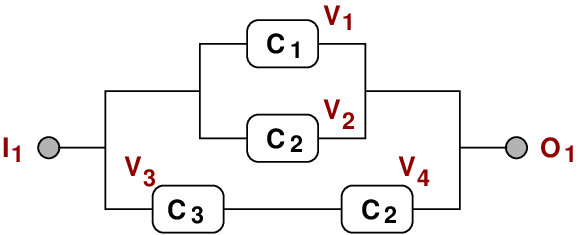
Consider the example of a series/parallel component-based system, Υs​p\Upsilon_{sp}, given in Figure 2. Here, 𝒞={C1,C2,C3}\mathcal{C}=\{C_{1},C_{2},C_{3}\}, ℐ={I1}\mathcal{I}=\{I_{1}\} and 𝒪={O1}\mathcal{O}=\{O_{1}\}. The overall system architecture can be represented using a directed acyclic graph with the set of vertices, 𝒱={V1,V2,V3,V4}\mathcal{V}=\{V_{1},V_{2},V_{3},V_{4}\}, and the set of edges, ℰ={(I1,V1);(I1,V2);(I1,V3);(V3,V4);\mathcal{E}=\{(I_{1},V_{1});(I_{1},V_{2});(I_{1},V_{3});(V_{3},V_{4}); (V1,O1);(V2,O1);(V4,O1)}(V_{1},O_{1});(V_{2},O_{1});(V_{4},O_{1})\}. Moreover, the vertices are labeled using three components forming the system architecture as, ℒ⁡(V1)=C1\mathcal{L}(V_{1})=C_{1}, ℒ⁡(V2)=C2\mathcal{L}(V_{2})=C_{2}, ℒ⁡(V3)=C3\mathcal{L}(V_{3})=C_{3}, and ℒ⁡(V4)=C2\mathcal{L}(V_{4})=C_{2}.

Refer to caption
Figure 2: Component-based System Structure, Υs​p\Upsilon_{sp}, having Series and Parallel Component Organization

□\Box

A few pertinent points to note here are as follows.

  • •

    The series and parallel system structure is useful in designing many safety-critical systems where the same input-output design functionality can get realized via redundant parallel paths in order to tolerate some intermediate component failures. Typically, the functionalities from a set of parallel executions/paths are converged using a voting mechanism (choosing consistent outcomes from mm-out-of-nn paths). For example, in Figure 2, three parallel paths, i.e. via C1C_{1}, via C2C_{2}, or via C3−C2C_{3}-C_{2}, may yield the same input-output functionality, though their way of implementation may vary (due to procurement of each component from different sources). From a functional perspective, we may vote and produce output by taking consistent outcomes from 22-out-of-33 paths22 2 To reduce clutter and without loss of generality, we have not explicitly shown the voting component in the system structure.. However, whenever the parallel paths converge, the overall output quality may come from either choosing the maximum quality across all paths, or choosing quality values from some pre-defined ordering of paths (we discuss this in details in the following sections). Further, we assume that the voting component is fully reliable and do not degrade the quality parameters while bypassing through it. In practical cases, we can take quality and reliability specifications also for the voter and treat it like another component being placed in series whenever a set of parallel paths converge.

  • •

    When the same component is placed in multiple positions of the overall system, it indicates different instantiation (in case of hardware systems) or different invocations (in case of software systems) of the same object (defined once). So, going by this analogy, in Figure 2, where there is two installation of same component C2C_{2}, if C2C_{2} fails, then the operating probability of C2C_{2} becomes 00 and hence two paths (I1→V3→V4→O1I_{1}\rightarrow V_{3}\rightarrow V_{4}\rightarrow O_{1} and I1→V2→O1I_{1}\rightarrow V_{2}\rightarrow O_{1}) fail together (out of three possible) from input to output.

  • •

    On the other hand, whenever there is a need to place a duplicate but identical component in the other places, a different component name (with same specifications though) needs to used in every other constellations. For example, it may be the case in Figure 2 that C1C_{1} and C3C_{3} are identical components in terms of their functionality, but separately defined.

  • •

    In practical conditions, sometimes to save power and other design overhead, some redundant components may be suspended or switched off (usually controlled by the designer). Component failure and suspension are different, because in first case, if the component has an operating reliability of rr, then it has its failure probability of (1−r)(1-r); whereas the latter makes the component to bypass assuming a reliability of 11 for the suspended component. For example, in Figure 2, if we suspend C3C_{3}, then the path via I1→V3→V4→O1I_{1}\rightarrow V_{3}\rightarrow V_{4}\rightarrow O_{1} is blocked due to suspension of C3C_{3}, but C3C_{3} will have reliability as 11.

2.2 Quality and Reliability Specifications

Typically, in component-based system design, the quality and reliability attributes, often known as non-functional requirements, are laid from an architectural level of the system and are analyzed over the system structures. We term such non-functional quality and reliability specifications as QRSpec. First, let us formally define such a high-level QRSpec of a component as well as an overall system.

2.2.1 Component-level Specifications

Every unit-level component within a system operates in multiple modes (each mode having a given operational reliability value between [0,1][0,1]) provided it does not undergo any failure33 3 We treat component failure also as an operational mode with reliability being 00.. Now, corresponding to every quality level of the input for a component, it produces the output in some defined quality levels depending on its mode of operation. Formally, we represent the QRSpec for a unit-level component, CiC_{i}, as:

𝒫i=⟨{Ci},Mi,Zi,QiI,QiO⟩,where:\mathcal{P}_{i}=\langle\{C_{i}\},M_{i},Z_{i},Q_{i}^{I},Q_{i}^{O}\rangle,\quad\text{where:}
  • •

    {Ci}\{C_{i}\} is the participating component.

  • •

    Mi={mi0,mi1,mi2,…,midi}M_{i}=\{m_{i}^{0},m_{i}^{1},m_{i}^{2},\ldots,m_{i}^{d_{i}}\}, denotes the set of (di+1)(d_{i}+1) operational modes of CiC_{i} including mi0m_{i}^{0} as the failure mode (di∈ℕd_{i}\in\mathbb{N}).

  • •

    Zi:Mi→ℝ[0,1]Z_{i}:M_{i}\rightarrow\mathbb{R}^{[0,1]}, is a function that associates a reliability value (within [0,1][0,1]) to each operational mode of the component. Here, Zi​(mi0)=0Z_{i}(m_{i}^{0})=0 and ∀k⁡(1≤k≤di),Zi​(mik)>0\forall k\ (1\leq k\leq d_{i}),\ Z_{i}(m_{i}^{k})>0.

  • •

    QiI={qi1,qi2,…,qili}Q_{i}^{I}=\{q_{i}^{1},q_{i}^{2},\ldots,q_{i}^{l_{i}}\}, denotes the set of lil_{i} non-negative input quality values (or levels), where ∀j⁡(1≤j<li),qij∈ℝ+\forall j\ (1\leq j<l_{i}),\ q_{i}^{j}\in\mathbb{R}^{+} and qij>qij+1q_{i}^{j}>q_{i}^{j+1}.

  • •

    QiO:Mi×QiI→ℝ+Q_{i}^{O}:M_{i}\times Q_{i}^{I}\rightarrow\mathbb{R}^{+}, is a function that maps each input quality level to an output quality (a non-negative real number) corresponding to every operational modes.
    It may be noted that, ∀k⁡(1≤k≤di),∀j⁡(1≤j≤li),QiO​(mik,qij)≤qij\forall k\ (1\leq k\leq d_{i}),\ \forall j\ (1\leq j\leq l_{i}),\ Q_{i}^{O}(m_{i}^{k},q_{i}^{j})\leq q_{i}^{j} and QiO​(mi0,qij)=0Q_{i}^{O}(m_{i}^{0},q_{i}^{j})=0, as mi0m_{i}^{0} indicates the mode where CiC_{i} failed completely. Moreover, if the input quality (qq) falls below qiliq_{i}^{l_{i}}, then the output quality becomes zero, i.e. QiO​(mik,q)=0Q_{i}^{O}(m_{i}^{k},q)=0, when q<qiliq<q_{i}^{l_{i}}.

Here, every operating mode for a component has a reliability and can produces different quality output values based on given input quality ranges. The following example illustrates the component QRSpec formalism.

Example 2

Let the QRSpec for a component, C1C_{1}, is given as, 𝒫1=⟨M1,Z1,Q1I,Q1O⟩\mathcal{P}_{1}=\langle M_{1},Z_{1},Q_{1}^{I},Q_{1}^{O}\rangle, where:

  • •

    C1C_{1} operates in two operational modes along with a permanent failure mode. Therefore, M1={m10,m11,m12}M_{1}=\{m_{1}^{0},m_{1}^{1},m_{1}^{2}\}.

  • •

    The operational reliability values are, Z1​(m11)=0.8Z_{1}(m_{1}^{1})=0.8, Z1​(m12)=0.7Z_{1}(m_{1}^{2})=0.7, and Z1​(m10)=0Z_{1}(m_{1}^{0})=0.

  • •

    The input quality levels are specified as, Q1I={50,30,20}Q_{1}^{I}=\{50,30,20\}.

  • •

    The corresponding output quality values are, Q1O​(m11,50)=40Q_{1}^{O}(m_{1}^{1},50)=40, Q1O​(m11,30)=25Q_{1}^{O}(m_{1}^{1},30)=25, Q1O​(m11,20)=10Q_{1}^{O}(m_{1}^{1},20)=10 and Q1O​(m12,50)=35Q_{1}^{O}(m_{1}^{2},50)=35, Q1O​(m12,30)=25Q_{1}^{O}(m_{1}^{2},30)=25, Q1O​(m12,20)=10Q_{1}^{O}(m_{1}^{2},20)=10.
    It intuitively means that, the output quality levels maintained by C1C_{1} at mode m11m_{1}^{1} are at least 4040, 2525 and 1010 when the input quality value is at least 5050, within [30,50)[30,50) and within [10,30)[10,30), respectively.
    Implicitly, for any q∈ℝ+q\in\mathbb{R}^{+}, Q1O​(m10,q)=0Q_{1}^{O}(m_{1}^{0},q)=0 and when q<20q<20, Q1O​(m11,q)=0Q_{1}^{O}(m_{1}^{1},q)=0 and Q1O​(m12,q)=0Q_{1}^{O}(m_{1}^{2},q)=0.

Similarly, let the quality specification for C2C_{2} is given as, 𝒫2=⟨M2,Z2,Q2I,Q2O⟩\mathcal{P}_{2}=\langle M_{2},Z_{2},Q_{2}^{I},Q_{2}^{O}\rangle, where: M2={m20,m21}M_{2}=\{m_{2}^{0},m_{2}^{1}\}; Z2​(m21)=0.95Z_{2}(m_{2}^{1})=0.95 and Z2​(m20)=0Z_{2}(m_{2}^{0})=0; Q2I={40,10}Q_{2}^{I}=\{40,10\}; Q1O​(m21,40)=30Q_{1}^{O}(m_{2}^{1},40)=30 and Q2O​(m21,10)=10Q_{2}^{O}(m_{2}^{1},10)=10.

Also, let the quality specification for C3C_{3}, is given as, 𝒫3=⟨M3,Z3,Q3I,Q3O⟩\mathcal{P}_{3}=\langle M_{3},Z_{3},Q_{3}^{I},Q_{3}^{O}\rangle, where: M3={m30,m31,m32}M_{3}=\{m_{3}^{0},m_{3}^{1},m_{3}^{2}\}; Z3​(m31)=0.9Z_{3}(m_{3}^{1})=0.9, Z3​(m32)=0.8Z_{3}(m_{3}^{2})=0.8 and Z3​(m30)=0Z_{3}(m_{3}^{0})=0; Q3I={50,20,10}Q_{3}^{I}=\{50,20,10\}; Q3O​(m31,50)=45Q_{3}^{O}(m_{3}^{1},50)=45, Q3O​(m31,20)=20Q_{3}^{O}(m_{3}^{1},20)=20, Q3O​(m31,10)=5Q_{3}^{O}(m_{3}^{1},10)=5 and Q3O​(m32,50)=40Q_{3}^{O}(m_{3}^{2},50)=40, Q3O​(m32,20)=15Q_{3}^{O}(m_{3}^{2},20)=15, Q3O​(m32,10)=5Q_{3}^{O}(m_{3}^{2},10)=5. □\Box

2.2.2 System-level Specifications

A system architecture is built using a set of inter-connected components which are glued with each other in a series/parallel manner. Formally, we define the QRSpec for an overall system, Υ\Upsilon, as44 4 It may be noted that, component-level QRSpec can also be viewed as a system-level QRSpec where CΥ={Ci}C_{\Upsilon}=\{C_{i}\}, i.e., the system, Υ\Upsilon, comprises of a single component, CiC_{i}. Hence, from the next section onwards, we do not differentiate between component and system as such, since their formal modeling and treatment remains uniform.:

𝒫Υ=⟨CΥ,MΥ,ZΥ,QΥI,QΥO⟩,where:\mathcal{P}_{\Upsilon}=\langle C_{\Upsilon},M_{\Upsilon},Z_{\Upsilon},Q_{\Upsilon}^{I},Q_{\Upsilon}^{O}\rangle,\quad\text{where:}
  • •

    CΥ={C1,C2,…,Cn}C_{\Upsilon}=\{C_{1},C_{2},\ldots,C_{n}\}, is the set of nn components used to form the system, Υ\Upsilon.
    The quality specification for each component, CiC_{i} (1≤i≤n1\leq i\leq n), is denoted by, 𝒫i=⟨Mi,Zi,QiI,QiO⟩\mathcal{P}_{i}=\langle M_{i},Z_{i},Q_{i}^{I},Q_{i}^{O}\rangle.

  • •

    MΥ=(M1×M2×⋯×Mn)M_{\Upsilon}=(M_{1}\times M_{2}\times\cdots\times M_{n}), denotes the set of dΥd_{\Upsilon} operational modes of Υ\Upsilon, where each mode is an nn-tuple and hence dΥ=∏i=1n(di+1)d_{\Upsilon}=\prod_{i=1}^{n}(d_{i}+1).

  • •

    ZΥ:MΥ→ℝ[0,1]Z_{\Upsilon}:M_{\Upsilon}\rightarrow\mathbb{R}^{[0,1]}, is a function that associates a reliability value (within [0,1][0,1]) to each operational mode of the system.

  • •

    QΥI⊆⋃i=1nQiIQ_{\Upsilon}^{I}\subseteq\bigcup\limits_{i=1}^{n}Q_{i}^{I}, denotes the set of non-negative input quality values (levels);

  • •

    QΥO:MΥ×QΥI→ℝ+Q_{\Upsilon}^{O}:M_{\Upsilon}\times Q_{\Upsilon}^{I}\rightarrow\mathbb{R}^{+}, is a function that maps each input quality level to an output quality (a non-negative real number) for every operational modes.

The following example demonstrates the QRSpec of two elementary systems, ΥP\Upsilon_{P} and ΥS\Upsilon_{S}, each having two components connected simply in parallel and series, respectively.

Example 3

First, let us consider another elementary system, ΥS\Upsilon_{S}, comprised of two components, C2C_{2} and C3C_{3} (as introduced in Example 2), where C2C_{2} is connected with C3C_{3} in series (refer to Figure 3(a)). Now, the QRSpec for ΥS\Upsilon_{S} is given as, 𝒫ΥS=⟨CΥS,MΥS,ZΥS,QΥSI,QΥSO⟩\mathcal{P}_{\Upsilon_{S}}=\langle C_{\Upsilon_{S}},M_{\Upsilon_{S}},Z_{\Upsilon_{S}},Q_{\Upsilon_{S}}^{I},Q_{\Upsilon_{S}}^{O}\rangle, where:

  • •

    The participating components are, CΥS={C2,C3}C_{\Upsilon_{S}}=\{C_{2},C_{3}\} with QRSpec, 𝒫2\mathcal{P}_{2} and 𝒫3\mathcal{P}_{3}, respectively.

  • •

    The three operational modes of ΥS\Upsilon_{S} are, MΥS={mΥS0,mΥS1,mΥS2}M_{\Upsilon_{S}}=\{m_{\Upsilon_{S}}^{0},m_{\Upsilon_{S}}^{1},m_{\Upsilon_{S}}^{2}\}, where:

    mΥS0≡(m30,m20)≡(m30,m21)≡(m31,m20)≡(m32,m20),mΥS1≡(m31,m21),mΥS2≡(m32,m21).m_{\Upsilon_{S}}^{0}\equiv(m_{3}^{0},m_{2}^{0})\equiv(m_{3}^{0},m_{2}^{1})\equiv(m_{3}^{1},m_{2}^{0})\equiv(m_{3}^{2},m_{2}^{0}),\quad m_{\Upsilon_{S}}^{1}\equiv(m_{3}^{1},m_{2}^{1}),\quad m_{\Upsilon_{S}}^{2}\equiv(m_{3}^{2},m_{2}^{1}).

    Effectively, only two modes, (m31,m21)(m_{3}^{1},m_{2}^{1}) and (m32,m21)(m_{3}^{2},m_{2}^{1}), are non-failure (operating) modes and the rest are all failure modes.

  • •

    Since C2C_{2} and C3C_{3} are in series, so the reliability corresponding to every mode of MΥSM_{\Upsilon_{S}} is be computed as, ZΥS((m3j,m2k))=Z1(m3j).Z2(m2k)(0≤j≤2 and 0≤k≤1)Z_{\Upsilon_{S}}\big((m_{3}^{j},m_{2}^{k})\big)=Z_{1}(m_{3}^{j}).Z_{2}(m_{2}^{k})\ (0\leq j\leq 2\text{ and }0\leq k\leq 1) and shown in Table 2.

  • •

    The input quality levels are, QΥSI={50,20}Q_{\Upsilon_{S}}^{I}=\{50,20\} (due to series connected components).

  • •

    The output quality value function (QΥSOQ_{\Upsilon_{S}}^{O}), with respect to the input quality values/levels for every operational mode of ΥS\Upsilon_{S} is also given in Table 255 5 To intuitively explain (detailed methodology is presented later) the last row of Table 2, note that the system mode, mΥS2≡(m32,m21)m_{\Upsilon_{S}}^{2}\equiv(m_{3}^{2},m_{2}^{1}), is dictated by the operating modes of C3C_{3} and C2C_{2}. The output quality values corresponding to input quality level at least 5050 and within [20,50)[20,50) can be computed as, QΥSO​((m32,m21),50)=Q2O​(m21,Q3O​(m32,50))=Q2O​(m21,40)=30Q_{\Upsilon_{S}}^{O}\big((m_{3}^{2},m_{2}^{1}),50\big)=Q_{2}^{O}\big(m_{2}^{1},Q_{3}^{O}(m_{3}^{2},50)\big)=Q_{2}^{O}\big(m_{2}^{1},40\big)=30, and similarly, QΥSO​((m32,m21),20)=Q2O​(m21,Q3O​(m32,20))=Q2O​(m21,15)=Q2O​(m21,10)=10Q_{\Upsilon_{S}}^{O}\big((m_{3}^{2},m_{2}^{1}),20\big)=Q_{2}^{O}\big(m_{2}^{1},Q_{3}^{O}(m_{3}^{2},20)\big)=Q_{2}^{O}\big(m_{2}^{1},15\big)=Q_{2}^{O}\big(m_{2}^{1},10\big)=10 (since C2C_{2} is placed after C3C_{3} in series)..

Refer to caption
Figure 3: (a) 2-Component Series System, ΥS\Upsilon_{S}   (b) 2-Component Parallel System, ΥP\Upsilon_{P}
System Mode Reliability Input Quality Output Quality
mΥS0≡(m30,m20)m_{\Upsilon_{S}}^{0}\equiv(m_{3}^{0},m_{2}^{0}) 0.0000.000 ⟨0⟩\langle 0\rangle ⟨0⟩\langle 0\rangle
mΥS0≡(m30,m21)m_{\Upsilon_{S}}^{0}\equiv(m_{3}^{0},m_{2}^{1}) 0.0000.000 ⟨0⟩\langle 0\rangle ⟨0⟩\langle 0\rangle
mΥS0≡(m31,m20)m_{\Upsilon_{S}}^{0}\equiv(m_{3}^{1},m_{2}^{0}) 0.0000.000 ⟨0⟩\langle 0\rangle ⟨0⟩\langle 0\rangle
mΥS1≡(m31,m21)m_{\Upsilon_{S}}^{1}\equiv(m_{3}^{1},m_{2}^{1}) 0.8550.855 ⟨50,20⟩\langle 50,20\rangle ⟨30,10⟩\langle 30,10\rangle
mΥS0≡(m32,m20)m_{\Upsilon_{S}}^{0}\equiv(m_{3}^{2},m_{2}^{0}) 0.0000.000 ⟨0⟩\langle 0\rangle ⟨0⟩\langle 0\rangle
mΥS2≡(m32,m21)m_{\Upsilon_{S}}^{2}\equiv(m_{3}^{2},m_{2}^{1}) 0.7600.760 ⟨50,20⟩\langle 50,20\rangle ⟨30,10⟩\langle 30,10\rangle
Table 1: Mode-wise Reliability and Quality Values for ΥS\Upsilon_{S}
System Mode Reliability Input Quality Output Quality
mΥP0≡(m10,m20)m_{\Upsilon_{P}}^{0}\equiv(m_{1}^{0},m_{2}^{0}) 0.0000.000 ⟨0⟩\langle 0\rangle ⟨0⟩\langle 0\rangle
mΥP1≡(m10,m21)m_{\Upsilon_{P}}^{1}\equiv(m_{1}^{0},m_{2}^{1}) 0.9500.950 ⟨40,10⟩\langle 40,10\rangle ⟨30,10⟩\langle 30,10\rangle
mΥP2≡(m11,m20)m_{\Upsilon_{P}}^{2}\equiv(m_{1}^{1},m_{2}^{0}) 0.8000.800 ⟨50,30,20⟩\langle 50,30,20\rangle ⟨40,25,10⟩\langle 40,25,10\rangle
mΥP3≡(m11,m21)m_{\Upsilon_{P}}^{3}\equiv(m_{1}^{1},m_{2}^{1}) 0.9900.990 ⟨50,40,30,10⟩\langle 50,40,30,10\rangle ⟨40,30,25,10⟩\langle 40,30,25,10\rangle
mΥP4≡(m12,m20)m_{\Upsilon_{P}}^{4}\equiv(m_{1}^{2},m_{2}^{0}) 0.7000.700 ⟨50,30,20⟩\langle 50,30,20\rangle ⟨35,25,10⟩\langle 35,25,10\rangle
mΥP5≡(m12,m21)m_{\Upsilon_{P}}^{5}\equiv(m_{1}^{2},m_{2}^{1}) 0.9850.985 ⟨50,40,30,10⟩\langle 50,40,30,10\rangle ⟨35,30,25,10⟩\langle 35,30,25,10\rangle
Table 2: Mode-wise Reliability and Quality Values for ΥP\Upsilon_{P}

Now, let us consider an elementary system, ΥP\Upsilon_{P}, comprised of two components, C1C_{1} and C2C_{2} (as introduced in Example 2), where C1C_{1} is connected with C2C_{2} in parallel (refer to Figure 3(b)). Now, the QRSpec for ΥP\Upsilon_{P} is given as, 𝒫ΥP=⟨CΥP,MΥP,ZΥP,QΥPI,QΥPO⟩\mathcal{P}_{\Upsilon_{P}}=\langle C_{\Upsilon_{P}},M_{\Upsilon_{P}},Z_{\Upsilon_{P}},Q_{\Upsilon_{P}}^{I},Q_{\Upsilon_{P}}^{O}\rangle, where:

  • •

    The participating components are, CΥP={C1,C2}C_{\Upsilon_{P}}=\{C_{1},C_{2}\} with QRSpec, 𝒫1\mathcal{P}_{1} and 𝒫2\mathcal{P}_{2}, respectively.

  • •

    The six operational modes of ΥP\Upsilon_{P} are, MΥP={mΥP0,mΥP1,mΥP2,mΥP3,mΥP4,mΥP5}M_{\Upsilon_{P}}=\{m_{\Upsilon_{P}}^{0},m_{\Upsilon_{P}}^{1},m_{\Upsilon_{P}}^{2},m_{\Upsilon_{P}}^{3},m_{\Upsilon_{P}}^{4},m_{\Upsilon_{P}}^{5}\}, where:

    mΥP0≡(m10,m20),mΥP1≡(m10,m21),mΥP2≡(m11,m20),mΥP3≡(m11,m21),mΥP4≡(m12,m20),mΥP5≡(m12,m21).m_{\Upsilon_{P}}^{0}\equiv(m_{1}^{0},m_{2}^{0}),\ m_{\Upsilon_{P}}^{1}\equiv(m_{1}^{0},m_{2}^{1}),\ m_{\Upsilon_{P}}^{2}\equiv(m_{1}^{1},m_{2}^{0}),\ m_{\Upsilon_{P}}^{3}\equiv(m_{1}^{1},m_{2}^{1}),\ m_{\Upsilon_{P}}^{4}\equiv(m_{1}^{2},m_{2}^{0}),\ m_{\Upsilon_{P}}^{5}\equiv(m_{1}^{2},m_{2}^{1}).
  • •

    Since C1C_{1} and C2C_{2} are in parallel, so the reliability corresponding to every mode of MΥPM_{\Upsilon_{P}} is be computed as, ZΥP((m1j,m2k))=[1−(1−Z1(m1j)).(1−Z2(m2k))](0≤j≤2 and 0≤k≤1)Z_{\Upsilon_{P}}\big((m_{1}^{j},m_{2}^{k})\big)=\Big[1-\big(1-Z_{1}(m_{1}^{j})\big).\big(1-Z_{2}(m_{2}^{k})\big)\Big]\ (0\leq j\leq 2\text{ and }0\leq k\leq 1) and shown in Table 2.

  • •

    The input quality levels are, QΥPI={50,40,30,20,10}Q_{\Upsilon_{P}}^{I}=\{50,40,30,20,10\} (due to parallel connected components).

  • •

    The output quality value function (QΥPOQ_{\Upsilon_{P}}^{O}), with respect to the input quality values/levels for every operational mode of ΥP\Upsilon_{P} is also given in Table 266 6 To intuitively explain (detailed methodology is presented later) the last row of Table 2, note that the system mode, mΥP5≡(m12,m21)m_{\Upsilon_{P}}^{5}\equiv(m_{1}^{2},m_{2}^{1}), is dictated by the operating modes of C1C_{1} and C2C_{2}. The (best possible) output quality value with respect to input quality level at least 4040 can be computed as, QΥPO​((m12,m21),40)=𝙼𝙰𝚇⁡[Q1O​(m12,40),Q2O​(m21,40)]=𝙼𝙰𝚇⁡[Q1O​(m12,30),Q2O​(m21,40)]=𝙼𝙰𝚇⁡[25,30]=30Q_{\Upsilon_{P}}^{O}\big((m_{1}^{2},m_{2}^{1}),40\big)={\tt MAX}[Q_{1}^{O}(m_{1}^{2},40),Q_{2}^{O}(m_{2}^{1},40)]={\tt MAX}[Q_{1}^{O}(m_{1}^{2},30),Q_{2}^{O}(m_{2}^{1},40)]={\tt MAX}[25,30]=30. Similarly, we can also find all the (best possible) output quality values, 3535, 3030, 2525 and 1010 for the corresponding input quality values, which are at least 5050, within [40,50)[40,50), within [30,40)[30,40) and within [10,30)[10,30), respectively.. □\Box

It is worthy to note here is that, the architectural QRSpec of a system derives its operating modes and quality-reliability attributes with respect to component failures as well as component suspensions. Though the above example only deals with component failures (not provisionize component suspensions), however as pointed at the end of Section 2.1 (and also in Section 1), the designer may explore various quality attributes of a system also involving suspended components. Exploration of such orchestrations in component behaviors needs a generic compositional framework through which one can automatically derive out the system-level QRSpec from the QRSpec of its component modules involving both failure and suspended components. In subsequent sections, we present the generic procedures to formally derive system-level QRSpec from component QRSpec.

3 Formal Characterization of Quality Configurations

In this section, we present a formal characterization of the system-level quality measures under various operating configurations of its constituent components as state transition models, also termed as QRModel, which enables further compositional interpretation of the QRSpec. Formally, we characterize the quality measure under different operating configurations of a subsystem, Υ\Upsilon (having one or more components), with the QRSpec, 𝒫Υ=⟨CΥ,MΥ,ZΥ,QΥI,QΥO⟩\mathcal{P}_{\Upsilon}=\langle C_{\Upsilon},M_{\Upsilon},Z_{\Upsilon},Q_{\Upsilon}^{I},Q_{\Upsilon}^{O}\rangle, in terms of the following QRModel as,

𝒬Υ=⟨CΥ,QΥI,RΥ,SΥ,sΥ1,ΓΥ,QΥO,TΥ,𝙴𝚡𝚙𝚛Υ⟩,where:\mathcal{Q}_{\Upsilon}=\langle C_{\Upsilon},Q_{\Upsilon}^{I},R_{\Upsilon},S_{\Upsilon},s_{\Upsilon}^{1},\Gamma_{\Upsilon},Q_{\Upsilon}^{O},T_{\Upsilon},{\tt Expr}_{\Upsilon}\rangle,\quad\text{where:}
  • •

    CΥ={C1,C2,…,Cn}C_{\Upsilon}=\{C_{1},C_{2},\ldots,C_{n}\} is the ordered set of nn participating components in the system, Υ\Upsilon.

  • •

    QΥI={qΥ1,qΥ2,…,qΥlΥ}Q_{\Upsilon}^{I}=\{q_{\Upsilon}^{1},q_{\Upsilon}^{2},\ldots,q_{\Upsilon}^{l_{\Upsilon}}\}, denotes the set of lΥl_{\Upsilon} non-negative input quality values (or levels), where ∀j⁡(1≤j<lΥ),qΥj∈ℝ+\forall j\ (1\leq j<l_{\Upsilon}),\ q_{\Upsilon}^{j}\in\mathbb{R}^{+} and qΥj>qΥj+1q_{\Upsilon}^{j}>q_{\Upsilon}^{j+1}.

  • •

    RΥ={rΥ,1,rΥ,2,…,rΥ,eΥ}R_{\Upsilon}=\{r_{\Upsilon,1},r_{\Upsilon,2},\ldots,r_{\Upsilon,e_{\Upsilon}}\} is the set of eΥ(=∑i=1ndi)e_{\Upsilon}(=\sum_{i=1}^{n}d_{i}) symbolic reliability variables, such that each rΥ,kr_{\Upsilon,k}, corresponding to the operating mode mytm_{y}^{t} of CyC_{y}, has the reliability value of Zy​(myt)Z_{y}(m_{y}^{t}), where 1≤∑i=1y−1di<k≤∑i=1ydi≤eΥ1\leq\sum_{i=1}^{y-1}d_{i}<k\leq\sum_{i=1}^{y}d_{i}\leq e_{\Upsilon} and t=k−∑i=1y−1dit=k-\sum_{i=1}^{y-1}d_{i}.

  • •

    SΥ={sΥ1,sΥ2,…,sΥnΥ}S_{\Upsilon}=\{s_{\Upsilon}^{1},s_{\Upsilon}^{2},\ldots,s_{\Upsilon}^{n_{\Upsilon}}\} is the set of nΥn_{\Upsilon} operational states characterizing the quality measures. Here, nΥ=∏i=1n(2di+1−1)n_{\Upsilon}=\prod_{i=1}^{n}(2^{d_{i}+1}-1), where each CiC_{i} can operate in did_{i} number of modes (1≤i≤n1\leq i\leq n).

  • •

    sΥ1∈SΥs_{\Upsilon}^{1}\in S_{\Upsilon} is the start/initial operating state.

  • •

    ΓΥ:SΥ→{𝟷,𝟶,𝚇,𝚈}eΥ\Gamma_{\Upsilon}:S_{\Upsilon}\rightarrow\{{\tt 1,0,X,Y}\}^{e_{\Upsilon}} denotes the eΥe_{\Upsilon}-length configuration function of a state corresponding to dΥd_{\Upsilon} operational modes in MΥM_{\Upsilon} (excluding failure mode, mΥ0∈MΥm_{\Upsilon}^{0}\in M_{\Upsilon}, which can be expressed as the state having all 00’s in the eΥe_{\Upsilon}-length configuration). Here, eΥ=∑i=1ndie_{\Upsilon}=\sum_{i=1}^{n}d_{i}, where did_{i} is the number of operating modes (excluding the failure mode) of CiC_{i} (1≤i≤n1\leq i\leq n). Typically, CiC_{i} shall execute in the operating mode, mijm_{i}^{j}, when all modes mik​(1≤k<j≤di)m_{i}^{k}\ (1\leq k<j\leq d_{i}) have failed.

    For a state, sΥj∈SΥs_{\Upsilon}^{j}\in S_{\Upsilon}, ΓΥ​(sΥj)​[k]∈{𝟷,𝟶,𝚇,𝚈}\Gamma_{\Upsilon}(s_{\Upsilon}^{j})[k]\in\{{\tt 1,0,X,Y}\} and ΓΥ(sΥj)[k..k′]∈{𝟷,𝟶,𝚇,𝚈}(k′−k+1)\Gamma_{\Upsilon}(s_{\Upsilon}^{j})[k..k^{\prime}]\in\{{\tt 1,0,X,Y}\}^{(k^{\prime}-k+1)} (1≤k<k′≤eΥ1\leq k<k^{\prime}\leq e_{\Upsilon}) represent the kt​hk^{th} and kk-to-k′k^{\prime} configuration location(s) of sΥjs_{\Upsilon}^{j}, respectively. Formally,

    ΓΥ​(sΥj)​[k]={𝟷,indicating Cy is operating in mode myt 𝟶,indicating Cy is has failed in mode myt𝚇,indicating Cy is not availing mode myt𝚈,indicating Cy has suspended mode myt​where ​1≤∑i=1y−1di<k≤∑i=1ydi≤eΥ​ and ​t=k−∑i=1y−1di\Gamma_{\Upsilon}(s_{\Upsilon}^{j})[k]=\left\{\begin{array}[]{rl}{\tt 1},&\mbox{indicating $C_{y}$ is operating in mode $m_{y}^{t}$ }\\ {\tt 0},&\mbox{indicating $C_{y}$ is has failed in mode $m_{y}^{t}$}\\ {\tt X},&\mbox{indicating $C_{y}$ is not availing mode $m_{y}^{t}$}\\ {\tt Y},&\mbox{indicating $C_{y}$ has suspended mode $m_{y}^{t}$}\end{array}\right.\mbox{where }1\leq\sum_{i=1}^{y-1}d_{i}<k\leq\sum_{i=1}^{y}d_{i}\leq e_{\Upsilon}\mbox{ and }t=k-\sum_{i=1}^{y-1}d_{i}

    Additionally, when ΓΥ​(sΥj)​[k]=𝟷\Gamma_{\Upsilon}(s_{\Upsilon}^{j})[k]={\tt 1}, we have, ΓΥ​(sΥj)​[k′]=𝟶/𝚈\Gamma_{\Upsilon}(s_{\Upsilon}^{j})[k^{\prime}]={\tt 0}/{\tt Y} (∀k′\forall k^{\prime} such that (∑i=1y−1di)<k′<k(\sum_{i=1}^{y-1}d_{i})<k^{\prime}<k), and ΓΥ​(sΥj)​[k′′]=𝚇\Gamma_{\Upsilon}(s_{\Upsilon}^{j})[k^{\prime\prime}]={\tt X} (∀k′′\forall k^{\prime\prime} such that k<k′′≤(∑i=1ydi)k<k^{\prime\prime}\leq(\sum_{i=1}^{y}d_{i})). Moreover, ΓΥ(sΥj)≡ΓΥ(sΥj)[1..eΥ]\Gamma_{\Upsilon}(s_{\Upsilon}^{j})\equiv\Gamma_{\Upsilon}(s_{\Upsilon}^{j})[1..e_{\Upsilon}].

  • •

    QΥO:SΥ×QΥI→ℝ+Q_{\Upsilon}^{O}:S_{\Upsilon}\times Q_{\Upsilon}^{I}\rightarrow\mathbb{R}^{+}, is a function that maps each input quality level to an output quality (a non-negative real number) corresponding to every operational modes.
    It may be noted that, ∀k⁡(1≤k≤nΥ),∀j⁡(1≤j≤lΥ),QΥO​(sΥk,qΥj)≤qΥj\forall k\ (1\leq k\leq n_{\Upsilon}),\ \forall j\ (1\leq j\leq l_{\Upsilon}),\ Q_{\Upsilon}^{O}(s_{\Upsilon}^{k},q_{\Upsilon}^{j})\leq q_{\Upsilon}^{j} and QΥO​(s,qΥj)=QΥO​(s′,qΥj)=0Q_{\Upsilon}^{O}(s,q_{\Upsilon}^{j})=Q_{\Upsilon}^{O}(s^{\prime},q_{\Upsilon}^{j})=0, whenever ΓΥ​(s)=𝟶eΥ\Gamma_{\Upsilon}(s)={\tt 0}^{e_{\Upsilon}} and ΓΥ​(s′)=𝚈eΥ\Gamma_{\Upsilon}(s^{\prime})={\tt Y}^{e_{\Upsilon}} indicating the operating modes where CΥC_{\Upsilon} completely failed or fully suspended, respectively. Moreover, if the input quality (qq) falls below qΥlΥq_{\Upsilon}^{l_{\Upsilon}}, then the output quality becomes zero, i.e. QΥO​(sΥk,q)=0Q_{\Upsilon}^{O}(s_{\Upsilon}^{k},q)=0, whenever q<qΥlΥq<q_{\Upsilon}^{l_{\Upsilon}}.

  • •

    TΥ=TΥF∪TΥCT_{\Upsilon}=T_{\Upsilon}^{F}\cup T_{\Upsilon}^{C} denotes the set of transitions from one state to another and TΥ⊆SΥ×SΥT_{\Upsilon}\subseteq S_{\Upsilon}\times S_{\Upsilon}. TΥFT_{\Upsilon}^{F} and TΥCT_{\Upsilon}^{C} are the transitions indicating failure and suspension of an operating mode, respectively.

    • –

      The transition, TΥF​(sΥj,sΥk)T_{\Upsilon}^{F}(s_{\Upsilon}^{j},s_{\Upsilon}^{k}), from the state sΥj∈SΥs_{\Upsilon}^{j}\in S_{\Upsilon} to the state sΥk∈SΥs_{\Upsilon}^{k}\in S_{\Upsilon} (1≤j,k≤nΥ1\leq j,k\leq n_{\Upsilon}) is permissible only when either of the following two conditions happen:

      1. (a)

        ∃w′​(1≤w′≤eΥ)\exists w^{\prime}\ (1\leq w^{\prime}\leq e_{\Upsilon}), such that ΓΥ​(sΥj)​[w′]=𝟷\Gamma_{\Upsilon}(s_{\Upsilon}^{j})[w^{\prime}]={\tt 1} and ΓΥ​(sΥk)​[w′]=𝟶\Gamma_{\Upsilon}(s_{\Upsilon}^{k})[w^{\prime}]={\tt 0}, whereas ∀w⁡(1≤w≤eΥ​ and ​w≠w′)\forall w\ (1\leq w\leq e_{\Upsilon}\text{ and }w\neq w^{\prime}), ΓΥ​(sΥj)​[w]=ΓΥ​(sΥk)​[w]\Gamma_{\Upsilon}(s_{\Upsilon}^{j})[w]=\Gamma_{\Upsilon}(s_{\Upsilon}^{k})[w].

      2. (b)

        ∃w′​(2≤w′≤eΥ)\exists w^{\prime}\ (2\leq w^{\prime}\leq e_{\Upsilon}), such that ΓΥ​(sΥj)​[w′−1]=𝟷,ΓΥ​(sΥj)​[w′]=𝚇\Gamma_{\Upsilon}(s_{\Upsilon}^{j})[w^{\prime}-1]={\tt 1},\ \Gamma_{\Upsilon}(s_{\Upsilon}^{j})[w^{\prime}]={\tt X} and ΓΥ​(sΥk)​[w′−1]=𝟶,ΓΥ​(sΥk)​[w′]=𝟷\Gamma_{\Upsilon}(s_{\Upsilon}^{k})[w^{\prime}-1]={\tt 0},\ \Gamma_{\Upsilon}(s_{\Upsilon}^{k})[w^{\prime}]={\tt 1}, whereas ∀w⁡(1≤w≤eΥ​ and ​w≠w′​ or ​w≠w′−1)\forall w\ (1\leq w\leq e_{\Upsilon}\text{ and }w\neq w^{\prime}\text{ or }w\neq w^{\prime}-1), ΓΥ​(sΥj)​[w]=ΓΥ​(sΥk)​[w]\Gamma_{\Upsilon}(s_{\Upsilon}^{j})[w]=\Gamma_{\Upsilon}(s_{\Upsilon}^{k})[w].

    • –

      The transition, TΥC​(sΥj,sΥk)T_{\Upsilon}^{C}(s_{\Upsilon}^{j},s_{\Upsilon}^{k}), from the state sΥj∈SΥs_{\Upsilon}^{j}\in S_{\Upsilon} to the state sΥk∈SΥs_{\Upsilon}^{k}\in S_{\Upsilon} (1≤j,k≤nΥ1\leq j,k\leq n_{\Upsilon}) is permissible only when either of the following two conditions happen:

      1. (a)

        ∃w′​(1≤w′≤eΥ)\exists w^{\prime}\ (1\leq w^{\prime}\leq e_{\Upsilon}), such that ΓΥ​(sΥj)​[w′]=𝟷\Gamma_{\Upsilon}(s_{\Upsilon}^{j})[w^{\prime}]={\tt 1} and ΓΥ​(sΥk)​[w′]=𝚈\Gamma_{\Upsilon}(s_{\Upsilon}^{k})[w^{\prime}]={\tt Y}, whereas ∀w⁡(1≤w≤eΥ​ and ​w≠w′)\forall w\ (1\leq w\leq e_{\Upsilon}\text{ and }w\neq w^{\prime}), ΓΥ​(sΥj)​[w]=ΓΥ​(sΥk)​[w]\Gamma_{\Upsilon}(s_{\Upsilon}^{j})[w]=\Gamma_{\Upsilon}(s_{\Upsilon}^{k})[w].

      2. (b)

        ∃w′​(2≤w′≤eΥ)\exists w^{\prime}\ (2\leq w^{\prime}\leq e_{\Upsilon}), such that ΓΥ​(sΥj)​[w′−1]=𝟷,ΓΥ​(sΥj)​[w′]=𝚇\Gamma_{\Upsilon}(s_{\Upsilon}^{j})[w^{\prime}-1]={\tt 1},\ \Gamma_{\Upsilon}(s_{\Upsilon}^{j})[w^{\prime}]={\tt X} and ΓΥ​(sΥk)​[w′−1]=𝚈,ΓΥ​(sΥk)​[w′]=𝟷\Gamma_{\Upsilon}(s_{\Upsilon}^{k})[w^{\prime}-1]={\tt Y},\ \Gamma_{\Upsilon}(s_{\Upsilon}^{k})[w^{\prime}]={\tt 1}, whereas ∀w⁡(1≤w≤eΥ​ and ​w≠w′)\forall w\ (1\leq w\leq e_{\Upsilon}\text{ and }w\neq w^{\prime}), ΓΥ​(sΥj)​[w]=ΓΥ​(sΥk)​[w]\Gamma_{\Upsilon}(s_{\Upsilon}^{j})[w]=\Gamma_{\Upsilon}(s_{\Upsilon}^{k})[w].

  • •

    𝙴𝚡𝚙𝚛Υ{\tt Expr}_{\Upsilon} is a function that produces an algebraic operational probability expression77 7 The need to upkeep such algebraic expressions, in its complete form without calculating values instantly, is to enable seamless reliability composition (which will be explained in later sections) where same component participates (i.e. instantiated or invoked) multiple times in a component-based system with series/parallel system setup. containing the symbolic reliability variables from RΥR_{\Upsilon} based on the configuration of an input state, sΥj∈SΥs_{\Upsilon}^{j}\in S_{\Upsilon} (1≤j≤nΥ1\leq j\leq n_{\Upsilon}). Formally,

    ∀j⁡(1≤j≤nΥ),𝙴𝚡𝚙𝚛Υ​(sΥj)=∏k=1eΥ𝚛𝚎𝚕Υj​[k], where, ​𝚛𝚎𝚕Υj​[k]={(rΥ,k),when ​ΓΥ​(sΥj)​[k]=𝟷(1−rΥ,k),when ​ΓΥ​(sΥj)​[k]=𝟶1,when ​ΓΥ​(sΥj)​[k]=𝚇​ or ​𝚈\forall j\ (1\leq j\leq n_{\Upsilon}),\ {\tt Expr}_{\Upsilon}(s_{\Upsilon}^{j})=\prod_{k=1}^{e_{\Upsilon}}{\tt rel}_{\Upsilon}^{j}[k],\quad\mbox{ where, }{\tt rel}_{\Upsilon}^{j}[k]=\left\{\begin{array}[]{rl}(r_{\Upsilon,k}),&\mbox{when }\Gamma_{\Upsilon}(s_{\Upsilon}^{j})[k]={\tt 1}\\ (1-r_{\Upsilon,k}),&\mbox{when }\Gamma_{\Upsilon}(s_{\Upsilon}^{j})[k]={\tt 0}\\ 1,&\mbox{when }\Gamma_{\Upsilon}(s_{\Upsilon}^{j})[k]={\tt X}\mbox{ or }{\tt Y}\end{array}\right.

    Substituting the reliability values for each rΥ,j∈RΥr_{\Upsilon,j}\in R_{\Upsilon} (1≤j≤eΥ1\leq j\leq e_{\Upsilon}) in the expression 𝙴𝚡𝚙𝚛Υ{\tt Expr}_{\Upsilon}, we can get the successful operating probability value for the mode of operation in state sΥjs_{\Upsilon}^{j}.

The following example illustrates such formal QRModel characterization in details.

Example 4

Consider the three components, C1C_{1}, C2C_{2} and C3C_{3}, having the QRSpec, 𝒫1\mathcal{P}_{1}, 𝒫2\mathcal{P}_{2} and 𝒫3\mathcal{P}_{3}, as presented in Example 2. The QRModel for these three components, which are represented by the state transition diagram and the configuration details corresponding to every state, are illustrated in Figure 4 with Table 3. For C1C_{1}, we have the QRModel, 𝒬1=⟨{C1},Q1I,R1,S1,s11,Γ1,Q1O,T1F∪T1C,𝙴𝚡𝚙𝚛1⟩\mathcal{Q}_{1}=\langle\{C_{1}\},Q_{1}^{I},R_{1},S_{1},s_{1}^{1},\Gamma_{1},Q_{1}^{O},T_{1}^{F}\cup T_{1}^{C},{\tt Expr}_{1}\rangle, where:

  • •

    The input quality levels are specified as, Q1I={50,30,20}Q_{1}^{I}=\{50,30,20\}.

  • •

    The symbolic reliability variables are, R1={r1,1,r1,2}R_{1}=\{r_{1,1},r_{1,2}\}.

  • •

    The 77 operational states are, S1={s11,s12,…,s17}S_{1}=\{s_{1}^{1},s_{1}^{2},\ldots,s_{1}^{7}\}.

  • •

    The 22-length operational state configurations are, Γ1​(s11)=𝟷​𝚇,…,Γ1​(s14)=𝟶𝟶,…,Γ1​(s17)=𝚈𝚈\Gamma_{1}(s_{1}^{1})={\tt 1X},\ \ldots,\ \Gamma_{1}(s_{1}^{4})={\tt 00},\ \ldots,\ \Gamma_{1}(s_{1}^{7})={\tt YY}.

  • •

    The output quality are defined as, Q1O​(s11,50)=40,Q1O​(s11,30)=25,Q1O​(s11,20)=10Q_{1}^{O}(s_{1}^{1},50)=40,\ Q_{1}^{O}(s_{1}^{1},30)=25,\ Q_{1}^{O}(s_{1}^{1},20)=10.
    All output quality values at all other operating states are defined similarly.

  • •

    The failure state transitions are, T1F={(s11,s12);(s12,s14);(s13,s16)}T_{1}^{F}=\{(s_{1}^{1},s_{1}^{2});(s_{1}^{2},s_{1}^{4});(s_{1}^{3},s_{1}^{6})\}.

  • •

    The suspend state transitions are, T1C={(s11,s13);(s12,s15);(s13,s17)}T_{1}^{C}=\{(s_{1}^{1},s_{1}^{3});(s_{1}^{2},s_{1}^{5});(s_{1}^{3},s_{1}^{7})\}.

  • •

    The operational probability expressions are, 𝙴𝚡𝚙𝚛1(s11)=(r1,1),𝙴𝚡𝚙𝚛1(s12)=(1−r1,1)(r1,2),…{\tt Expr}_{1}(s_{1}^{1})=(r_{1,1}),\ {\tt Expr}_{1}(s_{1}^{2})=(1-r_{1,1})(r_{1,2}),\ \ldots so on.

Refer to caption
Figure 4: State Transition Diagram corresponding to QRModel, 𝒬i\mathcal{Q}_{i}, for three Components, CiC_{i} (1≤i≤31\leq i\leq 3)
Component State Operating Mode Input Quality Output Quality Operating Mode Probability
Name ID Configuration Values (Levels) Values (Levels) Algebraic Expression Value
s11s_{1}^{1} 1X ⟨50,30,20⟩\langle 50,30,20\rangle ⟨40,25,10⟩\langle 40,25,10\rangle r1,1r_{1,1} 0.800.80
s12s_{1}^{2} 01 ⟨50,30,20⟩\langle 50,30,20\rangle ⟨35,25,10⟩\langle 35,25,10\rangle (1−r1,1).r1,2(1-r_{1,1}).r_{1,2} 0.140.14
s13s_{1}^{3} Y1 ⟨50,30,20⟩\langle 50,30,20\rangle ⟨35,25,10⟩\langle 35,25,10\rangle r1,2r_{1,2} 0.700.70
C1C_{1} s14s_{1}^{4} 00 ⟨0⟩\langle 0\rangle ⟨0⟩\langle 0\rangle (1−r1,1).(1−r1,2)(1-r_{1,1}).(1-r_{1,2}) 0.060.06
s15s_{1}^{5} 0Y ⟨0⟩\langle 0\rangle ⟨0⟩\langle 0\rangle (1−r1,1)(1-r_{1,1}) 0.200.20
s16s_{1}^{6} Y0 ⟨0⟩\langle 0\rangle ⟨0⟩\langle 0\rangle (1−r1,2)(1-r_{1,2}) 0.300.30
s17s_{1}^{7} YY ⟨0⟩\langle 0\rangle ⟨0⟩\langle 0\rangle 11 1.001.00
s21s_{2}^{1} 1 ⟨40,10⟩\langle 40,10\rangle ⟨30,10⟩\langle 30,10\rangle r2,1r_{2,1} 0.950.95
C2C_{2} s22s_{2}^{2} 0 ⟨0⟩\langle 0\rangle ⟨0⟩\langle 0\rangle (1−r2,1)(1-r_{2,1}) 0.050.05
s23s_{2}^{3} Y ⟨0⟩\langle 0\rangle ⟨0⟩\langle 0\rangle 11 1.001.00
s31s_{3}^{1} 1X ⟨50,20,10⟩\langle 50,20,10\rangle ⟨45,20,5⟩\langle 45,20,5\rangle r3,1r_{3,1} 0.900.90
s32s_{3}^{2} 01 ⟨50,20,10⟩\langle 50,20,10\rangle ⟨40,15,5⟩\langle 40,15,5\rangle (1−r3,1).r3,2(1-r_{3,1}).r_{3,2} 0.080.08
s33s_{3}^{3} Y1 ⟨50,20,10⟩\langle 50,20,10\rangle ⟨40,15,5⟩\langle 40,15,5\rangle r3,2r_{3,2} 0.800.80
C3C_{3} s34s_{3}^{4} 00 ⟨0⟩\langle 0\rangle ⟨0⟩\langle 0\rangle (1−r3,1).(1−r3,2)(1-r_{3,1}).(1-r_{3,2}) 0.020.02
s35s_{3}^{5} 0Y ⟨0⟩\langle 0\rangle ⟨0⟩\langle 0\rangle (1−r3,1)(1-r_{3,1}) 0.100.10
s36s_{3}^{6} Y0 ⟨0⟩\langle 0\rangle ⟨0⟩\langle 0\rangle (1−r3,2)(1-r_{3,2}) 0.200.20
s37s_{3}^{7} YY ⟨0⟩\langle 0\rangle ⟨0⟩\langle 0\rangle 11 1.001.00
Table 3: QRModel Configuration Details, 𝒬i\mathcal{Q}_{i}, for Three Components, CiC_{i} (1≤i≤31\leq i\leq 3)

The intuitive explanation of such a QRModel for C1C_{1} is as follows. C1C_{1} can operate in two modes with reliability, r1,1=Z1​(m11)=0.8r_{1,1}=Z_{1}(m_{1}^{1})=0.8 and r1,2=Z1​(m12)=0.7r_{1,2}=Z_{1}(m_{1}^{2})=0.7. Whenever C1C_{1} is operating in m11m_{1}^{1} with the reliability 0.80.8 (as well as the operational probability = 0.80.8), the output quality values are 4040, 2525 and 1010 units when the input quality levels are at least 5050, within [30,50)[30,50) and within [20,30)[20,30) units, respectively. Now, when C1C_{1} fails in the first mode of operation and moves to operate in mode m12m_{1}^{2}, then the reliability becomes 0.70.7 (however, the operational probability becomes = (1−0.8)×0.7=0.14(1-0.8)\times 0.7=0.14 as derived from 𝙴𝚡𝚙𝚛1​(s12){\tt Expr}_{1}(s_{1}^{2})) in the next/second operational mode, the output quality values are 3535, 2525 and 1010 units when the input quality levels are at least 5050, within [30,50)[30,50) and within [20,30)[20,30) units, respectively. Finally, when C1C_{1} completely fails to operate in any of these two modes and enters m10m_{1}^{0} (having the operating probability = (1−0.8)×(1−0.7)=0.06(1-0.8)\times(1-0.7)=0.06 derived from 𝙴𝚡𝚙𝚛1​(s14){\tt Expr}_{1}(s_{1}^{4})), the output quality is 00 (zero) irrespective of its input quality levels. In addition to this, when C1C_{1} is suspended (controlled) at mode m11m_{1}^{1}, then it automatically enters/operates at m12m_{1}^{2} with the reliability 0.70.7 (i.e., having the operational probability = 1.0×0.7=0.71.0\times 0.7=0.7), and the output quality values are 3535, 2525 and 1010 units when the input quality levels are at least 5050, within [30,50)[30,50) and within [20,30)[20,30) units, respectively. When C1C_{1} is suspended in both its operating mode, the output quality is 00 (zero) irrespective of the input quality levels, since it is not operating at all. □\Box

It may be noted that the formal representation of the quality measures in the component-level and the system-level are generic and representation-wise similar. Since the underlying representation of the component QRModel is a generic state-transition system, so our proposed compositional framework will formally derive composite state-transition model to represent system QRModel, as described in the next section in details.

4 A Generic Quality Composition Framework

This section presents the formal approaches to (a) hierarchically compose (series/parallel) formal quality measures (QRModel) of components and sub-systems, and (b) then obtain system QRSpec directly from such formally represented composed quality measures. The first part will be enabled by the proposed algebra for quality composition of series and parallel component structures and then extend our approach to show its applicability over generic component structures as well.

4.1 Problem Statement

The formal problem statement for quality assessment of a generic component-based system is described as:

Given –

A component-based system, Υ=⟨ℐ,𝒪,𝒞,𝒱,ℰ,ℒ⟩\Upsilon=\langle\mathcal{I},\mathcal{O},\mathcal{C},\mathcal{V},\mathcal{E},\mathcal{L}\rangle with nn connected subsystem structures, where each Ci∈𝒞C_{i}\in\mathcal{C} has the QRModel, 𝒬i=⟨{Ci},QiI,Ri,Si,si1,Γi,QiO,Ti,𝙴𝚡𝚙𝚛i⟩\mathcal{Q}_{i}=\langle\{C_{i}\},Q_{i}^{I},R_{i},S_{i},s_{i}^{1},\Gamma_{i},Q_{i}^{O},T_{i},{\tt Expr}_{i}\rangle.

Objective –

Derive the composed QRModel, 𝒬Υ=⟨CΥ,QΥI,RΥ,SΥ,sΥ1,ΓΥ,QΥO,TΥ,𝙴𝚡𝚙𝚛Υ⟩\mathcal{Q}_{\Upsilon}=\langle C_{\Upsilon},Q_{\Upsilon}^{I},R_{\Upsilon},S_{\Upsilon},s_{\Upsilon}^{1},\Gamma_{\Upsilon},Q_{\Upsilon}^{O},T_{\Upsilon},{\tt Expr}_{\Upsilon}\rangle, for the overall system structure, Υ\Upsilon.

The generic framework to the above problem can be obtained by hierarchical compositions of elementary series and parallel component structures in component-based systems. Therefore, given the two subsystem structures, Υi\Upsilon_{i} and Υj\Upsilon_{j}, having their QRModel as, 𝒬Υi=⟨CΥi,QΥiI,RΥi,SΥi,sΥi1,ΓΥi,QΥiO,TΥi,𝙴𝚡𝚙𝚛Υi⟩\mathcal{Q}_{\Upsilon_{i}}=\langle C_{\Upsilon_{i}},Q_{\Upsilon_{i}}^{I},R_{\Upsilon_{i}},S_{\Upsilon_{i}},s_{\Upsilon_{i}}^{1},\Gamma_{\Upsilon_{i}},Q_{\Upsilon_{i}}^{O},T_{\Upsilon_{i}},{\tt Expr}_{\Upsilon_{i}}\rangle and 𝒬Υj=⟨CΥj,QΥjI,RΥj,SΥj,sΥj1,ΓΥj,QΥjO,TΥj,𝙴𝚡𝚙𝚛Υj⟩\mathcal{Q}_{\Upsilon_{j}}=\langle C_{\Upsilon_{j}},Q_{\Upsilon_{j}}^{I},R_{\Upsilon_{j}},S_{\Upsilon_{j}},s_{\Upsilon_{j}}^{1},\Gamma_{\Upsilon_{j}},Q_{\Upsilon_{j}}^{O},T_{\Upsilon_{j}},{\tt Expr}_{\Upsilon_{j}}\rangle respectively, we formulate the following two primitive quality composition sub-problems to establish the generic compositional framework.

Series Composition Problem:

Derive the compositional QRModel, 𝒬ΥS=𝒬Υi∘𝒬Υj\mathcal{Q}_{\Upsilon_{S}}=\mathcal{Q}_{\Upsilon_{i}}\ \circ\ \mathcal{Q}_{\Upsilon_{j}}, when Υi\Upsilon_{i} and Υj\Upsilon_{j} are connected in series (Υi\Upsilon_{i} followed by Υj\Upsilon_{j}) forming the system, ΥS≡Υi∘Υj\Upsilon_{S}\equiv{\Upsilon_{i}}\ \circ\ {\Upsilon_{j}}.

Parallel Composition Problem:

Derive the compositional QRModel, 𝒬ΥP=𝒬Υi||𝒬Υj\mathcal{Q}_{\Upsilon_{P}}=\mathcal{Q}_{\Upsilon_{i}}\ ||\ \mathcal{Q}_{\Upsilon_{j}}, when Υi\Upsilon_{i} and Υj\Upsilon_{j} are connected in parallel forming the system, ΥP≡Υi||Υj\Upsilon_{P}\equiv{\Upsilon_{i}}\ ||\ {\Upsilon_{j}}.

4.2 Approaches for Quality Composition

The composition of quality measures for the series and parallel subsystems can be carried out using various principles. Here, we introduce the compositional algebra for the primitive (series and parallel) operations.

4.2.1 Series Composition

Let the two subsystem structures, Υi\Upsilon_{i} and Υj\Upsilon_{j} have the respective QRModel as,

𝒬Υi=⟨CΥi,QΥiI,RΥi,SΥi,sΥi1,ΓΥi,QΥiO,TΥi,𝙴𝚡𝚙𝚛Υi⟩​ and ​𝒬Υj=⟨CΥj,QΥjI,RΥj,SΥj,sΥj1,ΓΥj,QΥjO,TΥj,𝙴𝚡𝚙𝚛Υj⟩.\mathcal{Q}_{\Upsilon_{i}}=\langle C_{\Upsilon_{i}},Q_{\Upsilon_{i}}^{I},R_{\Upsilon_{i}},S_{\Upsilon_{i}},s_{\Upsilon_{i}}^{1},\Gamma_{\Upsilon_{i}},Q_{\Upsilon_{i}}^{O},T_{\Upsilon_{i}},{\tt Expr}_{\Upsilon_{i}}\rangle\text{ and }\mathcal{Q}_{\Upsilon_{j}}=\langle C_{\Upsilon_{j}},Q_{\Upsilon_{j}}^{I},R_{\Upsilon_{j}},S_{\Upsilon_{j}},s_{\Upsilon_{j}}^{1},\Gamma_{\Upsilon_{j}},Q_{\Upsilon_{j}}^{O},T_{\Upsilon_{j}},{\tt Expr}_{\Upsilon_{j}}\rangle.

These are appended in series forming the composite system, ΥS≡Υi∘Υj\Upsilon_{S}\equiv\Upsilon_{i}\ \circ\ \Upsilon_{j}, whose QRModel, can be derived as follows:  𝒬Υi∘𝒬Υj≡𝒬ΥS=⟨CΥS,QΥSI,RΥS,SΥS,sΥS1,ΓΥS,QΥSO,TΥS,𝙴𝚡𝚙𝚛ΥS⟩\mathcal{Q}_{\Upsilon_{i}}\ \circ\ \mathcal{Q}_{\Upsilon_{j}}\equiv\mathcal{Q}_{\Upsilon_{S}}=\langle C_{\Upsilon_{S}},Q_{\Upsilon_{S}}^{I},R_{\Upsilon_{S}},S_{\Upsilon_{S}},s_{\Upsilon_{S}}^{1},\Gamma_{\Upsilon_{S}},Q_{\Upsilon_{S}}^{O},T_{\Upsilon_{S}},{\tt Expr}_{\Upsilon_{S}}\rangle, where:

  • •

    CΥS=CΥi∪CΥjC_{\Upsilon_{S}}=C_{\Upsilon_{i}}\cup C_{\Upsilon_{j}}, denotes the set of participating components in ΥS\Upsilon_{S}.

  • •

    QΥSI=QΥiI={qΥi1,qΥi2,…,qΥilΥi}Q_{\Upsilon_{S}}^{I}=Q_{\Upsilon_{i}}^{I}=\{q_{\Upsilon_{i}}^{1},q_{\Upsilon_{i}}^{2},\ldots,q_{\Upsilon_{i}}^{l_{\Upsilon_{i}}}\} denotes the set of lΥS=lΥil_{\Upsilon_{S}}=l_{\Upsilon_{i}} input quality values (levels) used by CΥiC_{\Upsilon_{i}}.

  • •

    RΥS=RΥi∪RΥjR_{\Upsilon_{S}}=R_{\Upsilon_{i}}\cup R_{\Upsilon_{j}}, denotes the combined set of all symbolic reliability variables with |RΥS|=eΥS|R_{\Upsilon_{S}}|=e_{\Upsilon_{S}}.

  • •

    SΥSS_{\Upsilon_{S}} is the set of states (with sΥS1∈SΥSs_{\Upsilon_{S}}^{1}\in S_{\Upsilon_{S}} being the start state) representing state configurations of 𝒬ΥS\mathcal{Q}_{\Upsilon_{S}}.

  • •

    ΓΥS:SΥS→{𝟷,𝟶,𝚇,𝚈}eΥS\Gamma_{\Upsilon_{S}}:S_{\Upsilon_{S}}\rightarrow\{{\tt 1,0,X,Y}\}^{e_{\Upsilon_{S}}} is the eΥSe_{\Upsilon_{S}}-length state configuration, such that for a state, sΥSk∈SΥSs_{\Upsilon_{S}}^{k}\in S_{\Upsilon_{S}}, the composed state configuration, sΥSks_{\Upsilon_{S}}^{k} is obtained from states sΥia∈SΥi​(1≤a≤nΥi)s_{\Upsilon_{i}}^{a}\in S_{\Upsilon_{i}}\ (1\leq a\leq n_{\Upsilon_{i}}) and sΥjb∈SΥj​(1≤b≤nΥj)s_{\Upsilon_{j}}^{b}\in S_{\Upsilon_{j}}\ (1\leq b\leq n_{\Upsilon_{j}}), denoted as ΓΥS​(sΥSk)=ΓΥi​(sΥia)⊙ΓΥj​(sΥjb)\Gamma_{\Upsilon_{S}}(s_{\Upsilon_{S}}^{k})=\Gamma_{\Upsilon_{i}}(s_{\Upsilon_{i}}^{a})\odot\Gamma_{\Upsilon_{j}}(s_{\Upsilon_{j}}^{b}), as follows:  (eΥi≤eΥS≤eΥi+eΥje_{\Upsilon_{i}}\leq e_{\Upsilon_{S}}\leq e_{\Upsilon_{i}}+e_{\Upsilon_{j}})

    • –

      ΓΥS(sΥSk)[1..eΥi]=ΓΥi(sΥia)[1..eΥi]\Gamma_{\Upsilon_{S}}(s_{\Upsilon_{S}}^{k})[1..e_{\Upsilon_{i}}]=\Gamma_{\Upsilon_{i}}(s_{\Upsilon_{i}}^{a})[1..e_{\Upsilon_{i}}], and

    • –

      ∀v⁡(1≤v≤eΥj),∃u⁡(u≤v)\forall v\ (1\leq v\leq e_{\Upsilon_{j}}),\ \exists u\ (u\leq v), ΓΥS​(sΥSk)​[eΥi+u]=ΓΥj​(sΥjb)​[v]​(1≤u≤eΥS−eΥi)\Gamma_{\Upsilon_{S}}(s_{\Upsilon_{S}}^{k})[e_{\Upsilon_{i}}+u]=\Gamma_{\Upsilon_{j}}(s_{\Upsilon_{j}}^{b})[v]\ (1\leq u\leq e_{\Upsilon_{S}}-e_{\Upsilon_{i}}) when rΥj,v∈RΥjr_{\Upsilon_{j},v}\in R_{\Upsilon_{j}} but rΥj,v∉RΥir_{\Upsilon_{j},v}\notin R_{\Upsilon_{i}}.
      Intuitively, the last rule prevents the composed configuration to create duplicate configuration entries in case of multiple occurrence of the same component in both CΥiC_{\Upsilon_{i}} and CΥjC_{\Upsilon_{j}} subsystems.

  • •

    QΥSO:SΥS×QΥSI→ℝ+Q_{\Upsilon_{S}}^{O}:S_{\Upsilon_{S}}\times Q_{\Upsilon_{S}}^{I}\rightarrow\mathbb{R}^{+} indicates the function to compute the output quality value.
    For a state, sΥSk∈SΥSs_{\Upsilon_{S}}^{k}\in S_{\Upsilon_{S}}, where ΓΥS​(sΥSk)=ΓΥi​(sΥia)⊙ΓΥj​(sΥjb)​(sΥia∈SΥi,sΥjb∈SΥj)\Gamma_{\Upsilon_{S}}(s_{\Upsilon_{S}}^{k})=\Gamma_{\Upsilon_{i}}(s_{\Upsilon_{i}}^{a})\odot\Gamma_{\Upsilon_{j}}(s_{\Upsilon_{j}}^{b})\ (s_{\Upsilon_{i}}^{a}\in S_{\Upsilon_{i}},\ s_{\Upsilon_{j}}^{b}\in S_{\Upsilon_{j}}), we have:
    ∀ki​(1≤ki≤lΥi),∃kj​(1≤kj≤lΥj)\forall k_{i}\ (1\leq k_{i}\leq l_{\Upsilon_{i}}),\ \exists k_{j}\ (1\leq k_{j}\leq l_{\Upsilon_{j}}) such that QΥSO​(sΥSk,qΥiki)=QΥjO​(sΥjb,qΥjkj)Q_{\Upsilon_{S}}^{O}(s_{\Upsilon_{S}}^{k},q_{\Upsilon_{i}}^{k_{i}})=Q_{\Upsilon_{j}}^{O}(s_{\Upsilon_{j}}^{b},q_{\Upsilon_{j}}^{k_{j}}) and QΥiO​(sΥia,qΥiki)≥qΥjkjQ_{\Upsilon_{i}}^{O}(s_{\Upsilon_{i}}^{a},q_{\Upsilon_{i}}^{k_{i}})\geq q_{\Upsilon_{j}}^{k_{j}}, as well as ∄k′(1≤k′≤lΥj)\nexists k^{\prime}\ (1\leq k^{\prime}\leq l_{\Upsilon_{j}}) so that qΥjkj<qΥjk′≤QΥiO​(sΥia,qΥiki)q_{\Upsilon_{j}}^{k_{j}}<q_{\Upsilon_{j}}^{k^{\prime}}\leq Q_{\Upsilon_{i}}^{O}(s_{\Upsilon_{i}}^{a},q_{\Upsilon_{i}}^{k_{i}}).

  • •

    TΥS⊆SΥS×SΥST_{\Upsilon_{S}}\subseteq S_{\Upsilon_{S}}\times S_{\Upsilon_{S}} denotes the transition relation and let TΥS=TΥSF∪TΥSCT_{\Upsilon_{S}}=T_{\Upsilon_{S}}^{F}\cup T_{\Upsilon_{S}}^{C}, where TΥSFT_{\Upsilon_{S}}^{F} and TΥSCT_{\Upsilon_{S}}^{C} are the set of failure and suspend transitions, respectively. Suppose, TΥi​(sΥia,sΥia′)T_{\Upsilon_{i}}(s_{\Upsilon_{i}}^{a},s_{\Upsilon_{i}}^{a^{\prime}}) and TΥj​(sΥjb,sΥjb′)T_{\Upsilon_{j}}(s_{\Upsilon_{j}}^{b},s_{\Upsilon_{j}}^{b^{\prime}}) are transition in 𝒬Υi\mathcal{Q}_{\Upsilon_{i}} and 𝒬Υj\mathcal{Q}_{\Upsilon_{j}}, respectively where sΥia,sΥia′∈SΥi​(1≤a,a′≤nΥi)s_{\Upsilon_{i}}^{a},s_{\Upsilon_{i}}^{a^{\prime}}\in S_{\Upsilon_{i}}\ (1\leq a,a^{\prime}\leq n_{\Upsilon_{i}}) and sΥjb,sΥjb′∈SΥj​(1≤b,b′≤nΥj)s_{\Upsilon_{j}}^{b},s_{\Upsilon_{j}}^{b^{\prime}}\in S_{\Upsilon_{j}}\ (1\leq b,b^{\prime}\leq n_{\Upsilon_{j}}). For sΥSk∈SΥSs_{\Upsilon_{S}}^{k}\in S_{\Upsilon_{S}}, if ΓΥS​(sΥSk)=ΓΥi​(sΥia)⊙ΓΥj​(sΥjb)\Gamma_{\Upsilon_{S}}(s_{\Upsilon_{S}}^{k})=\Gamma_{\Upsilon_{i}}(s_{\Upsilon_{i}}^{a})\odot\Gamma_{\Upsilon_{j}}(s_{\Upsilon_{j}}^{b}), then TΥS​(sΥSk,sΥSk′)T_{\Upsilon_{S}}(s_{\Upsilon_{S}}^{k},s_{\Upsilon_{S}}^{k^{\prime}}) is a permissible transition (∃sΥSk′∈SΥS\exists s_{\Upsilon_{S}}^{k^{\prime}}\in S_{\Upsilon_{S}}) such that one of the following three conditions hold:

    1. (i)

      ΓΥS​(sΥSk′)=ΓΥi​(sΥia)⊙ΓΥj​(sΥjb′)\Gamma_{\Upsilon_{S}}(s_{\Upsilon_{S}}^{k^{\prime}})=\Gamma_{\Upsilon_{i}}(s_{\Upsilon_{i}}^{a})\odot\Gamma_{\Upsilon_{j}}(s_{\Upsilon_{j}}^{b^{\prime}}), or

    2. (ii)

      ΓΥS​(sΥSk′)=ΓΥi​(sΥia′)⊙ΓΥj​(sΥjb)\Gamma_{\Upsilon_{S}}(s_{\Upsilon_{S}}^{k^{\prime}})=\Gamma_{\Upsilon_{i}}(s_{\Upsilon_{i}}^{a^{\prime}})\odot\Gamma_{\Upsilon_{j}}(s_{\Upsilon_{j}}^{b}), or

    3. (iii)

      ΓΥS​(sΥSk′)=ΓΥi​(sΥia′)⊙ΓΥj​(sΥjb′)\Gamma_{\Upsilon_{S}}(s_{\Upsilon_{S}}^{k^{\prime}})=\Gamma_{\Upsilon_{i}}(s_{\Upsilon_{i}}^{a^{\prime}})\odot\Gamma_{\Upsilon_{j}}(s_{\Upsilon_{j}}^{b^{\prime}}) along with either of the following two constraints:
      (a) TΥi​(sΥia,sΥia′)∈TΥiFT_{\Upsilon_{i}}(s_{\Upsilon_{i}}^{a},s_{\Upsilon_{i}}^{a^{\prime}})\in T_{\Upsilon_{i}}^{F}; TΥj​(sΥjb,sΥjb′)∈TΥjFT_{\Upsilon_{j}}(s_{\Upsilon_{j}}^{b},s_{\Upsilon_{j}}^{b^{\prime}})\in T_{\Upsilon_{j}}^{F},   or   (b) TΥi​(sΥia,sΥia′)∈TΥiCT_{\Upsilon_{i}}(s_{\Upsilon_{i}}^{a},s_{\Upsilon_{i}}^{a^{\prime}})\in T_{\Upsilon_{i}}^{C}; TΥj​(sΥjb,sΥjb′)∈TΥjCT_{\Upsilon_{j}}(s_{\Upsilon_{j}}^{b},s_{\Upsilon_{j}}^{b^{\prime}})\in T_{\Upsilon_{j}}^{C}.

    Further, it is important to note the categorization of transitions (failure or suspended) here as follows:

    • –

      TΥS​(sΥSk,sΥSk′)∈TΥSFT_{\Upsilon_{S}}(s_{\Upsilon_{S}}^{k},s_{\Upsilon_{S}}^{k^{\prime}})\in T_{\Upsilon_{S}}^{F} (is a failure transition), whenever either of the following happens:

      1. (a)

        TΥi​(sΥjb,sΥjb′)∈TΥjFT_{\Upsilon_{i}}(s_{\Upsilon_{j}}^{b},s_{\Upsilon_{j}}^{b^{\prime}})\in T_{\Upsilon_{j}}^{F} and Condition-(i) / Condition-(iii-a) is satisfied from above, or

      2. (b)

        TΥi​(sΥia,sΥia′)∈TΥiFT_{\Upsilon_{i}}(s_{\Upsilon_{i}}^{a},s_{\Upsilon_{i}}^{a^{\prime}})\in T_{\Upsilon_{i}}^{F} and Condition-(ii) / Condition-(iii-a) is satisfied from above.

    • –

      TΥS​(sΥSk,sΥSk′)∈TΥSCT_{\Upsilon_{S}}(s_{\Upsilon_{S}}^{k},s_{\Upsilon_{S}}^{k^{\prime}})\in T_{\Upsilon_{S}}^{C} (is a suspend transition), whenever either of the following happens:

      1. (a)

        TΥi​(sΥjb,sΥjb′)∈TΥjCT_{\Upsilon_{i}}(s_{\Upsilon_{j}}^{b},s_{\Upsilon_{j}}^{b^{\prime}})\in T_{\Upsilon_{j}}^{C} and Condition-(i) / Condition-(iii-b) is satisfied from above, or

      2. (b)

        TΥi​(sΥia,sΥia′)∈TΥiCT_{\Upsilon_{i}}(s_{\Upsilon_{i}}^{a},s_{\Upsilon_{i}}^{a^{\prime}})\in T_{\Upsilon_{i}}^{C} and Condition-(ii) / Condition-(iii-b) is satisfied from above.

  • •

    𝙴𝚡𝚙𝚛ΥS{\tt Expr}_{\Upsilon_{S}} indicates the function for deriving algebraic reliability expression. For a state, sΥSk∈SΥSs_{\Upsilon_{S}}^{k}\in S_{\Upsilon_{S}}, where ΓΥS​(sΥSk)=ΓΥi​(sΥia)⊙ΓΥj​(sΥjb)\Gamma_{\Upsilon_{S}}(s_{\Upsilon_{S}}^{k})=\Gamma_{\Upsilon_{i}}(s_{\Upsilon_{i}}^{a})\odot\Gamma_{\Upsilon_{j}}(s_{\Upsilon_{j}}^{b}) with sΥia∈SΥi,sΥjb∈SΥjs_{\Upsilon_{i}}^{a}\in S_{\Upsilon_{i}},\ s_{\Upsilon_{j}}^{b}\in S_{\Upsilon_{j}}, we have:

    𝙴𝚡𝚙𝚛ΥS(sΥSk)←[𝙴𝚡𝚙𝚛Υi(sΥia)].[𝙴𝚡𝚙𝚛Υj(sΥjb)]|rΥi,kip=rΥi,ki​ and ​rΥj,kjp=rΥj,kj(1≤ki≤eΥi, 1≤kj≤eΥj, and p∈ℕ){\tt Expr}_{\Upsilon_{S}}(s_{\Upsilon_{S}}^{k})\leftarrow\big[{\tt Expr}_{\Upsilon_{i}}(s_{\Upsilon_{i}}^{a})\big].\big[{\tt Expr}_{\Upsilon_{j}}(s_{\Upsilon_{j}}^{b})\big]\ \Big|_{r_{\Upsilon_{i},k_{i}}^{p}=r_{\Upsilon_{i},k_{i}}\mbox{ and }r_{\Upsilon_{j},k_{j}}^{p}=r_{\Upsilon_{j},k_{j}}}(1\leq k_{i}\leq e_{\Upsilon_{i}},\ 1\leq k_{j}\leq e_{\Upsilon_{j}},\text{ and }p\in\mathbb{N})

    which means that, after making the simplified expression of 𝙴𝚡𝚙𝚛ΥS​(sΥSk){\tt Expr}_{\Upsilon_{S}}(s_{\Upsilon_{S}}^{k}), all the common symbolic reliability variables, leading to the raise in their power of terms, are normalized. Intuitively, this step takes care of the effect of having multiple instantiation/invocation of the same component inside the system structure while calculating operating probability from the generated expressions [26].

The following example demonstrates the QRModel derivation for a series system from the given QRModel for each of its constituent components/subsystems.

Example 5

Let us revisit the 2-component series system (ΥS\Upsilon_{S}) shown in Figure 3(a) and determine the QRModel for this, say 𝒬ΥS\mathcal{Q}_{\Upsilon_{S}}, comprising of the component C3C_{3} followed by the component C2C_{2}. Formally, 𝒬ΥS=𝒬3∘𝒬2\mathcal{Q}_{\Upsilon_{S}}=\mathcal{Q}_{3}\ \circ\ \mathcal{Q}_{2}, where 𝒬3\mathcal{Q}_{3} and 𝒬2\mathcal{Q}_{2} are already defined in Example 4 (with Figure 4 and Table 3).

Refer to caption
Figure 5: State Transition Diagram for the Example QRModel after Series Composition: 𝒬ΥS=𝒬3∘𝒬2\mathcal{Q}_{\Upsilon_{S}}=\mathcal{Q}_{3}\ \circ\ \mathcal{Q}_{2}
State Composite Operating Mode Input Quality Output Quality Operating Mode Probability
ID State Pair Configuration Values (Levels) Values (Levels) Algebraic Expression Value
sΥS1s_{\Upsilon_{S}}^{1} (s31,s21)(s_{3}^{1},s_{2}^{1}) 1X1 ⟨50,20⟩\langle 50,20\rangle ⟨30,10⟩\langle 30,10\rangle r3,1.r2,1r_{3,1}.r_{2,1} 0.8550.855
sΥS2s_{\Upsilon_{S}}^{2} (s31,s22)(s_{3}^{1},s_{2}^{2}) 1X0 ⟨0⟩\langle 0\rangle ⟨0⟩\langle 0\rangle r3,1.(1−r2,1)r_{3,1}.(1-r_{2,1}) 0.0450.045
sΥS3s_{\Upsilon_{S}}^{3} (s32,s21)(s_{3}^{2},s_{2}^{1}) 011 ⟨50,20⟩\langle 50,20\rangle ⟨30,10⟩\langle 30,10\rangle (1−r3,1)​.23,2.r2,1(1-r_{3,1}).2_{3,2}.r_{2,1} 0.0760.076
sΥS4s_{\Upsilon_{S}}^{4} (s31,s23)(s_{3}^{1},s_{2}^{3}) 1XY ⟨0⟩\langle 0\rangle ⟨0⟩\langle 0\rangle r3,1r_{3,1} 0.9000.900
sΥS5s_{\Upsilon_{S}}^{5} (s33,s21)(s_{3}^{3},s_{2}^{1}) Y11 ⟨50,20⟩\langle 50,20\rangle ⟨30,10⟩\langle 30,10\rangle r3,2.r2,1r_{3,2}.r_{2,1} 0.7600.760
sΥS6s_{\Upsilon_{S}}^{6} (s32,s22)(s_{3}^{2},s_{2}^{2}) 010 ⟨0⟩\langle 0\rangle ⟨0⟩\langle 0\rangle (1−r3,1).r3,2.(1−r2,1)(1-r_{3,1}).r_{3,2}.(1-r_{2,1}) 0.0040.004
sΥS7s_{\Upsilon_{S}}^{7} (s33,s22)(s_{3}^{3},s_{2}^{2}) Y10 ⟨0⟩\langle 0\rangle ⟨0⟩\langle 0\rangle r3,2.(1−r2,1)r_{3,2}.(1-r_{2,1}) 0.0400.040
sΥS8s_{\Upsilon_{S}}^{8} (s34,s21)(s_{3}^{4},s_{2}^{1}) 001 ⟨0⟩\langle 0\rangle ⟨0⟩\langle 0\rangle (1−r3,1).(1−r3,2).r2,1(1-r_{3,1}).(1-r_{3,2}).r_{2,1} 0.0190.019
sΥS9s_{\Upsilon_{S}}^{9} (s32,s23)(s_{3}^{2},s_{2}^{3}) 01Y ⟨0⟩\langle 0\rangle ⟨0⟩\langle 0\rangle (1−r3,1).r3,2(1-r_{3,1}).r_{3,2} 0.0800.080
sΥS10s_{\Upsilon_{S}}^{10} (s35,s21)(s_{3}^{5},s_{2}^{1}) 0Y1 ⟨0⟩\langle 0\rangle ⟨0⟩\langle 0\rangle (1−r3,1).r2,1(1-r_{3,1}).r_{2,1} 0.0950.095
sΥS11s_{\Upsilon_{S}}^{11} (s33,s23)(s_{3}^{3},s_{2}^{3}) Y1Y ⟨0⟩\langle 0\rangle ⟨0⟩\langle 0\rangle r3,2r_{3,2} 0.8000.800
sΥS12s_{\Upsilon_{S}}^{12} (s36,s21)(s_{3}^{6},s_{2}^{1}) Y01 ⟨0⟩\langle 0\rangle ⟨0⟩\langle 0\rangle (1−r3,2).r2,1(1-r_{3,2}).r_{2,1} 0.1900.190
sΥS13s_{\Upsilon_{S}}^{13} (s37,s21)(s_{3}^{7},s_{2}^{1}) YY1 ⟨0⟩\langle 0\rangle ⟨0⟩\langle 0\rangle r2,1r_{2,1} 0.9500.950
sΥS14s_{\Upsilon_{S}}^{14} (s34,s22)(s_{3}^{4},s_{2}^{2}) 000 ⟨0⟩\langle 0\rangle ⟨0⟩\langle 0\rangle (1−r3,1),(1−r3,2).(1−r2,1)(1-r_{3,1}),(1-r_{3,2}).(1-r_{2,1}) 0.0010.001
sΥS15s_{\Upsilon_{S}}^{15} (s35,s22)(s_{3}^{5},s_{2}^{2}) 0Y0 ⟨0⟩\langle 0\rangle ⟨0⟩\langle 0\rangle (1−r3,1).(1−r2,1)(1-r_{3,1}).(1-r_{2,1}) 0.0050.005
sΥS16s_{\Upsilon_{S}}^{16} (s36,s22)(s_{3}^{6},s_{2}^{2}) Y00 ⟨0⟩\langle 0\rangle ⟨0⟩\langle 0\rangle (1−r3,2).(1−r2,1)(1-r_{3,2}).(1-r_{2,1}) 0.0100.010
sΥS17s_{\Upsilon_{S}}^{17} (s37,s22)(s_{3}^{7},s_{2}^{2}) YY0 ⟨0⟩\langle 0\rangle ⟨0⟩\langle 0\rangle (1−r2,1)(1-r_{2}{,1}) 0.0500.050
sΥS18s_{\Upsilon_{S}}^{18} (s34,s23)(s_{3}^{4},s_{2}^{3}) 00Y ⟨0⟩\langle 0\rangle ⟨0⟩\langle 0\rangle (1−r3,1).(1−r3,2)(1-r_{3,1}).(1-r_{3,2}) 0.0200.020
sΥS19s_{\Upsilon_{S}}^{19} (s35,s23)(s_{3}^{5},s_{2}^{3}) 0YY ⟨0⟩\langle 0\rangle ⟨0⟩\langle 0\rangle (1−r3,1)(1-r_{3,1}) 0.1000.100
sΥS20s_{\Upsilon_{S}}^{20} (s36,s23)(s_{3}^{6},s_{2}^{3}) Y0Y ⟨0⟩\langle 0\rangle ⟨0⟩\langle 0\rangle (1−r3,2)(1-r_{3,2}) 0.2000.200
sΥS21s_{\Upsilon_{S}}^{21} (s37,s23)(s_{3}^{7},s_{2}^{3}) YYY ⟨0⟩\langle 0\rangle ⟨0⟩\langle 0\rangle 11 1.0001.000
Table 4: QRModel Configuration Details after the Example Series Composition: 𝒬ΥS=𝒬3∘𝒬2\mathcal{Q}_{\Upsilon_{S}}=\mathcal{Q}_{3}\ \circ\ \mathcal{Q}_{2}

Here for ΥS\Upsilon_{S}, the derived QRModel, 𝒬ΥS\mathcal{Q}_{\Upsilon_{S}}, which is represented by the state transition diagram and the configuration details corresponding to every state, is expressed in Figure 5 with Table 4. For ΥS\Upsilon_{S}, we have:

  • •

    The set of 22 participating components as, CΥS={C3,C2}C_{\Upsilon_{S}}=\{C_{3},C_{2}\}

  • •

    The set of 33 input quality levels as, QΥSI={50,20,10}Q_{\Upsilon_{S}}^{I}=\{50,20,10\}.

  • •

    The set of 33 symbolic reliability variables as, RΥS={r3,1,r3,2,r2,1}R_{\Upsilon_{S}}=\{r_{3,1},r_{3,2},r_{2,1}\} with values, 0.9,0.8,0.950.9,0.8,0.95, respectively.

  • •

    The set of 2121 states, SΥS={sΥS1,sΥS2,…,sΥS21}S_{\Upsilon_{S}}=\{s_{\Upsilon_{S}}^{1},s_{\Upsilon_{S}}^{2},\ldots,s_{\Upsilon_{S}}^{21}\}.

  • •

    The state configurations are given as,
    ΓΥS(sΥS1)=ΓΥ3(s31)⊙ΓΥ2(s21)=𝟷𝚇𝟷,ΓΥS(sΥS2)=ΓΥ3(s31)⊙ΓΥ2(s22)=𝟷𝚇𝟶,…\Gamma_{\Upsilon_{S}}(s_{\Upsilon_{S}}^{1})=\Gamma_{\Upsilon_{3}}(s_{3}^{1})\odot\Gamma_{\Upsilon_{2}}(s_{2}^{1})={\tt 1X1},\quad\Gamma_{\Upsilon_{S}}(s_{\Upsilon_{S}}^{2})=\Gamma_{\Upsilon_{3}}(s_{3}^{1})\odot\Gamma_{\Upsilon_{2}}(s_{2}^{2})={\tt 1X0},\ \ldots so on.

  • •

    All derived output quality values are given in Figure 5. To exemplify the derivation,
    QΥSO​(sΥS1,50)=Q2O​(s21,Q3O​(s31,50))=Q2O​(s21,45)=Q2O​(s21,40)=30Q_{\Upsilon_{S}}^{O}(s_{\Upsilon_{S}}^{1},50)=Q_{2}^{O}(s_{2}^{1},Q_{3}^{O}(s_{3}^{1},50))=Q_{2}^{O}(s_{2}^{1},45)=Q_{2}^{O}(s_{2}^{1},40)=30  (since, Q3O​(s31,50)=45>40Q_{3}^{O}(s_{3}^{1},50)=45>40).

  • •

    All state transitions (both failure and suspension) are shown in Figure 5. To exemplify the derivation,

    • –

      The failure transitions are, TΥSF={(sΥS1,sΥS2),(sΥS1,sΥS3),…}T_{\Upsilon_{S}}^{F}=\big\{(s_{\Upsilon_{S}}^{1},s_{\Upsilon_{S}}^{2}),(s_{\Upsilon_{S}}^{1},s_{\Upsilon_{S}}^{3}),\ldots\big\}.
      (marked with dotted edges and labeled using F)

    • –

      The suspend transitions are, TΥSC={(sΥS1,sΥS4),(sΥS1,sΥS5),…}T_{\Upsilon_{S}}^{C}=\big\{(s_{\Upsilon_{S}}^{1},s_{\Upsilon_{S}}^{4}),(s_{\Upsilon_{S}}^{1},s_{\Upsilon_{S}}^{5}),\ldots\big\}.
      (marked with solid edges and labeled using C)

  • •

    All algebraic operational probability expressions are shown in Figure 5. To exemplify the derivation,
    𝙴𝚡𝚙𝚛ΥS(sΥS1)=r3,1.r2,1;𝙴𝚡𝚙𝚛ΥS(sΥS2)=r3,1.(1−r2,1);𝙴𝚡𝚙𝚛ΥS(sΥS3)=(1−r3,1).r3,2.r2,1;…{\tt Expr}_{\Upsilon_{S}}(s_{\Upsilon_{S}}^{1})=r_{3,1}.r_{2,1};\ {\tt Expr}_{\Upsilon_{S}}(s_{\Upsilon_{S}}^{2})=r_{3,1}.(1-r_{2,1});\ {\tt Expr}_{\Upsilon_{S}}(s_{\Upsilon_{S}}^{3})=(1-r_{3,1}).r_{3,2}.r_{2,1};\ \ldots so on.

There may be multiple choices from an operational state upon its failure or suspend and such a choice can lead to any one among these options non-deterministically. □\Box

4.2.2 Parallel Composition

Let the two subsystem structures, Υi\Upsilon_{i} and Υj\Upsilon_{j} have the respective QRModel as,

𝒬Υi=⟨CΥi,QΥiI,RΥi,SΥi,sΥi1,ΓΥi,QΥiO,TΥi,𝙴𝚡𝚙𝚛Υi⟩​ and ​𝒬Υj=⟨CΥj,QΥjI,RΥj,SΥj,sΥj1,ΓΥj,QΥjO,TΥj,𝙴𝚡𝚙𝚛Υj⟩.\mathcal{Q}_{\Upsilon_{i}}=\langle C_{\Upsilon_{i}},Q_{\Upsilon_{i}}^{I},R_{\Upsilon_{i}},S_{\Upsilon_{i}},s_{\Upsilon_{i}}^{1},\Gamma_{\Upsilon_{i}},Q_{\Upsilon_{i}}^{O},T_{\Upsilon_{i}},{\tt Expr}_{\Upsilon_{i}}\rangle\text{ and }\mathcal{Q}_{\Upsilon_{j}}=\langle C_{\Upsilon_{j}},Q_{\Upsilon_{j}}^{I},R_{\Upsilon_{j}},S_{\Upsilon_{j}},s_{\Upsilon_{j}}^{1},\Gamma_{\Upsilon_{j}},Q_{\Upsilon_{j}}^{O},T_{\Upsilon_{j}},{\tt Expr}_{\Upsilon_{j}}\rangle.

These are connected in parallel forming the composite system, ΥP≡Υi||Υj\Upsilon_{P}\equiv\Upsilon_{i}\ ||\ \Upsilon_{j}, whose QRModel, can be derived as follows:  𝒬Υi||𝒬Υj≡𝒬ΥP=⟨CΥP,QΥPI,RΥP,SΥP,sΥP1,ΓΥP,QΥPO,TΥP,𝙴𝚡𝚙𝚛ΥP⟩\mathcal{Q}_{\Upsilon_{i}}\ ||\ \mathcal{Q}_{\Upsilon_{j}}\equiv\mathcal{Q}_{\Upsilon_{P}}=\langle C_{\Upsilon_{P}},Q_{\Upsilon_{P}}^{I},R_{\Upsilon_{P}},S_{\Upsilon_{P}},s_{\Upsilon_{P}}^{1},\Gamma_{\Upsilon_{P}},Q_{\Upsilon_{P}}^{O},T_{\Upsilon_{P}},{\tt Expr}_{\Upsilon_{P}}\rangle, where:

  • •

    CΥP=CΥi∪CΥjC_{\Upsilon_{P}}=C_{\Upsilon_{i}}\cup C_{\Upsilon_{j}}, denotes the set of participating components in ΥP\Upsilon_{P}.

  • •

    QΥPI=QΥiI∪QΥjIQ_{\Upsilon_{P}}^{I}=Q_{\Upsilon_{i}}^{I}\cup Q_{\Upsilon_{j}}^{I}, denotes the combined set of lΥPl_{\Upsilon_{P}} input quality values (levels) used by CΥiC_{\Upsilon_{i}} and CΥjC_{\Upsilon_{j}}.

  • •

    RΥP=RΥi∪RΥjR_{\Upsilon_{P}}=R_{\Upsilon_{i}}\cup R_{\Upsilon_{j}}, denotes the combined set of all symbolic reliability variables with |RΥP|=eΥP|R_{\Upsilon_{P}}|=e_{\Upsilon_{P}}.

  • •

    SΥPS_{\Upsilon_{P}} is the set of states (with sΥP1∈SΥPs_{\Upsilon_{P}}^{1}\in S_{\Upsilon_{P}} being the start state) representing state configurations of 𝒬ΥP\mathcal{Q}_{\Upsilon_{P}}.

  • •

    ΓΥP:SΥP→{𝟷,𝟶,𝚇,𝚈}eΥP\Gamma_{\Upsilon_{P}}:S_{\Upsilon_{P}}\rightarrow\{{\tt 1,0,X,Y}\}^{e_{\Upsilon_{P}}} is the eΥPe_{\Upsilon_{P}}-length state configuration, such that for a state, sΥPk∈SΥPs_{\Upsilon_{P}}^{k}\in S_{\Upsilon_{P}}, the composed state configuration, sΥPks_{\Upsilon_{P}}^{k} is obtained from states sΥia∈SΥi​(1≤a≤nΥi)s_{\Upsilon_{i}}^{a}\in S_{\Upsilon_{i}}\ (1\leq a\leq n_{\Upsilon_{i}}) and sΥjb∈SΥj​(1≤b≤nΥj)s_{\Upsilon_{j}}^{b}\in S_{\Upsilon_{j}}\ (1\leq b\leq n_{\Upsilon_{j}}), denoted as ΓΥP​(sΥPk)=ΓΥi​(sΥia)⊙ΓΥj​(sΥjb)\Gamma_{\Upsilon_{P}}(s_{\Upsilon_{P}}^{k})=\Gamma_{\Upsilon_{i}}(s_{\Upsilon_{i}}^{a})\odot\Gamma_{\Upsilon_{j}}(s_{\Upsilon_{j}}^{b}), as follows:  (eΥi≤eΥP≤eΥi+eΥje_{\Upsilon_{i}}\leq e_{\Upsilon_{P}}\leq e_{\Upsilon_{i}}+e_{\Upsilon_{j}})

    • –

      ΓΥP(sΥPk)[1..eΥi]=ΓΥi(sΥia)[1..eΥi]\Gamma_{\Upsilon_{P}}(s_{\Upsilon_{P}}^{k})[1..e_{\Upsilon_{i}}]=\Gamma_{\Upsilon_{i}}(s_{\Upsilon_{i}}^{a})[1..e_{\Upsilon_{i}}], and

    • –

      ∀v⁡(1≤v≤eΥj),∃u⁡(u≤v)\forall v\ (1\leq v\leq e_{\Upsilon_{j}}),\ \exists u\ (u\leq v), ΓΥP​(sΥPk)​[eΥi+u]=ΓΥj​(sΥjb)​[v]​(1≤u≤eΥP−eΥi)\Gamma_{\Upsilon_{P}}(s_{\Upsilon_{P}}^{k})[e_{\Upsilon_{i}}+u]=\Gamma_{\Upsilon_{j}}(s_{\Upsilon_{j}}^{b})[v]\ (1\leq u\leq e_{\Upsilon_{P}}-e_{\Upsilon_{i}}) when rΥj,v∈RΥjr_{\Upsilon_{j},v}\in R_{\Upsilon_{j}} but rΥj,v∉RΥir_{\Upsilon_{j},v}\notin R_{\Upsilon_{i}}.
      Intuitively, the last rule prevents the composed configuration to create duplicate configuration entries in case of multiple occurrence of the same component in both CΥiC_{\Upsilon_{i}} and CΥjC_{\Upsilon_{j}} subsystems.

  • •

    QΥPO:SΥP×QΥPI→ℝ+Q_{\Upsilon_{P}}^{O}:S_{\Upsilon_{P}}\times Q_{\Upsilon_{P}}^{I}\rightarrow\mathbb{R}^{+} indicates the function to compute the output quality value.
    For a state, sΥPk∈SΥPs_{\Upsilon_{P}}^{k}\in S_{\Upsilon_{P}}, where ΓΥP​(sΥPk)=ΓΥi​(sΥia)⊙ΓΥj​(sΥjb)​(sΥia∈SΥi,sΥjb∈SΥj)\Gamma_{\Upsilon_{P}}(s_{\Upsilon_{P}}^{k})=\Gamma_{\Upsilon_{i}}(s_{\Upsilon_{i}}^{a})\odot\Gamma_{\Upsilon_{j}}(s_{\Upsilon_{j}}^{b})\ (s_{\Upsilon_{i}}^{a}\in S_{\Upsilon_{i}},\ s_{\Upsilon_{j}}^{b}\in S_{\Upsilon_{j}}), we generate:
    from qΥix,qΥix′∈QΥiI,qΥjy,qΥjy′∈QΥjIq_{\Upsilon_{i}}^{x},q_{\Upsilon_{i}}^{x^{\prime}}\in Q_{\Upsilon_{i}}^{I},\ q_{\Upsilon_{j}}^{y},q_{\Upsilon_{j}}^{y^{\prime}}\in Q_{\Upsilon_{j}}^{I} (where 1≤x,x′≤lΥi1\leq x,x^{\prime}\leq l_{\Upsilon_{i}}, 1≤y,y′≤lΥj1\leq y,y^{\prime}\leq l_{\Upsilon_{j}}) and ∀w⁡(1≤w≤lΥP)\forall w\ (1\leq w\leq l_{\Upsilon_{P}}),

    ⊳\rhd Maximum Quality Output: In this case, the overall quality measure is produced by choosing the maximum quality value from various operational modes of the components. Formally, we express this as:

    QΥPO(sΥPk,qΥPw)={𝙼𝙰𝚇⁡[QΥiO​(sΥia,qΥix),QΥjO​(sΥjb,qΥjy)],when ∃qΥix,∃qΥjy such that qΥjy≤qΥix≤qΥPw, and∄qΥjy′∄qΥix′ such that qΥjy<qΥjy′≤qΥix<qΥix′≤qΥPw or, ∃qΥjy,∃qΥix such that qΥix<qΥjy≤qΥPw, and∄qΥix′∄qΥjy′ such that qΥix<qΥix′≤qΥjy<qΥjy′≤qΥPwQΥiO​(sΥia,qΥix),when ∀qΥjy,∃qΥix such that qΥix≤qΥPw<qΥjy, and∄qΥix′ such that qΥix<qΥix′≤qΥPwQΥjO​(sΥjb,qΥjy),when ∀qΥix,∃qΥjy such that qΥjy≤qΥPw<qΥix, and∄qΥjy′ such that qΥjy<qΥjy′≤qΥPw0,when ∀qΥix,∀qΥjy such that qΥPw<qΥix, and qΥPw<qΥjy(otherwise)Q_{\Upsilon_{P}}^{O}(s_{\Upsilon_{P}}^{k},q_{\Upsilon_{P}}^{w})=\left\{\begin{array}[]{rl}{\tt MAX}\big[Q_{\Upsilon_{i}}^{O}(s_{\Upsilon_{i}}^{a},q_{\Upsilon_{i}}^{x}),Q_{\Upsilon_{j}}^{O}(s_{\Upsilon_{j}}^{b},q_{\Upsilon_{j}}^{y})\big],&\mbox{when }\exists q_{\Upsilon_{i}}^{x},\ \exists q_{\Upsilon_{j}}^{y}\mbox{ such that }q_{\Upsilon_{j}}^{y}\leq q_{\Upsilon_{i}}^{x}\leq q_{\Upsilon_{P}}^{w},\mbox{ and}\\ &~~~~~~~~\nexists q_{\Upsilon_{j}}^{y^{\prime}}\nexists q_{\Upsilon_{i}}^{x^{\prime}}\mbox{ such that }q_{\Upsilon_{j}}^{y}<q_{\Upsilon_{j}}^{y^{\prime}}\leq q_{\Upsilon_{i}}^{x}<q_{\Upsilon_{i}}^{x^{\prime}}\leq q_{\Upsilon_{P}}^{w}\\ &~~~\mbox{ or, }\exists q_{\Upsilon_{j}}^{y},\ \exists q_{\Upsilon_{i}}^{x}\mbox{ such that }q_{\Upsilon_{i}}^{x}<q_{\Upsilon_{j}}^{y}\leq q_{\Upsilon_{P}}^{w},\mbox{ and}\\ &~~~~~~~~\nexists q_{\Upsilon_{i}}^{x^{\prime}}\nexists q_{\Upsilon_{j}}^{y^{\prime}}\mbox{ such that }q_{\Upsilon_{i}}^{x}<q_{\Upsilon_{i}}^{x^{\prime}}\leq q_{\Upsilon_{j}}^{y}<q_{\Upsilon_{j}}^{y^{\prime}}\leq q_{\Upsilon_{P}}^{w}\\ Q_{\Upsilon_{i}}^{O}(s_{\Upsilon_{i}}^{a},q_{\Upsilon_{i}}^{x}),&\mbox{when }\forall q_{\Upsilon_{j}}^{y},\ \exists q_{\Upsilon_{i}}^{x}\mbox{ such that }q_{\Upsilon_{i}}^{x}\leq q_{\Upsilon_{P}}^{w}<q_{\Upsilon_{j}}^{y},\mbox{ and}\\ &~~~~~~~~\nexists q_{\Upsilon_{i}}^{x^{\prime}}\mbox{ such that }q_{\Upsilon_{i}}^{x}<q_{\Upsilon_{i}}^{x^{\prime}}\leq q_{\Upsilon_{P}}^{w}\\ Q_{\Upsilon_{j}}^{O}(s_{\Upsilon_{j}}^{b},q_{\Upsilon_{j}}^{y}),&\mbox{when }\forall q_{\Upsilon_{i}}^{x},\ \exists q_{\Upsilon_{j}}^{y}\mbox{ such that }q_{\Upsilon_{j}}^{y}\leq q_{\Upsilon_{P}}^{w}<q_{\Upsilon_{i}}^{x},\mbox{ and}\\ &~~~~~~~~\nexists q_{\Upsilon_{j}}^{y^{\prime}}\mbox{ such that }q_{\Upsilon_{j}}^{y}<q_{\Upsilon_{j}}^{y^{\prime}}\leq q_{\Upsilon_{P}}^{w}\\ 0,&\mbox{when }\forall q_{\Upsilon_{i}}^{x},\ \forall q_{\Upsilon_{j}}^{y}\mbox{ such that }q_{\Upsilon_{P}}^{w}<q_{\Upsilon_{i}}^{x},\mbox{ and }q_{\Upsilon_{P}}^{w}<q_{\Upsilon_{j}}^{y}\\ &~~~~~~~~\mbox{(otherwise)}\end{array}\right.

    Here, the output quality measure is derived based on the best output value possible (given an input level) considering both the output functions of CΥiC_{\Upsilon_{i}} and CΥjC_{\Upsilon_{j}}.

    ⊳\rhd Ordered Quality Output: In this case, the out quality is governed by a pre-defined ordering among the components/subsystems, say, CΥi≺CΥjC_{\Upsilon_{i}}\prec C_{\Upsilon_{j}}. Formally, we express this as:

    QΥPO(sΥPk,qΥPw)={0,when ∀qΥix,∀qΥjy such that qΥPw<qΥix, and qΥPw<qΥjyQΥjO​(sΥjb,qΥjy),when ∀qΥix,∃qΥjy such that qΥjy≤qΥPw<qΥix, and∄qΥjy′ such that qΥjy<qΥjy′≤qΥPwQΥiO​(sΥia,qΥix),otherwiseQ_{\Upsilon_{P}}^{O}(s_{\Upsilon_{P}}^{k},q_{\Upsilon_{P}}^{w})=\left\{\begin{array}[]{rl}0,&\mbox{when }\forall q_{\Upsilon_{i}}^{x},\ \forall q_{\Upsilon_{j}}^{y}\mbox{ such that }q_{\Upsilon_{P}}^{w}<q_{\Upsilon_{i}}^{x},\mbox{ and }q_{\Upsilon_{P}}^{w}<q_{\Upsilon_{j}}^{y}\\ Q_{\Upsilon_{j}}^{O}(s_{\Upsilon_{j}}^{b},q_{\Upsilon_{j}}^{y}),&\mbox{when }\forall q_{\Upsilon_{i}}^{x},\ \exists q_{\Upsilon_{j}}^{y}\mbox{ such that }q_{\Upsilon_{j}}^{y}\leq q_{\Upsilon_{P}}^{w}<q_{\Upsilon_{i}}^{x},\mbox{ and}\\ &~~~~~~~~\nexists q_{\Upsilon_{j}}^{y^{\prime}}\mbox{ such that }q_{\Upsilon_{j}}^{y}<q_{\Upsilon_{j}}^{y^{\prime}}\leq q_{\Upsilon_{P}}^{w}\\ Q_{\Upsilon_{i}}^{O}(s_{\Upsilon_{i}}^{a},q_{\Upsilon_{i}}^{x}),&\mbox{otherwise}\end{array}\right.

    Here, the output quality measure is derived based on the following (ordering) rules:

    • –

      When both the subsystems, CΥiC_{\Upsilon_{i}} and CΥjC_{\Upsilon_{j}}, are operational then it is the output quality measure provided by CΥiC_{\Upsilon_{i}}, provided its input quality level is above the lowest input quality value supported (only otherwise we switch to CΥjC_{\Upsilon_{j}}’s output quality function),

    • –

      When the subsystem CΥiC_{\Upsilon_{i}} fails or suspended completely and CΥjC_{\Upsilon_{j}} remains operational, then it is the output quality measure provided by CΥjC_{\Upsilon_{j}}, and

    • –

      It is 00 (zero) when both CΥiC_{\Upsilon_{i}} and CΥjC_{\Upsilon_{j}} fails or suspended completely.

  • •

    TΥP⊆SΥP×SΥPT_{\Upsilon_{P}}\subseteq S_{\Upsilon_{P}}\times S_{\Upsilon_{P}} denotes the transition relation and let TΥP=TΥPF∪TΥPCT_{\Upsilon_{P}}=T_{\Upsilon_{P}}^{F}\cup T_{\Upsilon_{P}}^{C}, where TΥPFT_{\Upsilon_{P}}^{F} and TΥPCT_{\Upsilon_{P}}^{C} are the set of failure and suspend transitions, respectively. Suppose, TΥi​(sΥia,sΥia′)T_{\Upsilon_{i}}(s_{\Upsilon_{i}}^{a},s_{\Upsilon_{i}}^{a^{\prime}}) and TΥj​(sΥjb,sΥjb′)T_{\Upsilon_{j}}(s_{\Upsilon_{j}}^{b},s_{\Upsilon_{j}}^{b^{\prime}}) are transition in 𝒬Υi\mathcal{Q}_{\Upsilon_{i}} and 𝒬Υj\mathcal{Q}_{\Upsilon_{j}}, respectively where sΥia,sΥia′∈SΥi​(1≤a,a′≤nΥi)s_{\Upsilon_{i}}^{a},s_{\Upsilon_{i}}^{a^{\prime}}\in S_{\Upsilon_{i}}\ (1\leq a,a^{\prime}\leq n_{\Upsilon_{i}}) and sΥjb,sΥjb′∈SΥj​(1≤b,b′≤nΥj)s_{\Upsilon_{j}}^{b},s_{\Upsilon_{j}}^{b^{\prime}}\in S_{\Upsilon_{j}}\ (1\leq b,b^{\prime}\leq n_{\Upsilon_{j}}). For sΥPk∈SΥPs_{\Upsilon_{P}}^{k}\in S_{\Upsilon_{P}}, if ΓΥP​(sΥPk)=ΓΥi​(sΥia)⊙ΓΥj​(sΥjb)\Gamma_{\Upsilon_{P}}(s_{\Upsilon_{P}}^{k})=\Gamma_{\Upsilon_{i}}(s_{\Upsilon_{i}}^{a})\odot\Gamma_{\Upsilon_{j}}(s_{\Upsilon_{j}}^{b}), then TΥP​(sΥPk,sΥPk′)T_{\Upsilon_{P}}(s_{\Upsilon_{P}}^{k},s_{\Upsilon_{P}}^{k^{\prime}}) is a permissible transition (∃sΥPk′∈SΥP\exists s_{\Upsilon_{P}}^{k^{\prime}}\in S_{\Upsilon_{P}}) such that one of the following three conditions hold:

    1. (i)

      ΓΥP​(sΥPk′)=ΓΥi​(sΥia)⊙ΓΥj​(sΥjb′)\Gamma_{\Upsilon_{P}}(s_{\Upsilon_{P}}^{k^{\prime}})=\Gamma_{\Upsilon_{i}}(s_{\Upsilon_{i}}^{a})\odot\Gamma_{\Upsilon_{j}}(s_{\Upsilon_{j}}^{b^{\prime}}),   or   (ii) ΓΥP​(sΥPk′)=ΓΥi​(sΥia′)⊙ΓΥj​(sΥjb)\Gamma_{\Upsilon_{P}}(s_{\Upsilon_{P}}^{k^{\prime}})=\Gamma_{\Upsilon_{i}}(s_{\Upsilon_{i}}^{a^{\prime}})\odot\Gamma_{\Upsilon_{j}}(s_{\Upsilon_{j}}^{b}),   or

    2. (iii)

      ΓΥP​(sΥPk′)=ΓΥi​(sΥia′)⊙ΓΥj​(sΥjb′)\Gamma_{\Upsilon_{P}}(s_{\Upsilon_{P}}^{k^{\prime}})=\Gamma_{\Upsilon_{i}}(s_{\Upsilon_{i}}^{a^{\prime}})\odot\Gamma_{\Upsilon_{j}}(s_{\Upsilon_{j}}^{b^{\prime}}) along with either of the following two constraints:
      (a) TΥi​(sΥia,sΥia′)∈TΥiFT_{\Upsilon_{i}}(s_{\Upsilon_{i}}^{a},s_{\Upsilon_{i}}^{a^{\prime}})\in T_{\Upsilon_{i}}^{F}; TΥj​(sΥjb,sΥjb′)∈TΥjFT_{\Upsilon_{j}}(s_{\Upsilon_{j}}^{b},s_{\Upsilon_{j}}^{b^{\prime}})\in T_{\Upsilon_{j}}^{F},   or   (b) TΥi​(sΥia,sΥia′)∈TΥiCT_{\Upsilon_{i}}(s_{\Upsilon_{i}}^{a},s_{\Upsilon_{i}}^{a^{\prime}})\in T_{\Upsilon_{i}}^{C}; TΥj​(sΥjb,sΥjb′)∈TΥjCT_{\Upsilon_{j}}(s_{\Upsilon_{j}}^{b},s_{\Upsilon_{j}}^{b^{\prime}})\in T_{\Upsilon_{j}}^{C}.

    Further, it is important to note the categorization of transitions (failure or suspended) here as follows:

    • –

      TΥP​(sΥPk,sΥPk′)∈TΥPFT_{\Upsilon_{P}}(s_{\Upsilon_{P}}^{k},s_{\Upsilon_{P}}^{k^{\prime}})\in T_{\Upsilon_{P}}^{F} (is a failure transition), whenever either of the following happens:

      1. (a)

        TΥi​(sΥjb,sΥjb′)∈TΥjFT_{\Upsilon_{i}}(s_{\Upsilon_{j}}^{b},s_{\Upsilon_{j}}^{b^{\prime}})\in T_{\Upsilon_{j}}^{F} and Condition-(i) / Condition-(iii-a) is satisfied from above, or

      2. (b)

        TΥi​(sΥia,sΥia′)∈TΥiFT_{\Upsilon_{i}}(s_{\Upsilon_{i}}^{a},s_{\Upsilon_{i}}^{a^{\prime}})\in T_{\Upsilon_{i}}^{F} and Condition-(ii) / Condition-(iii-a) is satisfied from above.

    • –

      TΥP​(sΥPk,sΥPk′)∈TΥPCT_{\Upsilon_{P}}(s_{\Upsilon_{P}}^{k},s_{\Upsilon_{P}}^{k^{\prime}})\in T_{\Upsilon_{P}}^{C} (is a suspend transition), whenever either of the following happens:

      1. (a)

        TΥi​(sΥjb,sΥjb′)∈TΥjCT_{\Upsilon_{i}}(s_{\Upsilon_{j}}^{b},s_{\Upsilon_{j}}^{b^{\prime}})\in T_{\Upsilon_{j}}^{C} and Condition-(i) / Condition-(iii-b) is satisfied from above, or

      2. (b)

        TΥi​(sΥia,sΥia′)∈TΥiCT_{\Upsilon_{i}}(s_{\Upsilon_{i}}^{a},s_{\Upsilon_{i}}^{a^{\prime}})\in T_{\Upsilon_{i}}^{C} and Condition-(ii) / Condition-(iii-b) is satisfied from above.

  • •

    𝙴𝚡𝚙𝚛ΥP{\tt Expr}_{\Upsilon_{P}} indicates the function for deriving algebraic reliability expression. For a state, sΥPk∈SΥPs_{\Upsilon_{P}}^{k}\in S_{\Upsilon_{P}}, where ΓΥP​(sΥPk)=ΓΥi​(sΥia)⊙ΓΥj​(sΥjb)\Gamma_{\Upsilon_{P}}(s_{\Upsilon_{P}}^{k})=\Gamma_{\Upsilon_{i}}(s_{\Upsilon_{i}}^{a})\odot\Gamma_{\Upsilon_{j}}(s_{\Upsilon_{j}}^{b}) with sΥia∈SΥi,sΥjb∈SΥjs_{\Upsilon_{i}}^{a}\in S_{\Upsilon_{i}},\ s_{\Upsilon_{j}}^{b}\in S_{\Upsilon_{j}}, we have:

    𝙴𝚡𝚙𝚛ΥP(sΥPk)←[𝙴𝚡𝚙𝚛Υi(sΥia)].[𝙴𝚡𝚙𝚛Υj(sΥjb)]|rΥi,kip=rΥi,ki​ and ​rΥj,kjp=rΥj,kj(1≤ki≤eΥi, 1≤kj≤eΥj, and p∈ℕ){\tt Expr}_{\Upsilon_{P}}(s_{\Upsilon_{P}}^{k})\leftarrow\big[{\tt Expr}_{\Upsilon_{i}}(s_{\Upsilon_{i}}^{a})\big].\big[{\tt Expr}_{\Upsilon_{j}}(s_{\Upsilon_{j}}^{b})\big]\ \Big|_{r_{\Upsilon_{i},k_{i}}^{p}=r_{\Upsilon_{i},k_{i}}\mbox{ and }r_{\Upsilon_{j},k_{j}}^{p}=r_{\Upsilon_{j},k_{j}}}(1\leq k_{i}\leq e_{\Upsilon_{i}},\ 1\leq k_{j}\leq e_{\Upsilon_{j}},\text{ and }p\in\mathbb{N})

    which means that, after making the simplified expression of 𝙴𝚡𝚙𝚛ΥP​(sΥPk){\tt Expr}_{\Upsilon_{P}}(s_{\Upsilon_{P}}^{k}), all the common symbolic reliability variables, leading to the raise in their power of terms, are normalized. Intuitively, this step takes care of the effect of having multiple instantiation/invocation of the same component inside the system structure while calculating operating probability from the generated expressions [26].

The following example demonstrates the QRModel derivation of a parallel system from the given QRModel for each of its constituent components/subsystems.

Example 6

Let us revisit the 2-component parallel system (ΥP\Upsilon_{P}) shown in Figure 3(b) and determine the QRModel for this, say 𝒬ΥP\mathcal{Q}_{\Upsilon_{P}}, comprising of the component C1C_{1} connected in parallel with the component C2C_{2}. Formally, 𝒬ΥP=𝒬1||𝒬2\mathcal{Q}_{\Upsilon_{P}}=\mathcal{Q}_{1}\ ||\ \mathcal{Q}_{2}, where 𝒬3\mathcal{Q}_{3} and 𝒬2\mathcal{Q}_{2} are already defined in Example 4 (with Figure 4 and Table 3).

Refer to caption
Figure 6: State Transition Diagram for the Example QRModel after Parallel Composition: 𝒬ΥP=𝒬1||𝒬2\mathcal{Q}_{\Upsilon_{P}}=\mathcal{Q}_{1}\ ||\ \mathcal{Q}_{2}

Here for ΥP\Upsilon_{P}, the derived QRModel, 𝒬ΥPm​a​x\mathcal{Q}_{\Upsilon_{P}}^{max} and 𝒬ΥPo​r​d\mathcal{Q}_{\Upsilon_{P}}^{ord}, considering both the maximum and the ordered quality output, which are represented by the state transition diagram and the configuration details corresponding to every state, is expressed in Figure 6 with Table 5 and Figure 6 with Table 6, respectively. Note that, the state transition, mode configuration and the operating mode reliability attributes are same for both these variants, however the input-output quality measures differ due to their varied treatment.

State Composite Operating Mode Input Quality Output Quality Operating Mode Probability
ID State Pair Configuration Values (Levels) Values (Levels) Algebraic Expression Value
sΥP1s_{\Upsilon_{P}}^{1} (s11,s21)(s_{1}^{1},s_{2}^{1}) 1X1 ⟨50,40,30,10⟩\langle 50,40,30,10\rangle ⟨40,30,25,10⟩\langle 40,30,25,10\rangle r1,1.r2,1r_{1,1}.r_{2,1} 0.7600.760
sΥP2s_{\Upsilon_{P}}^{2} (s11,s22)(s_{1}^{1},s_{2}^{2}) 1X0 ⟨50,30,20⟩\langle 50,30,20\rangle ⟨40,25,10⟩\langle 40,25,10\rangle r1,1.(1−r2,1)r_{1,1}.(1-r_{2,1}) 0.0400.040
sΥP3s_{\Upsilon_{P}}^{3} (s12,s21)(s_{1}^{2},s_{2}^{1}) 011 ⟨50,40,30,10⟩\langle 50,40,30,10\rangle ⟨35,30,25,10⟩\langle 35,30,25,10\rangle (1−r1,1)​.23,2.r2,1(1-r_{1,1}).2_{3,2}.r_{2,1} 0.1330.133
sΥP4s_{\Upsilon_{P}}^{4} (s11,s23)(s_{1}^{1},s_{2}^{3}) 1XY ⟨50,30,20⟩\langle 50,30,20\rangle ⟨40,25,10⟩\langle 40,25,10\rangle r1,1r_{1,1} 0.8000.800
sΥP5s_{\Upsilon_{P}}^{5} (s13,s21)(s_{1}^{3},s_{2}^{1}) Y11 ⟨50,40,30,10⟩\langle 50,40,30,10\rangle ⟨35,30,25,10⟩\langle 35,30,25,10\rangle r1,2.r2,1r_{1,2}.r_{2,1} 0.6650.665
sΥP6s_{\Upsilon_{P}}^{6} (s12,s22)(s_{1}^{2},s_{2}^{2}) 010 ⟨50,30,20⟩\langle 50,30,20\rangle ⟨35,25,10⟩\langle 35,25,10\rangle (1−r1,1).r1,2.(1−r2,1)(1-r_{1,1}).r_{1,2}.(1-r_{2,1}) 0.0070.007
sΥP7s_{\Upsilon_{P}}^{7} (s13,s22)(s_{1}^{3},s_{2}^{2}) Y10 ⟨50,30,20⟩\langle 50,30,20\rangle ⟨35,25,10⟩\langle 35,25,10\rangle r1,2.(1−r2,1)r_{1,2}.(1-r_{2,1}) 0.0350.035
sΥP8s_{\Upsilon_{P}}^{8} (s14,s21)(s_{1}^{4},s_{2}^{1}) 001 ⟨40,10⟩\langle 40,10\rangle ⟨30,10⟩\langle 30,10\rangle (1−r1,1).(1−r1,2).r2,1(1-r_{1,1}).(1-r_{1,2}).r_{2,1} 0.0570.057
sΥP9s_{\Upsilon_{P}}^{9} (s12,s23)(s_{1}^{2},s_{2}^{3}) 01Y ⟨50,30,20⟩\langle 50,30,20\rangle ⟨35,25,10⟩\langle 35,25,10\rangle (1−r1,1).r1,2(1-r_{1,1}).r_{1,2} 0.1400.140
sΥP10s_{\Upsilon_{P}}^{10} (s15,s21)(s_{1}^{5},s_{2}^{1}) 0Y1 ⟨40,10⟩\langle 40,10\rangle ⟨30,10⟩\langle 30,10\rangle (1−r1,1).r2,1(1-r_{1,1}).r_{2,1} 0.1900.190
sΥP11s_{\Upsilon_{P}}^{11} (s13,s23)(s_{1}^{3},s_{2}^{3}) Y1Y ⟨50,30,20⟩\langle 50,30,20\rangle ⟨35,25,10⟩\langle 35,25,10\rangle r1,2r_{1,2} 0.7000.700
sΥP12s_{\Upsilon_{P}}^{12} (s16,s21)(s_{1}^{6},s_{2}^{1}) Y01 ⟨40,10⟩\langle 40,10\rangle ⟨30,10⟩\langle 30,10\rangle (1−r1,2).r2,1(1-r_{1,2}).r_{2,1} 0.2850.285
sΥP13s_{\Upsilon_{P}}^{13} (s17,s21)(s_{1}^{7},s_{2}^{1}) YY1 ⟨40,10⟩\langle 40,10\rangle ⟨30,10⟩\langle 30,10\rangle r2,1r_{2,1} 0.9500.950
sΥP14s_{\Upsilon_{P}}^{14} (s14,s22)(s_{1}^{4},s_{2}^{2}) 000 ⟨0⟩\langle 0\rangle ⟨0⟩\langle 0\rangle (1−r1,1).(1−r1,2).(1−r2,1)(1-r_{1,1}).(1-r_{1,2}).(1-r_{2,1}) 0.0030.003
sΥP15s_{\Upsilon_{P}}^{15} (s15,s22)(s_{1}^{5},s_{2}^{2}) 0Y0 ⟨0⟩\langle 0\rangle ⟨0⟩\langle 0\rangle (1−r1,1).(1−r2,1)(1-r_{1,1}).(1-r_{2,1}) 0.0100.010
sΥP16s_{\Upsilon_{P}}^{16} (s16,s22)(s_{1}^{6},s_{2}^{2}) Y00 ⟨0⟩\langle 0\rangle ⟨0⟩\langle 0\rangle (1−r1,2).(1−r2,1)(1-r_{1,2}).(1-r_{2,1}) 0.0150.015
sΥP17s_{\Upsilon_{P}}^{17} (s17,s22)(s_{1}^{7},s_{2}^{2}) YY0 ⟨0⟩\langle 0\rangle ⟨0⟩\langle 0\rangle (1−r2,1)(1-r_{2}{,1}) 0.0500.050
sΥP18s_{\Upsilon_{P}}^{18} (s14,s23)(s_{1}^{4},s_{2}^{3}) 00Y ⟨0⟩\langle 0\rangle ⟨0⟩\langle 0\rangle (1−r1,1).(1−r1,2)(1-r_{1,1}).(1-r_{1,2}) 0.0600.060
sΥP19s_{\Upsilon_{P}}^{19} (s15,s23)(s_{1}^{5},s_{2}^{3}) 0YY ⟨0⟩\langle 0\rangle ⟨0⟩\langle 0\rangle (1−r1,1)(1-r_{1,1}) 0.2000.200
sΥP20s_{\Upsilon_{P}}^{20} (s16,s23)(s_{1}^{6},s_{2}^{3}) Y0Y ⟨0⟩\langle 0\rangle ⟨0⟩\langle 0\rangle (1−r1,2)(1-r_{1,2}) 0.3000.300
sΥP21s_{\Upsilon_{P}}^{21} (s17,s23)(s_{1}^{7},s_{2}^{3}) YYY ⟨0⟩\langle 0\rangle ⟨0⟩\langle 0\rangle 11 1.0001.000
Table 5: QRModel Configuration Details after the Example Parallel Composition: 𝒬ΥPm​a​x=𝒬1||𝒬2\mathcal{Q}_{\Upsilon_{P}}^{max}=\mathcal{Q}_{1}\ ||\ \mathcal{Q}_{2} (Max. Quality O/P)
State Composite Operating Mode Input Quality Output Quality Operating Mode Probability
ID State Pair Configuration Values (Levels) Values (Levels) Algebraic Expression Value
sΥP1s_{\Upsilon_{P}}^{1} (s11,s21)(s_{1}^{1},s_{2}^{1}) 1X1 ⟨50,30,20⟩\langle 50,30,20\rangle ⟨40,25,10⟩\langle 40,25,10\rangle r1,1.r2,1r_{1,1}.r_{2,1} 0.7600.760
sΥP2s_{\Upsilon_{P}}^{2} (s11,s22)(s_{1}^{1},s_{2}^{2}) 1X0 ⟨50,30,20⟩\langle 50,30,20\rangle ⟨40,25,10⟩\langle 40,25,10\rangle r1,1.(1−r2,1)r_{1,1}.(1-r_{2,1}) 0.0400.040
sΥP3s_{\Upsilon_{P}}^{3} (s12,s21)(s_{1}^{2},s_{2}^{1}) 011 ⟨50,30,20⟩\langle 50,30,20\rangle ⟨35,25,10⟩\langle 35,25,10\rangle (1−r1,1)​.23,2.r2,1(1-r_{1,1}).2_{3,2}.r_{2,1} 0.1330.133
sΥP4s_{\Upsilon_{P}}^{4} (s11,s23)(s_{1}^{1},s_{2}^{3}) 1XY ⟨50,30,20⟩\langle 50,30,20\rangle ⟨40,25,10⟩\langle 40,25,10\rangle r1,1r_{1,1} 0.8000.800
sΥP5s_{\Upsilon_{P}}^{5} (s13,s21)(s_{1}^{3},s_{2}^{1}) Y11 ⟨50,30,20⟩\langle 50,30,20\rangle ⟨35,25,10⟩\langle 35,25,10\rangle r1,2.r2,1r_{1,2}.r_{2,1} 0.6650.665
sΥP6s_{\Upsilon_{P}}^{6} (s12,s22)(s_{1}^{2},s_{2}^{2}) 010 ⟨50,30,20⟩\langle 50,30,20\rangle ⟨35,25,10⟩\langle 35,25,10\rangle (1−r1,1).r1,2.(1−r2,1)(1-r_{1,1}).r_{1,2}.(1-r_{2,1}) 0.0070.007
sΥP7s_{\Upsilon_{P}}^{7} (s13,s22)(s_{1}^{3},s_{2}^{2}) Y10 ⟨50,30,20⟩\langle 50,30,20\rangle ⟨35,25,10⟩\langle 35,25,10\rangle r1,2.(1−r2,1)r_{1,2}.(1-r_{2,1}) 0.0350.035
sΥP8s_{\Upsilon_{P}}^{8} (s14,s21)(s_{1}^{4},s_{2}^{1}) 001 ⟨40,10⟩\langle 40,10\rangle ⟨30,10⟩\langle 30,10\rangle (1−r1,1).(1−r1,2).r2,1(1-r_{1,1}).(1-r_{1,2}).r_{2,1} 0.0570.057
sΥP9s_{\Upsilon_{P}}^{9} (s12,s23)(s_{1}^{2},s_{2}^{3}) 01Y ⟨50,30,20⟩\langle 50,30,20\rangle ⟨35,25,10⟩\langle 35,25,10\rangle (1−r1,1).r1,2(1-r_{1,1}).r_{1,2} 0.1400.140
sΥP10s_{\Upsilon_{P}}^{10} (s15,s21)(s_{1}^{5},s_{2}^{1}) 0Y1 ⟨40,10⟩\langle 40,10\rangle ⟨30,10⟩\langle 30,10\rangle (1−r1,1).r2,1(1-r_{1,1}).r_{2,1} 0.1900.190
sΥP11s_{\Upsilon_{P}}^{11} (s13,s23)(s_{1}^{3},s_{2}^{3}) Y1Y ⟨50,30,20⟩\langle 50,30,20\rangle ⟨35,25,10⟩\langle 35,25,10\rangle r1,2r_{1,2} 0.7000.700
sΥP12s_{\Upsilon_{P}}^{12} (s16,s21)(s_{1}^{6},s_{2}^{1}) Y01 ⟨40,10⟩\langle 40,10\rangle ⟨30,10⟩\langle 30,10\rangle (1−r1,2).r2,1(1-r_{1,2}).r_{2,1} 0.2850.285
sΥP13s_{\Upsilon_{P}}^{13} (s17,s21)(s_{1}^{7},s_{2}^{1}) YY1 ⟨40,10⟩\langle 40,10\rangle ⟨30,10⟩\langle 30,10\rangle r2,1r_{2,1} 0.9500.950
sΥP14s_{\Upsilon_{P}}^{14} (s14,s22)(s_{1}^{4},s_{2}^{2}) 000 ⟨0⟩\langle 0\rangle ⟨0⟩\langle 0\rangle (1−r1,1).(1−r1,2).(1−r2,1)(1-r_{1,1}).(1-r_{1,2}).(1-r_{2,1}) 0.0030.003
sΥP15s_{\Upsilon_{P}}^{15} (s15,s22)(s_{1}^{5},s_{2}^{2}) 0Y0 ⟨0⟩\langle 0\rangle ⟨0⟩\langle 0\rangle (1−r1,1).(1−r2,1)(1-r_{1,1}).(1-r_{2,1}) 0.0100.010
sΥP16s_{\Upsilon_{P}}^{16} (s16,s22)(s_{1}^{6},s_{2}^{2}) Y00 ⟨0⟩\langle 0\rangle ⟨0⟩\langle 0\rangle (1−r1,2).(1−r2,1)(1-r_{1,2}).(1-r_{2,1}) 0.0150.015
sΥP17s_{\Upsilon_{P}}^{17} (s17,s22)(s_{1}^{7},s_{2}^{2}) YY0 ⟨0⟩\langle 0\rangle ⟨0⟩\langle 0\rangle (1−r2,1)(1-r_{2}{,1}) 0.0500.050
sΥP18s_{\Upsilon_{P}}^{18} (s14,s23)(s_{1}^{4},s_{2}^{3}) 00Y ⟨0⟩\langle 0\rangle ⟨0⟩\langle 0\rangle (1−r1,1).(1−r1,2)(1-r_{1,1}).(1-r_{1,2}) 0.0600.060
sΥP19s_{\Upsilon_{P}}^{19} (s15,s23)(s_{1}^{5},s_{2}^{3}) 0YY ⟨0⟩\langle 0\rangle ⟨0⟩\langle 0\rangle (1−r1,1)(1-r_{1,1}) 0.2000.200
sΥP20s_{\Upsilon_{P}}^{20} (s16,s23)(s_{1}^{6},s_{2}^{3}) Y0Y ⟨0⟩\langle 0\rangle ⟨0⟩\langle 0\rangle (1−r1,2)(1-r_{1,2}) 0.3000.300
sΥP21s_{\Upsilon_{P}}^{21} (s17,s23)(s_{1}^{7},s_{2}^{3}) YYY ⟨0⟩\langle 0\rangle ⟨0⟩\langle 0\rangle 11 1.0001.000
Table 6: QRModel Configuration Details after the Example Parallel Composition: 𝒬ΥPo​r​d=𝒬1||𝒬2\mathcal{Q}_{\Upsilon_{P}}^{ord}=\mathcal{Q}_{1}\ ||\ \mathcal{Q}_{2} (Ord. Quality O/P)

For ΥP\Upsilon_{P}, we have:

  • •

    The set of 22 participating components as, CΥP={C1,C2}C_{\Upsilon_{P}}=\{C_{1},C_{2}\}

  • •

    The set of 33 input quality levels as, QΥPI={50,40,30,20,10}Q_{\Upsilon_{P}}^{I}=\{50,40,30,20,10\}.

  • •

    The set of 33 symbolic reliability variables as, RΥP={r1,1,r1,2,r2,1}R_{\Upsilon_{P}}=\{r_{1,1},r_{1,2},r_{2,1}\} with values, 0.8,0.7,0.950.8,0.7,0.95, respectively.

  • •

    The set of 2121 states, SΥP={sΥP1,sΥP2,…,sΥP21}S_{\Upsilon_{P}}=\{s_{\Upsilon_{P}}^{1},s_{\Upsilon_{P}}^{2},\ldots,s_{\Upsilon_{P}}^{21}\}.

  • •

    The state configurations are given as,
    ΓΥP(sΥP1)=ΓΥ1(s11)⊙ΓΥ2(s21)=𝟷𝚇𝟷,ΓΥP(sΥP2)=ΓΥ1(s11)⊙ΓΥ2(s22)=𝟷𝚇𝟶,…\Gamma_{\Upsilon_{P}}(s_{\Upsilon_{P}}^{1})=\Gamma_{\Upsilon_{1}}(s_{1}^{1})\odot\Gamma_{\Upsilon_{2}}(s_{2}^{1})={\tt 1X1},\quad\Gamma_{\Upsilon_{P}}(s_{\Upsilon_{P}}^{2})=\Gamma_{\Upsilon_{1}}(s_{1}^{1})\odot\Gamma_{\Upsilon_{2}}(s_{2}^{2})={\tt 1X0},\ \ldots so on.

  • •

    Under maximum quality output criteria, all derived output quality values are given in Table 5. To exemplify the derivation,
    QΥPO​(sΥP1,50)=𝙼𝙰𝚇⁡[Q1O​(s11,50),Q2O​(s21,50)]=𝙼𝙰𝚇⁡[Q1O​(s11,50),Q2O​(s21,40)]=𝙼𝙰𝚇⁡[40,30]=40Q_{\Upsilon_{P}}^{O}(s_{\Upsilon_{P}}^{1},50)={\tt MAX}\big[Q_{1}^{O}(s_{1}^{1},50),Q_{2}^{O}(s_{2}^{1},50)\big]={\tt MAX}\big[Q_{1}^{O}(s_{1}^{1},50),Q_{2}^{O}(s_{2}^{1},40)\big]={\tt MAX}\big[40,30\big]=40.
    (since {50}∉Q2I\{50\}\notin Q_{2}^{I} whereas {40}∈Q2I\{40\}\in Q_{2}^{I} and 50>4050>40 being the immediate next input level)

    Under ordered quality output criteria (with C1≺C2C_{1}\prec C_{2} as given order), all derived output quality values are given in Table 6. To exemplify the derivation, let us understand the following two derivation:

    • –

      QΥPO​(sΥP1,50)=Q1O​(s11,50)=40Q_{\Upsilon_{P}}^{O}(s_{\Upsilon_{P}}^{1},50)=Q_{1}^{O}(s_{1}^{1},50)=40 (since C1≺C2C_{1}\prec C_{2} and C1C_{1} has not failed),

    • –

      QΥPO​(sΥP8,40)=Q2O​(s21,40)=30Q_{\Upsilon_{P}}^{O}(s_{\Upsilon_{P}}^{8},40)=Q_{2}^{O}(s_{2}^{1},40)=30 (since C1C_{1} has completely failed, C2C_{2} dictates the output quality)

  • •

    All state transitions (both failure and suspension) are shown in Figure 6. To exemplify the derivation,

    • –

      The failure transitions are, TΥPF={(sΥP1,sΥP2),(sΥP1,sΥP3),…}T_{\Upsilon_{P}}^{F}=\big\{(s_{\Upsilon_{P}}^{1},s_{\Upsilon_{P}}^{2}),(s_{\Upsilon_{P}}^{1},s_{\Upsilon_{P}}^{3}),\ldots\big\}.
      (marked with dotted edges and labeled using F)

    • –

      The suspend transitions are, TΥPC={(sΥP1,sΥP4),(sΥP1,sΥP5),…}T_{\Upsilon_{P}}^{C}=\big\{(s_{\Upsilon_{P}}^{1},s_{\Upsilon_{P}}^{4}),(s_{\Upsilon_{P}}^{1},s_{\Upsilon_{P}}^{5}),\ldots\big\}.
      (marked with solid edges and labeled using C)

  • •

    All algebraic operational probability expressions are shown in Table 5 or in Table 6 (these are same for both variants). To exemplify the derivation,
    𝙴𝚡𝚙𝚛ΥP(sΥP1)=r1,1.r2,1;𝙴𝚡𝚙𝚛ΥP(sΥP2)=r1,1.(1−r2,1);𝙴𝚡𝚙𝚛ΥP(sΥP3)=(1−r1,1).r1,2.r2,1;…{\tt Expr}_{\Upsilon_{P}}(s_{\Upsilon_{P}}^{1})=r_{1,1}.r_{2,1};\ {\tt Expr}_{\Upsilon_{P}}(s_{\Upsilon_{P}}^{2})=r_{1,1}.(1-r_{2,1});\ {\tt Expr}_{\Upsilon_{P}}(s_{\Upsilon_{P}}^{3})=(1-r_{1,1}).r_{1,2}.r_{2,1};\ \ldots so on.

There may be multiple choices from an operational state upon its failure or suspend and such a choice can lead to any one among these options non-deterministically. □\Box

It may be noted that, the series and parallel composition mechanisms with respect to given subsystem structures are similar except the computation of output quality values. This is due to the fact that the underlying model of computation is a state transition diagram which composes pair of states from two subsystems, thereby maintaining identical configurations in both cases.

4.3 Generic Composition Procedures

In order to compute the composed QRModel for a generic series/parallel system structure, we hierarchically use the series and the parallel composition operations, as mentioned above.

4.3.1 Properties of Composition Operations

Such compositional rules can be applied hierarchically due to the satisfaction of some inherent properties of composition operations, which are listed below.  (Assume: 𝒬a,𝒬b,𝒬c\mathcal{Q}_{a},\mathcal{Q}_{b},\mathcal{Q}_{c} are three QRModels.)

Idempotent Properties:
  1. (a)

    Series (∘~\circ~) composition operation is not idempotent, i.e., 𝒬a∘𝒬a≢𝒬a\mathcal{Q}_{a}\ \circ\ \mathcal{Q}_{a}\ \not\equiv\ \mathcal{Q}_{a}.

  2. (b)

    Parallel (|⁣|~||~) composition operation is idempotent, i.e., 𝒬a||𝒬a≡𝒬a\mathcal{Q}_{a}\ ||\ \mathcal{Q}_{a}\ \equiv\ \mathcal{Q}_{a}.

Associative Properties:
  1. (a)

    Series (∘~\circ~) composition operation is associative, i.e., (𝒬a∘𝒬b)∘𝒬c≡𝒬a∘(𝒬b∘𝒬c)(\mathcal{Q}_{a}\ \circ\ \mathcal{Q}_{b})\ \circ\ \mathcal{Q}_{c}\ \equiv\ \mathcal{Q}_{a}\ \circ\ (\mathcal{Q}_{b}\ \circ\ \mathcal{Q}_{c}).

  2. (b)

    Parallel (|⁣|~||~) composition operation is associative, i.e., (𝒬a||𝒬b)||𝒬c≡𝒬a||(𝒬b||𝒬c)(\mathcal{Q}_{a}\ ||\ \mathcal{Q}_{b})\ ||\ \mathcal{Q}_{c}\ \equiv\ \mathcal{Q}_{a}\ ||\ (\mathcal{Q}_{b}\ ||\ \mathcal{Q}_{c}).

Commutative Properties:
  1. (a)

    Series (∘~\circ~) composition operation is not commutative, i.e., 𝒬a∘𝒬b≢𝒬b∘𝒬a\mathcal{Q}_{a}\ \circ\ \mathcal{Q}_{b}\ \not\equiv\ \mathcal{Q}_{b}\ \circ\ \mathcal{Q}_{a}.

  2. (b)

    Parallel (|⁣|~||~) composition operation is commutative, i.e., 𝒬a||𝒬b≡𝒬b||𝒬a\mathcal{Q}_{a}\ ||\ \mathcal{Q}_{b}\ \equiv\ \mathcal{Q}_{b}\ ||\ \mathcal{Q}_{a}.

Distributive Properties:
  1. (a)

    Series (∘~\circ~) composition operation is distributive over Parallel (|⁣|~||~) composition operation, i.e., 𝒬a∘(𝒬b||𝒬c)≡(𝒬a∘𝒬b)||(𝒬a∘𝒬c)\mathcal{Q}_{a}\ \circ\ (\mathcal{Q}_{b}\ ||\ \mathcal{Q}_{c})\equiv\ (\mathcal{Q}_{a}\ \circ\ \mathcal{Q}_{b})\ ||\ (\mathcal{Q}_{a}\ \circ\ \mathcal{Q}_{c}).

  2. (b)

    Parallel (|⁣|~||~) composition operation is not distributive over Series (∘~\circ~) composition operation, i.e., 𝒬a||(𝒬b∘𝒬c)≢(𝒬a||𝒬b)∘(𝒬a||𝒬c)\mathcal{Q}_{a}\ ||\ (\mathcal{Q}_{b}\ \circ\ \mathcal{Q}_{c})\not\equiv\ (\mathcal{Q}_{a}\ ||\ \mathcal{Q}_{b})\ \circ\ (\mathcal{Q}_{a}\ ||\ \mathcal{Q}_{c}).

The distributive nature of ∘\circ over |⁣||| establishes the fact that any series-parallel composition is equivalent to parallel composition of all paths (where each path components are composed in series) from input to output (which is basically the path-enumeration based rule).

4.3.2 Composition Rules

As an example, the QRModel for the system, Υs​p\Upsilon_{sp} (refer to Figure 2), can be computed in two ways leveraging the generic composition techniques proposed above.

  • •

    Using Series/Parallel-Structure based Composition Rule: The QRModel for the two subsystems, ΥS\Upsilon_{S} (the system structure is shown in Figure 3(a)) and ΥP\Upsilon_{P} (the system structure is shown in Figure 3(b)), are already computed in Example 5 and Example 6, respectively. The QRModel for the overall system, Υs​p\Upsilon_{sp} (shown in Figure 2), i.e. 𝒬Υs​p\mathcal{Q}_{\Upsilon_{sp}}, is the parallel quality composition of 𝒬ΥP\mathcal{Q}_{\Upsilon_{P}} and 𝒬ΥS\mathcal{Q}_{\Upsilon_{S}} again, and it can be formally derived as:  𝒬Υs​p=(𝒬ΥP||𝒬ΥS)=((𝒬1||𝒬2)||(𝒬3∘𝒬2))\mathcal{Q}_{\Upsilon_{sp}}=(\mathcal{Q}_{\Upsilon_{P}}\ ||\ \mathcal{Q}_{\Upsilon_{S}})=\Big((\mathcal{Q}_{1}\ ||\ \mathcal{Q}_{2})\ ||\ (\mathcal{Q}_{3}\ \circ\ \mathcal{Q}_{2})\Big)

  • •

    Using Path-Enumeration based Composition Rule: There are three paths from input to output of Υs​p\Upsilon_{sp}, namely through C1C_{1}, through C2C_{2} and through C3C_{3}-C2C_{2}. The quality measure for the overall system, Υs​p\Upsilon_{sp}, that is 𝒬Υs​p\mathcal{Q}_{\Upsilon_{sp}}, is the parallel quality composition of C1C_{1} (say 𝒬1\mathcal{Q}_{1}), C2C_{2} (say 𝒬2\mathcal{Q}_{2}) and ΥS\Upsilon_{S} (say 𝒬ΥS\mathcal{Q}_{\Upsilon_{S}}), and it can be derived expressed as:  𝒬Υs​p=(𝒬1​‖𝒬2‖​𝒬ΥS)=(𝒬1​‖𝒬2‖​(𝒬3∘𝒬2))\mathcal{Q}_{\Upsilon_{sp}}=(\mathcal{Q}_{1}\ ||\ \mathcal{Q}_{2}\ ||\ \mathcal{Q}_{\Upsilon_{S}})=\Big(\mathcal{Q}_{1}\ ||\ \mathcal{Q}_{2}\ ||\ (\mathcal{Q}_{3}\ \circ\ \mathcal{Q}_{2})\Big)

It is worthy to note two points here as follows:

  • •

    The order of serial and parallel compositions may be arbitrary in a composite expression as long as their associative, commutative and distributive properties, as discussed above, remain intact.

  • •

    The quality configuration model for non-series/parallel systems is determined using the path-enumeration techniques. Here, we can apply the series composition rules over all the component structures that reside in every path from input to the output of the system. Finally, the parallel composition is applied over each of these new composed quality measures for each end-to-end path to get the overall system quality.

5 Conformance Check for System-level QRSpec from QRModel Configurations

The QRModel of a system describes the formal characterization of its quality attributes using an underlying state-transition model based configuration. Such a formalization is useful for assessing quality and reliability properties of systems, which we shall be detailing in the next section. However, from an user perspective, the architectural QRSpec of systems forms a foundational basis, as defined in Section 2.2. Such type of specification, depicting system fault-tolerant behavior with only with failure provisions, is naïve and abstract. So, it is imperative to infer the high-level specifications expressing the system-level quality and reliability measures by refining our formal modeling. In the following, we present the steps to automatically extract back the QRSpecs, 𝒫Υ=⟨CΥ,MΥ,ZΥ,QΥI,QΥO⟩\mathcal{P}_{\Upsilon}=\langle C_{\Upsilon},M_{\Upsilon},Z_{\Upsilon},Q_{\Upsilon}^{I},Q_{\Upsilon}^{O}\rangle, from the underlying QRModel, 𝒬Υ=⟨CΥ,QΥI,RΥ,SΥ,sΥ1,ΓΥ,QΥO,TΥ,𝙴𝚡𝚙𝚛Υ⟩\mathcal{Q}_{\Upsilon}=\langle C_{\Upsilon},Q_{\Upsilon}^{I},R_{\Upsilon},S_{\Upsilon},s_{\Upsilon}^{1},\Gamma_{\Upsilon},Q_{\Upsilon}^{O},T_{\Upsilon},{\tt Expr}_{\Upsilon}\rangle, of the system, Υ\Upsilon.

Step-1:

Make abstractions to the QRModel representation (state-transition system), 𝒬Υ\mathcal{Q}_{\Upsilon}, keeping only the failure (marked as F) transitions and relevant states to build a new configuration, say 𝒬′Υ{\mathcal{Q}^{\prime}}_{\Upsilon}. This can be easily obtained by doing a depth-first or breadth-first traversal starting from the initial state of 𝒬Υ\mathcal{Q}_{\Upsilon} and progressing only through the F-marked transitions.

Step-2:

Represent the composed system modes with respect to the operating modes of each nn participating components together as an nn-tuple. If Υ\Upsilon comprises of nn components, where each component Ci​(1≤i≤n)C_{i}\ (1\leq i\leq n) operates in mim_{i} number of operational modes (excluding the failure mode), then the length every state configuration is eΥ=∑i=1ndie_{\Upsilon}=\sum_{i=1}^{n}d_{i}. Here, if for some state s∈SΥs\in S_{\Upsilon} in 𝒬Υ′\mathcal{Q}^{\prime}_{\Upsilon}, we find that,
∃ki​(1≤δ<ki≤δ+di≤eΥ), where ​δ=∑j=0i−1dj​(1≤i≤n)\exists k_{i}\ (1\leq\delta<k_{i}\leq\delta+d_{i}\leq e_{\Upsilon}),\ \text{ where }\delta=\sum_{j=0}^{i-1}d_{j}\ (1\leq i\leq n), such that the following holds:

ΓΥ(s)[(δ+1)..(δ+ki−1)]=𝟶(ki−1),ΓΥ(s)[δ+ki]=𝟷 and ΓΥ(s)[(δ+ki+1)..(δ+di)]=𝚇(di−ki),\Gamma_{\Upsilon}(s)[(\delta+1)..(\delta+k_{i}-1)]={\tt 0}^{(k_{i}-1)},\Gamma_{\Upsilon}(s)[\delta+k_{i}]={\tt 1}\text{ and }\Gamma_{\Upsilon}(s)[(\delta+k_{i}+1)..(\delta+d_{i})]={\tt X}^{(d_{i}-k_{i})},

then the operating mode for the participating component, CiC_{i}, is mikim_{i}^{k_{i}}. The combination of the modes, (m1k1,m2k2,…,mnkn)\big(m_{1}^{k_{1}},m_{2}^{k_{2}},\ldots,m_{n}^{k_{n}}\big), for all the components, C1,C2,…,CnC_{1},C_{2},\ldots,C_{n}, gives the operating modes for the system, Υ\Upsilon, in state, ss. Formally, mΥs=(m1k1,m2k2,…,mnkn)∈MΥm_{\Upsilon}^{s}=\big(m_{1}^{k_{1}},m_{2}^{k_{2}},\ldots,m_{n}^{k_{n}}\big)\in M_{\Upsilon}.

Step-3:

Estimate the reliability of each mode from the system structure, Υ=⟨ℐ,𝒪,𝒞,𝒱,ℰ,ℒ⟩\Upsilon=\langle\mathcal{I},\mathcal{O},\mathcal{C},\mathcal{V},\mathcal{E},\mathcal{L}\rangle. To do so, traditional reliability estimation methods [26] are followed using typical path-enumeration or series/parallel approaches utilizing the reliability value Zi​(mij)Z_{i}(m_{i}^{j}) for mode mijm_{i}^{j} of component CiC_{i} (1≤i≤n, 1≤j≤di1\leq i\leq n,\ 1\leq j\leq d_{i}).

Step-4:

Establish the output quality value function QΥOQ_{\Upsilon}^{O} at each of the composite operational modes of the abstracted QRModel, 𝒬Υ′\mathcal{Q}^{\prime}_{\Upsilon}. The QRModel directly lists the output quality values corresponding to each state (modes) of Υ\Upsilon with respect to the mentioned input level, thereby defining QΥOQ_{\Upsilon}^{O}. However, QΥIQ_{\Upsilon}^{I} can be found taking the union of input quality levels present in every state/mode of 𝒬Υ′\mathcal{Q}^{\prime}_{\Upsilon}.

The above steps reverse synthesize the QRSpec model by only keeping the component mode failure option in the overall system behavior. Let us present an example to illustrate these mentioned steps in details.

Example 7

First, let us revisit the QRModel, 𝒬ΥS\mathcal{Q}_{\Upsilon_{S}}, obtained for system, ΥS\Upsilon_{S}, in Example 5 (and Figure 5 with Table 4). Step-1 abstracts 𝒬ΥS\mathcal{Q}_{\Upsilon_{S}} to form 𝒬ΥS′\mathcal{Q}^{\prime}_{\Upsilon_{S}} which is shown in Figure 7(a) with Table 9 (for ΥS\Upsilon_{S}). According to Step-2, the generated composite modes are labeled against the states of 𝒬ΥS′\mathcal{Q}^{\prime}_{\Upsilon_{S}} as mentioned in Table 8 (also refer to Figure 7(a)). Then, from the system structure of ΥS\Upsilon_{S} (also schematic is shown in Figure 3(a)), we derive in Step-3 the reliability of each composite modes by taking product of the two component-level reliability values, i.e. ZΥS((m3i,m2j))=Z3(m3i).Z2(m2j)(0≤i≤2, 0≤j≤1)Z_{\Upsilon_{S}}\big((m_{3}^{i},m_{2}^{j})\big)=Z_{3}(m_{3}^{i}).Z_{2}(m_{2}^{j})\ (0\leq i\leq 2,\ 0\leq j\leq 1). As part of Step-4, the input-output quality levels (values) can be directly found from QRModel, 𝒬ΥS\mathcal{Q}_{\Upsilon_{S}} (Figure 5 with Table 4). We find that the outcomes of Step-3 and Step-4 (presented in Tables 8-9) are similar to what has been (already) specified as reliability and input-output quality value-pairs in Table 2.

Refer to caption
Figure 7: State Transition Diagram with State Labels as Composite Component-Mode Tuples for the Abstracted QRModel, 𝒬ΥS′\mathcal{Q}^{\prime}_{\Upsilon_{S}} and 𝒬′ΥPm​a​x{\mathcal{Q}^{\prime}}_{\Upsilon_{P}}^{max}, Inferred from Quality Configurations, 𝒬ΥS\mathcal{Q}_{\Upsilon_{S}} and 𝒬ΥPm​a​x\mathcal{Q}_{\Upsilon_{P}}^{max}, respectively (Introduced in Examples 5-6)
System Component Mode System
State (Composite Tuple) Mode
sΥS1s_{\Upsilon_{S}}^{1} (m31,m21)(m_{3}^{1},m_{2}^{1}) mΥS1m_{\Upsilon_{S}}^{1}
sΥS2s_{\Upsilon_{S}}^{2} (m31,m20)(m_{3}^{1},m_{2}^{0}) mΥS0m_{\Upsilon_{S}}^{0}
sΥS3s_{\Upsilon_{S}}^{3} (m32,m21)(m_{3}^{2},m_{2}^{1}) mΥS2m_{\Upsilon_{S}}^{2}
sΥS6s_{\Upsilon_{S}}^{6} (m32,m20)(m_{3}^{2},m_{2}^{0}) mΥS0m_{\Upsilon_{S}}^{0}
sΥS8s_{\Upsilon_{S}}^{8} (m30,m21)(m_{3}^{0},m_{2}^{1}) mΥS0m_{\Upsilon_{S}}^{0}
sΥS14s_{\Upsilon_{S}}^{14} (m30,m20)(m_{3}^{0},m_{2}^{0}) mΥS0m_{\Upsilon_{S}}^{0}
Table 7: Composite Operating Modes w.r.t. 𝒬ΥS′\mathcal{Q}^{\prime}_{\Upsilon_{S}} States
System Component Mode System
State (Composite Tuple) Mode
sΥP1s_{\Upsilon_{P}}^{1} (m11,m21)(m_{1}^{1},m_{2}^{1}) mΥP3m_{\Upsilon_{P}}^{3}
sΥP2s_{\Upsilon_{P}}^{2} (m11,m20)(m_{1}^{1},m_{2}^{0}) mΥP2m_{\Upsilon_{P}}^{2}
sΥP3s_{\Upsilon_{P}}^{3} (m12,m21)(m_{1}^{2},m_{2}^{1}) mΥP5m_{\Upsilon_{P}}^{5}
sΥP6s_{\Upsilon_{P}}^{6} (m12,m20)(m_{1}^{2},m_{2}^{0}) mΥP4m_{\Upsilon_{P}}^{4}
sΥP8s_{\Upsilon_{P}}^{8} (m10,m21)(m_{1}^{0},m_{2}^{1}) mΥP1m_{\Upsilon_{P}}^{1}
sΥP14s_{\Upsilon_{P}}^{14} (m10,m20)(m_{1}^{0},m_{2}^{0}) mΥP0m_{\Upsilon_{P}}^{0}
Table 8: Composite Operating Modes w.r.t. 𝒬′ΥPm​a​x{\mathcal{Q}^{\prime}}_{\Upsilon_{P}}^{max} States
System State Operating Mode Input Quality Output Quality Operating Mode Probability
Name ID Configuration Values (Levels) Values (Levels) Algebraic Expression Value
sΥS1s_{\Upsilon_{S}}^{1} 1X1 ⟨50,20⟩\langle 50,20\rangle ⟨30,10⟩\langle 30,10\rangle r3,1.r2,1r_{3,1}.r_{2,1} 0.8550.855
sΥS2s_{\Upsilon_{S}}^{2} 1X0 ⟨0⟩\langle 0\rangle ⟨0⟩\langle 0\rangle r3,1.(1−r2,1)r_{3,1}.(1-r_{2,1}) 0.0450.045
ΥS\Upsilon_{S} sΥS3s_{\Upsilon_{S}}^{3} 011 ⟨50,20⟩\langle 50,20\rangle ⟨30,10⟩\langle 30,10\rangle (1−r3,1)​.23,2.r2,1(1-r_{3,1}).2_{3,2}.r_{2,1} 0.0760.076
sΥS6s_{\Upsilon_{S}}^{6} 010 ⟨0⟩\langle 0\rangle ⟨0⟩\langle 0\rangle (1−r3,1).r3,2.(1−r2,1)(1-r_{3,1}).r_{3,2}.(1-r_{2,1}) 0.0040.004
sΥS8s_{\Upsilon_{S}}^{8} 001 ⟨0⟩\langle 0\rangle ⟨0⟩\langle 0\rangle (1−r3,1).(1−r3,2).r2,1(1-r_{3,1}).(1-r_{3,2}).r_{2,1} 0.0190.019
sΥS14s_{\Upsilon_{S}}^{14} 000 ⟨0⟩\langle 0\rangle ⟨0⟩\langle 0\rangle (1−r3,1).(1−r3,2).(1−r2,1)(1-r_{3,1}).(1-r_{3,2}).(1-r_{2,1}) 0.0010.001
sΥP1s_{\Upsilon_{P}}^{1} 1X1 ⟨50,40,30,10⟩\langle 50,40,30,10\rangle ⟨40,30,25,10⟩\langle 40,30,25,10\rangle r1,1.r2,1r_{1,1}.r_{2,1} 0.7600.760
sΥP2s_{\Upsilon_{P}}^{2} 1X0 ⟨50,30,20⟩\langle 50,30,20\rangle ⟨40,25,10⟩\langle 40,25,10\rangle r1,1.(1−r2,1)r_{1,1}.(1-r_{2,1}) 0.0400.040
ΥP\Upsilon_{P} sΥP3s_{\Upsilon_{P}}^{3} 011 ⟨50,40,30,10⟩\langle 50,40,30,10\rangle ⟨35,30,25,10⟩\langle 35,30,25,10\rangle (1−r1,1)​.23,2.r2,1(1-r_{1,1}).2_{3,2}.r_{2,1} 0.1330.133
sΥP6s_{\Upsilon_{P}}^{6} 010 ⟨50,30,20⟩\langle 50,30,20\rangle ⟨35,25,10⟩\langle 35,25,10\rangle (1−r1,1).r1,2.(1−r2,1)(1-r_{1,1}).r_{1,2}.(1-r_{2,1}) 0.0070.007
sΥP8s_{\Upsilon_{P}}^{8} 001 ⟨40,10⟩\langle 40,10\rangle ⟨30,10⟩\langle 30,10\rangle (1−r1,1).(1−r1,2).r2,1(1-r_{1,1}).(1-r_{1,2}).r_{2,1} 0.0570.057
sΥP14s_{\Upsilon_{P}}^{14} 000 ⟨0⟩\langle 0\rangle ⟨0⟩\langle 0\rangle (1−r1,1).(1−r1,2).(1−r2,1)(1-r_{1,1}).(1-r_{1,2}).(1-r_{2,1}) 0.0030.003
Table 9: Abstracted QRModel Configuration Details, 𝒬′ΥS{\mathcal{Q}^{\prime}}_{\Upsilon_{S}} and 𝒬′ΥPm​a​x{\mathcal{Q}^{\prime}}_{\Upsilon_{P}}^{max}, obtained from 𝒬ΥS\mathcal{Q}_{\Upsilon_{S}} and 𝒬ΥPm​a​x\mathcal{Q}_{\Upsilon_{P}}^{max} for ΥS\Upsilon_{S} and ΥP\Upsilon_{P}

Similarly, let us revisit the QRModel, 𝒬ΥPm​a​x\mathcal{Q}_{\Upsilon_{P}}^{max}, obtained for system, ΥP\Upsilon_{P}, in Example 6 (and Figure 6 with Table 5). Step-1 abstracts 𝒬ΥPm​a​x\mathcal{Q}_{\Upsilon_{P}}^{max} to form 𝒬′ΥPm​a​x{\mathcal{Q}^{\prime}}_{\Upsilon_{P}}^{max} which is shown in Figure 7(b) with Table 9 (for ΥP\Upsilon_{P}). According to Step-2, the generated composite modes are labeled against the states of 𝒬′ΥPm​a​x{\mathcal{Q}^{\prime}}_{\Upsilon_{P}}^{max} as mentioned in Table 8 (also refer to Figure 7(b)). Then, from the system structure of ΥP\Upsilon_{P} (also schematic is shown in Figure 3(b)), we derive in Step-3 the reliability of each composite modes by composing the two component-level reliability values in parallel, i.e. ZΥP((m1i,m2j))=1−(1−Z1(m1i)).(1−Z2(m2j))(0≤i≤2, 0≤j≤1)Z_{\Upsilon_{P}}\big((m_{1}^{i},m_{2}^{j})\big)=1-\big(1-Z_{1}(m_{1}^{i})\big).\big(1-Z_{2}(m_{2}^{j})\big)\ (0\leq i\leq 2,\ 0\leq j\leq 1). As part of Step-4, the input-output quality levels (values) can be directly found from QRModel, 𝒬ΥPm​a​x\mathcal{Q}_{\Upsilon_{P}}^{max} (Figure 6 with Table 5). We find that the outcomes of Step-3 and Step-4 (presented in Tables 8-9) are similar to what has been (already) specified as reliability and input-output quality value-pairs in Table 2.

In order to complete the conformance checking of automatically inferred QRSpec, 𝒫ΥS\mathcal{P}_{\Upsilon_{S}} and 𝒫ΥP\mathcal{P}_{\Upsilon_{P}}, from QRModel, 𝒬ΥS\mathcal{Q}_{\Upsilon_{S}} and 𝒬ΥPm​a​x\mathcal{Q}_{\Upsilon_{P}}^{max}, respectively, the reader may cross-check Table 2 (from Example 3) with Tables 8-9 and Figure 7(a), as well as Table 2 (from Example 3) with Tables 8-9 and Figure 7(b). □\Box

It may be noted that, the above mentioned steps provide an generic inferencing procedure, aiding to the automatic synthesis of QRSpec (𝒫Υ\mathcal{P}_{\Upsilon}) which may further be checked for conformance against the already laid specifications to ensure the correctness of the built system in terms of its quality and reliability artifacts. Such conformance checking may happen either through manual inspection, or through a systematic query-based engine (which is able to provide more detailed information from underlying QRModel), by which designers may explore the quality and reliability measures of a system under various operational setup of its constituent components leading to comprehensive coverage. The following section presents this part in details.

6 Query Processing and Analysis over System-level QRModel

To explore the system completeness with respect to quality and reliability specifications, we first develop a language through which we can interact with the system-level QRModel in order to extract various relevant parameters under different operating conditions of the system. Such an exploration can be performed at architectural-level and it helps the designer to determine the coverage of the system in terms of its best and worst possible measures of quality and reliability attributes attainable with the given compositional structure having the possibility of component failures and suspensions as part of the operating setups.

6.1 Structured Query Description Language (SQDL)

We propose a structured query description language, named as SQDL, to express various queries related to a given component-based system structure. SQDL enjoys similar and simple syntactic sugar as that of SQL (Structured Query Language). The detailed syntax for expressing each query-block is given below.

begin_query [ IDENTIFIER ]
    select
        [ - input_quality ]
        [ - output_quality ]
        [ - operating_mode ]
        [ - reliability ]
        [ - operate_prob ]
        [ - failure ]
        [ - suspend ]
    from
        - system SYSTEM_STRUCTURE_FILE
        - qrspec COMPONENT_QRSPEC_FILE
    where
        [ - input_quality   VALUE_LIST ]
        [ - output_quality  [ - minimum VALUE_LIST ] [ - maximum VALUE_LIST ]  ]
        [ - reliability     [ - minimum VALUE  ] [ - maximum VALUE  ]  ]
        [ - operate_prob    [ - minimum VALUE  ] [ - maximum VALUE  ]  ]
        [ - failure         [ - minimum NUMBER ] [ - maximum NUMBER ]  ]
        [ - suspend         [ - minimum NUMBER ] [ - maximum NUMBER ]  ]
end_query

It may be noted that, each three-part ( select - from - where) query specification is encapsulated using “ begin_query ... end_query” block and all small-letter phrases (that followed after a ‘ –’) indicate the reserved keywords for query specification. The syntax, [...], indicates that those attributes are optional in query specification. Each query is given a name which is indicated by the IDENTIFIER. The input system structure description and the component-level QRSPEC definitions are provided using SYSTEM_STRUCTURE_FILE and COMPONENT_QRSPEC_FILE. Moreover, using the placeholders, VALUE, VALUE_LIST and NUMBER, we indicate a real number, a list of real values (within {…}\{...\} separated by comma), and an integer, respectively.

Semantically, the architectural component-based system structure with the QRSpec definitions for each component is chosen from the files mentioned in from block. The select block proposes to extract the following information: (i) the coverage for input-output quality ranges supported by the system, (ii) the ranges for its reliability and operating probability, (iii) the supporting operational modes of the components, (iv) the minimum and maximum failures or suspensions admissible by the system. These extraction are subject to the constraints of the system as specified under where block having the options of constraining for the following: (i) the prescribed quality values to be attained, (ii) the highest and lowest reliability and operating probability allowed, (iii) the predicted choice of failures and suspensions required during operations.

The following example presents two queries and their representations in SQDL to bring out the essence.

Example 8

Let us first specify (in English) the intent of two example queries over a system as follows:

Query1:

What are the operating modes with their respective set of input-output quality levels (values) and reliability values supported by the system, when we try to operate it maintaining the input quality levels at least 3030, with the system reliability guarantee be above 0.850.85 and allowing a maximum of 22 component failures and without suspending any component?

Query2:

How many component failures can be tolerated and in which operating modes (with their operating probability) the system can operate in those cases, when we want to maintain the minimum output-quality values as ⟨30,25,10,5⟩\langle 30,25,10,5\rangle corresponding to the given input-quality levels ⟨40,30,15,5⟩\langle 40,30,15,5\rangle, respectively, with the system reliability guarantee be above 0.950.95 and a maximum of 11 component may be suspended?

We may express these queries using our proposed SQDL framework as:

begin_query Query1
    select
        - input_quality
        - output_quality
        - operating_mode
        - reliability
    from
        - system file.sys
        - qrspec spec.qr
    where
        - input_quality { 30 }
        - reliability
            - minimum 0.85
        - failure
            - maximum 2
        - control
            - maximum 0
end_query
begin_query Query2
    select
        - operating_mode
        - operate_prob
        - failure
    from
        - system file.sys
        - qrspec spec.qr
    where
        - input_quality { 40,30,15,5 }
        - output_quality
            - minimum { 30,25,10,5 }
        - reliability
            - minimum 0.95
        - suspend
            - maximum 1
end_query

Note that, the system structure will be supplied as a directed acyclic graph (as defined formally in Section 2.1) through the formatted file, file.sys and the QRSpec for each component module (as defined formally in Section 2.2) will be described through the formatted file, spec.qr. □\Box

Interestingly, this query platform can also be used to easily abstract any system behavior out of its QRModel. So, in order to infer back the QRSpec (as discussed in Section 5), we may write a simple query only constraining the maximum number of control to be 00 and hence retrieving all possible failure options of the system.

In the next subsection, we discuss how the query is processed to retrieve results from the system QRModel.

6.2 Query-driven System Behavior Assessment

The query-driven analysis framework helps the component-based system designer by providing a meaningful coverage information related to the quality and reliability attributes of systems through extraction of a range of admissible design configurations. Thereby, it also helps the designer to explore through multiple system setups and finally converge into meaningful compositions of reliable and quality system design. The processing and retrieval of quality measures by our proposed framework are done involving three basic steps.

  1. (i)

    Developing QRModel. From the system architecture description and the component QRSpec (as specified in from part of the query), we follow the component characterization (as proposed in Section 3) and generic composition procedures (proposed in Section 4) to build the system QRModel automatically.

  2. (ii)

    Constraining QRModel. After parsing SQDL queries, we impose the restriction over the built QRModel adhering to the constraints mentioned under the where block of a query.

  3. (iii)

    Exploring QRModel. This is a simple search and data retrieval step from the underlying state-transition system to gather relevant information from QRModel as asked in the select block of the query.

Let us elucidate the outcome of the above-mentioned three-step process by an example.

Example 9

We again revisit the parallel system, ΥP\Upsilon_{P} and seek for the answers of the two queries (Query1 and Query2) introduced in Example 8. Table 10 and Table 11 present the snapshots of the information retrieved over the ΥP\Upsilon_{P} system.

Some interesting observations can be made for the system, ΥP\Upsilon_{P}, from Table 10. Though we asked for the output quality for the input quality of at least 3030 units, but the mode configuration 001 (where C1C_{1} fails completely in both modes) can only provide meaningful output with input level being at least 4040 and the output quality falls to 00 (zero), when input quality is set within [30,40)[30,40). Moreover, the system can maintain a reliability of at least 0.90.9 (higher than given) in the given setup with at most 11 failure admissible. However, the reliability can ranges upto [0.985−0.990][0.985-0.990] under the assumption of non-failing components.

Mode Configuration Component Operating Modes Input Quality Levels Output Quality Values Reliability
1X1 C1=(m11:𝙾𝙿,m12:𝙽𝙰)C2=(m21:𝙾𝙿)C_{1}=(m_{1}^{1}:{\tt OP},m_{1}^{2}:{\tt NA})\quad C_{2}=(m_{2}^{1}:{\tt OP}) ⟨50,40,30⟩\langle 50,40,30\rangle ⟨40,30,25⟩\langle 40,30,25\rangle 0.9900.990
011 C1=(m11:𝙵𝙻,m12:𝙾𝙿)C2=(m21:𝙾𝙿)C_{1}=(m_{1}^{1}:{\tt FL},m_{1}^{2}:{\tt OP})\quad C_{2}=(m_{2}^{1}:{\tt OP}) ⟨50,40,30⟩\langle 50,40,30\rangle ⟨35,30,25⟩\langle 35,30,25\rangle 0.9850.985
001 C1=(m11:𝙵𝙻,m12:𝙵𝙻)C2=(m21:𝙾𝙿)C_{1}=(m_{1}^{1}:{\tt FL},m_{1}^{2}:{\tt FL})\quad C_{2}=(m_{2}^{1}:{\tt OP}) ⟨40⟩\langle 40\rangle ⟨30⟩\langle 30\rangle 0.9500.950
Table 10: Extracted Results over ΥP\Upsilon_{P} from Query1    (OP: Operating, FL: Failed, NA: Not-Availed)
Mode Configuration Component Operating Modes Operating Probability # Failure
1X1 C1=(m11:𝙾𝙿,m12:𝙽𝙰)C2=(m21:𝙾𝙿)C_{1}=(m_{1}^{1}:{\tt OP},m_{1}^{2}:{\tt NA})\quad C_{2}=(m_{2}^{1}:{\tt OP}) 0.7600.760 00
011 C1=(m11:𝙵𝙻,m12:𝙾𝙿)C2=(m21:𝙾𝙿)C_{1}=(m_{1}^{1}:{\tt FL},m_{1}^{2}:{\tt OP})\quad C_{2}=(m_{2}^{1}:{\tt OP}) 0.1330.133 00
001 C1=(m11:𝙵𝙻,m12:𝙵𝙻)C2=(m21:𝙾𝙿)C_{1}=(m_{1}^{1}:{\tt FL},m_{1}^{2}:{\tt FL})\quad C_{2}=(m_{2}^{1}:{\tt OP}) 0.0570.057 11*
0Y1 C1=(m11:𝙵𝙻,m12:𝚂𝚄)C2=(m21:𝙾𝙿)C_{1}=(m_{1}^{1}:{\tt FL},m_{1}^{2}:{\tt SU})\quad C_{2}=(m_{2}^{1}:{\tt OP}) 0.1900.190 00
Y11 C1=(m11:𝚂𝚄,m12:𝙾𝙿)C2=(m21:𝙾𝙿)C_{1}=(m_{1}^{1}:{\tt SU},m_{1}^{2}:{\tt OP})\quad C_{2}=(m_{2}^{1}:{\tt OP}) 0.6650.665 00
Y01 C1=(m11:𝚂𝚄,m12:𝙵𝙻)C2=(m21:𝙾𝙿)C_{1}=(m_{1}^{1}:{\tt SU},m_{1}^{2}:{\tt FL})\quad C_{2}=(m_{2}^{1}:{\tt OP}) 0.2850.285 00
Table 11: Extracted Results over ΥP\Upsilon_{P} from Query2    (OP: Operating, FL: Failed, SU: Suspended, NA: Not-Availed)       [* Maximum Number of Failures that can be Tolerated = 11 (though failure in C2C_{2} is not admissible!) ]

Similarly, from the component operating modes listed in Table 11, it is evident that indicates that it is never possible in ΥP\Upsilon_{P} to maintain the reliability threshold of 0.950.95 when the component C2C_{2} fails. It is also shown that only a maximum of 11 failure is admissible to guarantee the query constraint here, but it must be C1C_{1} in the worst case. Moreover, there are few possible provisions to suspend C1C_{1}, if required without violating the given Query2 constraints.

When the same queries are solved over the series system, ΥS\Upsilon_{S}, we find that there is only one configuration (i.e. 1X1) admissible for Query1 with reliability of 0.8550.855 and input-output quality of 50→3050\rightarrow 30; but for Query2, there is none adhering to the setup constraints. □\Box

Though we provided a simple example system to illustrate the query-based assessment mechanism, but our proposed framework is well-generalized to handle any complex systems structure that can be represented by a directed acyclic graph, and with generic queries expressed using SQDL.

7 Case-Study

Let us revisit the example component-based system structure, Υs​p\Upsilon_{sp} that is introduced in the beginning of this article (refer to Example 1 and Figure 2). We show the applicability of our proposed quality characterization and query-based assessment framework in details over this system to establish that the method can be applied in general to any composite structures.

For Υs​p\Upsilon_{sp}, the automatically derived formal QRModel has 147147 states and 174174 failure transitions as well as 174174 suspend transitions. When we synthesize the formal QRSpec by abstracting the QRModel (keeping only failure transitions and the states reachable by failure transitions from the initial state in the underlying state-transition system), we get the abstract state-transition system as shown in Figure 8 with its specification configurations given in Table 12. In this QRSpec model formed, we have 1818 states (combined component modes) and 3333 transitions.

Refer to caption
Figure 8: State Transition Diagram with State Labels as Composite Component-Mode Tuples for the Abstracted QRModel, 𝒬Υs​p′\mathcal{Q}^{\prime}_{\Upsilon_{sp}}, Inferred from Quality Configurations, 𝒬Υs​p\mathcal{Q}_{\Upsilon_{sp}}, which has a total of 147147 states with 348348 failure and suspend transitions (174174 each)
State Operating Component Mode Input Quality Output Quality Operating Mode Probability
ID Mode Config. (Composite Tuple) Values (Levels) Values (Levels) Algebraic Expression Value
sΥs​p1s_{\Upsilon_{sp}}^{1} 1X11X (m11,m21,m31)(m_{1}^{1},m_{2}^{1},m_{3}^{1}) ⟨50,40,30,10⟩\langle 50,40,30,10\rangle ⟨40,30,25,10⟩\langle 40,30,25,10\rangle r1,1.r2,1.r3,1r_{1,1}.r_{2,1}.r_{3,1} 0.684000.68400
sΥs​p2s_{\Upsilon_{sp}}^{2} 0111X (m12,m21,m31)(m_{1}^{2},m_{2}^{1},m_{3}^{1}) ⟨50,40,30,10⟩\langle 50,40,30,10\rangle ⟨35,30,25,10⟩\langle 35,30,25,10\rangle (1−r1,1).r1,2.r2,1.r3,1(1-r_{1,1}).r_{1,2}.r_{2,1}.r_{3,1} 0.119700.11970
sΥs​p3s_{\Upsilon_{sp}}^{3} 1X01X (m11,m20,m31)(m_{1}^{1},m_{2}^{0},m_{3}^{1}) ⟨50,30,20⟩\langle 50,30,20\rangle ⟨40,25,10⟩\langle 40,25,10\rangle r1,1.(1−r2,1).r3,1r_{1,1}.(1-r_{2,1}).r_{3,1} 0.036000.03600
sΥs​p4s_{\Upsilon_{sp}}^{4} 1X101 (m11,m21,m32)(m_{1}^{1},m_{2}^{1},m_{3}^{2}) ⟨50,40,30,10⟩\langle 50,40,30,10\rangle ⟨40,30,25,10⟩\langle 40,30,25,10\rangle r1,1.r2,1.(1−r3,1).r3,2r_{1,1}.r_{2,1}.(1-r_{3,1}).r_{3,2} 0.060800.06080
sΥs​p5s_{\Upsilon_{sp}}^{5} 0011X (m10,m21,m31)(m_{1}^{0},m_{2}^{1},m_{3}^{1}) ⟨40,10⟩\langle 40,10\rangle ⟨30,10⟩\langle 30,10\rangle (1−r1,1).(1−r1,2).r2,1.r3,1(1-r_{1,1}).(1-r_{1,2}).r_{2,1}.r_{3,1} 0.051300.05130
sΥs​p6s_{\Upsilon_{sp}}^{6} 0101X (m12,m20,m31)(m_{1}^{2},m_{2}^{0},m_{3}^{1}) ⟨50,30,20⟩\langle 50,30,20\rangle ⟨35,25,10⟩\langle 35,25,10\rangle (1−r1,1).r1,2.(1−r2,1).r3,1(1-r_{1,1}).r_{1,2}.(1-r_{2,1}).r_{3,1} 0.006300.00630
sΥs​p7s_{\Upsilon_{sp}}^{7} 01101 (m12,m21,m32)(m_{1}^{2},m_{2}^{1},m_{3}^{2}) ⟨50,40,30,10⟩\langle 50,40,30,10\rangle ⟨35,30,25,10⟩\langle 35,30,25,10\rangle (1−r1,1).r1,2.r2,1.(1−r3,1).r3,2(1-r_{1,1}).r_{1,2}.r_{2,1}.(1-r_{3,1}).r_{3,2} 0.010640.01064
sΥs​p8s_{\Upsilon_{sp}}^{8} 1X001 (m11,m20,m32)(m_{1}^{1},m_{2}^{0},m_{3}^{2}) ⟨50,30,20⟩\langle 50,30,20\rangle ⟨40,25,10⟩\langle 40,25,10\rangle r1,1.(1−r2,1).(1−r3,1).r3,2r_{1,1}.(1-r_{2,1}).(1-r_{3,1}).r_{3,2} 0.003200.00320
sΥs​p9s_{\Upsilon_{sp}}^{9} 1X100 (m11,m21,m30)(m_{1}^{1},m_{2}^{1},m_{3}^{0}) ⟨50,40,30,10⟩\langle 50,40,30,10\rangle ⟨40,30,25,10⟩\langle 40,30,25,10\rangle r1,1.r2,1.(1−r3,1).(1−r3,2)r_{1,1}.r_{2,1}.(1-r_{3,1}).(1-r_{3,2}) 0.015200.01520
sΥs​p10s_{\Upsilon_{sp}}^{10} 0001X (m10,m20,m31)(m_{1}^{0},m_{2}^{0},m_{3}^{1}) ⟨0⟩\langle 0\rangle ⟨0⟩\langle 0\rangle (1−r1,1).(1−r1,2).(1−r2,1).r3,1(1-r_{1,1}).(1-r_{1,2}).(1-r_{2,1}).r_{3,1} 0.002700.00270
sΥs​p11s_{\Upsilon_{sp}}^{11} 00101 (m10,m21,m32)(m_{1}^{0},m_{2}^{1},m_{3}^{2}) ⟨50,20⟩\langle 50,20\rangle ⟨30,10⟩\langle 30,10\rangle (1−r1,1).(1−r1,2).r2,1.(1−r3,1).r3,2(1-r_{1,1}).(1-r_{1,2}).r_{2,1}.(1-r_{3,1}).r_{3,2} 0.045600.04560
sΥs​p12s_{\Upsilon_{sp}}^{12} 01001 (m12,m20,m32)(m_{1}^{2},m_{2}^{0},m_{3}^{2}) ⟨50,30,20⟩\langle 50,30,20\rangle ⟨35,25,10⟩\langle 35,25,10\rangle (1−r1,1).r1,2.(1−r2,1).(1−r3,1).r3,2(1-r_{1,1}).r_{1,2}.(1-r_{2,1}).(1-r_{3,1}).r_{3,2} 0.000560.00056
sΥs​p13s_{\Upsilon_{sp}}^{13} 01100 (m12,m21,m30)(m_{1}^{2},m_{2}^{1},m_{3}^{0}) ⟨50,40,30,10⟩\langle 50,40,30,10\rangle ⟨35,30,25,10⟩\langle 35,30,25,10\rangle (1−r1,1).r1,2.r2,1.(1−r3,1).(1−r3,2)(1-r_{1,1}).r_{1,2}.r_{2,1}.(1-r_{3,1}).(1-r_{3,2}) 0.002660.00266
sΥs​p14s_{\Upsilon_{sp}}^{14} 1X000 (m11,m20,m30)(m_{1}^{1},m_{2}^{0},m_{3}^{0}) ⟨50,30,20⟩\langle 50,30,20\rangle ⟨40,25,10⟩\langle 40,25,10\rangle r1,1.(1−r2,1).(1−r3,1).(1−r3,2)r_{1,1}.(1-r_{2,1}).(1-r_{3,1}).(1-r_{3,2}) 0.000800.00080
sΥs​p15s_{\Upsilon_{sp}}^{15} 00001 (m10,m20,m32)(m_{1}^{0},m_{2}^{0},m_{3}^{2}) ⟨0⟩\langle 0\rangle ⟨0⟩\langle 0\rangle (1−r1,1).(1−r1,2).(1−r2,1).(1−r3,1).r3,2(1-r_{1,1}).(1-r_{1,2}).(1-r_{2,1}).(1-r_{3,1}).r_{3,2} 0.000240.00024
sΥs​p16s_{\Upsilon_{sp}}^{16} 00100 (m10,m21,m30)(m_{1}^{0},m_{2}^{1},m_{3}^{0}) ⟨40,10⟩\langle 40,10\rangle ⟨30,10⟩\langle 30,10\rangle (1−r1,1).(1−r1,2).r2,1.(1−r3,1).(1−r3,2)(1-r_{1,1}).(1-r_{1,2}).r_{2,1}.(1-r_{3,1}).(1-r_{3,2}) 0.001140.00114
sΥs​p17s_{\Upsilon_{sp}}^{17} 01000 (m12,m20,m30)(m_{1}^{2},m_{2}^{0},m_{3}^{0}) ⟨50,30,20⟩\langle 50,30,20\rangle ⟨35,25,10⟩\langle 35,25,10\rangle (1−r1,1).r1,2.(1−r2,1).(1−r3,1).(1−r3,2)(1-r_{1,1}).r_{1,2}.(1-r_{2,1}).(1-r_{3,1}).(1-r_{3,2}) 0.000140.00014
sΥs​p18s_{\Upsilon_{sp}}^{18} 00000 (m10,m20,m30)(m_{1}^{0},m_{2}^{0},m_{3}^{0}) ⟨0⟩\langle 0\rangle ⟨0⟩\langle 0\rangle (1−r1,1).(1−r1,2).(1−r2,1).(1−r3,1).(1−r3,2)(1-r_{1,1}).(1-r_{1,2}).(1-r_{2,1}).(1-r_{3,1}).(1-r_{3,2}) 0.000060.00006
Table 12: Abstracted QRModel Configuration Details, 𝒬′Υs​p{\mathcal{Q}^{\prime}}_{\Upsilon_{sp}} (presenting the QRSpec for Υs​p\Upsilon_{sp}), as obtained from 𝒬Υs​p\mathcal{Q}_{\Upsilon_{sp}}
Mode Component-level Operating Mode Combinations Input Quality Output Quality Reliability
Config. Levels (Values) Levels (Values) Value
1X11X C1=(m11:𝙾𝙿,m12:𝙽𝙰)C2=(m21:𝙾𝙿)C3=(m31:𝙾𝙿,m32:𝙽𝙰)C_{1}=(m_{1}^{1}:{\tt OP},\ m_{1}^{2}:{\tt NA})\quad C_{2}=(m_{2}^{1}:{\tt OP})\quad C_{3}=(m_{3}^{1}:{\tt OP},\ m_{3}^{2}:{\tt NA}) ⟨50,40,30⟩\langle 50,40,30\rangle ⟨40,30,25⟩\langle 40,30,25\rangle 0.9900.990
0111X C1=(m11:𝙵𝙻,m12:𝙾𝙿)C2=(m21:𝙾𝙿)C3=(m31:𝙾𝙿,m32:𝙽𝙰)C_{1}=(m_{1}^{1}:{\tt FL},\ m_{1}^{2}:{\tt OP})\quad C_{2}=(m_{2}^{1}:{\tt OP})\quad C_{3}=(m_{3}^{1}:{\tt OP},\ m_{3}^{2}:{\tt NA}) ⟨50,40,30⟩\langle 50,40,30\rangle ⟨35,30,25⟩\langle 35,30,25\rangle 0.9850.985
0011X C1=(m11:𝙵𝙻,m12:𝙵𝙻)C2=(m21:𝙾𝙿)C3=(m31:𝙾𝙿,m32:𝙽𝙰)C_{1}=(m_{1}^{1}:{\tt FL},\ m_{1}^{2}:{\tt FL})\quad C_{2}=(m_{2}^{1}:{\tt OP})\quad C_{3}=(m_{3}^{1}:{\tt OP},\ m_{3}^{2}:{\tt NA}) ⟨40⟩\langle 40\rangle ⟨30⟩\langle 30\rangle 0.9500.950
01101 C1=(m11:𝙵𝙻,m12:𝙾𝙿)C2=(m21:𝙾𝙿)C3=(m31:𝙵𝙻,m32:𝙾𝙿)C_{1}=(m_{1}^{1}:{\tt FL},\ m_{1}^{2}:{\tt OP})\quad C_{2}=(m_{2}^{1}:{\tt OP})\quad C_{3}=(m_{3}^{1}:{\tt FL},\ m_{3}^{2}:{\tt OP}) ⟨50,40,30⟩\langle 50,40,30\rangle ⟨35,30,25⟩\langle 35,30,25\rangle 0.9850.985
1X101 C1=(m11:𝙾𝙿,m12:𝙽𝙰)C2=(m21:𝙾𝙿)C3=(m31:𝙵𝙻,m32:𝙾𝙿)C_{1}=(m_{1}^{1}:{\tt OP},\ m_{1}^{2}:{\tt NA})\quad C_{2}=(m_{2}^{1}:{\tt OP})\quad C_{3}=(m_{3}^{1}:{\tt FL},\ m_{3}^{2}:{\tt OP}) ⟨50,40,30⟩\langle 50,40,30\rangle ⟨40,30,25⟩\langle 40,30,25\rangle 0.9900.990
1X100 C1=(m11:𝙾𝙿,m12:𝙽𝙰)C2=(m21:𝙾𝙿)C3=(m31:𝙵𝙻,m32:𝙵𝙻)C_{1}=(m_{1}^{1}:{\tt OP},\ m_{1}^{2}:{\tt NA})\quad C_{2}=(m_{2}^{1}:{\tt OP})\quad C_{3}=(m_{3}^{1}:{\tt FL},\ m_{3}^{2}:{\tt FL}) ⟨50,40,30⟩\langle 50,40,30\rangle ⟨40,30,25⟩\langle 40,30,25\rangle 0.9900.990
Table 13: Extracted Results over Υs​p\Upsilon_{sp} from Query1    (OP: Operating, FL: Failed, NA: Not-Availed)
Mode Component-level Operating Mode Combinations Operating No. of
Config. Probability Failure
1X11X C1=(m11:𝙾𝙿,m12:𝙽𝙰)C2=(m21:𝙾𝙿)C3=(m31:𝙾𝙿,m32:𝙽𝙰)C_{1}=(m_{1}^{1}:{\tt OP},\ m_{1}^{2}:{\tt NA})\quad C_{2}=(m_{2}^{1}:{\tt OP})\quad C_{3}=(m_{3}^{1}:{\tt OP},\ m_{3}^{2}:{\tt NA}) 0.684000.68400 00
0111X C1=(m11:𝙵𝙻,m12:𝙾𝙿)C2=(m21:𝙾𝙿)C3=(m31:𝙾𝙿,m32:𝙽𝙰)C_{1}=(m_{1}^{1}:{\tt FL},\ m_{1}^{2}:{\tt OP})\quad C_{2}=(m_{2}^{1}:{\tt OP})\quad C_{3}=(m_{3}^{1}:{\tt OP},\ m_{3}^{2}:{\tt NA}) 0.119700.11970 00
0011X C1=(m11:𝙵𝙻,m12:𝙵𝙻)C2=(m21:𝙾𝙿)C3=(m31:𝙾𝙿,m32:𝙽𝙰)C_{1}=(m_{1}^{1}:{\tt FL},\ m_{1}^{2}:{\tt FL})\quad C_{2}=(m_{2}^{1}:{\tt OP})\quad C_{3}=(m_{3}^{1}:{\tt OP},\ m_{3}^{2}:{\tt NA}) 0.051300.05130 11
00101 C1=(m11:𝙵𝙻,m12:𝙵𝙻)C2=(m21:𝙾𝙿)C3=(m31:𝙵𝙻,m32:𝙾𝙿)C_{1}=(m_{1}^{1}:{\tt FL},\ m_{1}^{2}:{\tt FL})\quad C_{2}=(m_{2}^{1}:{\tt OP})\quad C_{3}=(m_{3}^{1}:{\tt FL},\ m_{3}^{2}:{\tt OP}) 0.004560.00456 11
00100 C1=(m11:𝙵𝙻,m12:𝙵𝙻)C2=(m21:𝙾𝙿)C3=(m31:𝙵𝙻,m32:𝙵𝙻)C_{1}=(m_{1}^{1}:{\tt FL},\ m_{1}^{2}:{\tt FL})\quad C_{2}=(m_{2}^{1}:{\tt OP})\quad C_{3}=(m_{3}^{1}:{\tt FL},\ m_{3}^{2}:{\tt FL}) 0.001140.00114 22*
0010Y C1=(m11:𝙵𝙻,m12:𝙵𝙻)C2=(m21:𝙾𝙿)C3=(m31:𝙵𝙻,m32:𝚂𝚄)C_{1}=(m_{1}^{1}:{\tt FL},\ m_{1}^{2}:{\tt FL})\quad C_{2}=(m_{2}^{1}:{\tt OP})\quad C_{3}=(m_{3}^{1}:{\tt FL},\ m_{3}^{2}:{\tt SU}) 0.005700.00570 11
001Y1 C1=(m11:𝙵𝙻,m12:𝙵𝙻)C2=(m21:𝙾𝙿)C3=(m31:𝚂𝚄,m32:𝙾𝙿)C_{1}=(m_{1}^{1}:{\tt FL},\ m_{1}^{2}:{\tt FL})\quad C_{2}=(m_{2}^{1}:{\tt OP})\quad C_{3}=(m_{3}^{1}:{\tt SU},\ m_{3}^{2}:{\tt OP}) 0.045600.04560 11
001Y0 C1=(m11:𝙵𝙻,m12:𝙵𝙻)C2=(m21:𝙾𝙿)C3=(m31:𝚂𝚄,m32:𝙵𝙻)C_{1}=(m_{1}^{1}:{\tt FL},\ m_{1}^{2}:{\tt FL})\quad C_{2}=(m_{2}^{1}:{\tt OP})\quad C_{3}=(m_{3}^{1}:{\tt SU},\ m_{3}^{2}:{\tt FL}) 0.011400.01140 11
0Y11X C1=(m11:𝙵𝙻,m12:𝚂𝚄)C2=(m21:𝙾𝙿)C3=(m31:𝙾𝙿,m32:𝙽𝙰)C_{1}=(m_{1}^{1}:{\tt FL},\ m_{1}^{2}:{\tt SU})\quad C_{2}=(m_{2}^{1}:{\tt OP})\quad C_{3}=(m_{3}^{1}:{\tt OP},\ m_{3}^{2}:{\tt NA}) 0.171000.17100 00
0Y101 C1=(m11:𝙵𝙻,m12:𝚂𝚄)C2=(m21:𝙾𝙿)C3=(m31:𝙵𝙻,m32:𝙾𝙿)C_{1}=(m_{1}^{1}:{\tt FL},\ m_{1}^{2}:{\tt SU})\quad C_{2}=(m_{2}^{1}:{\tt OP})\quad C_{3}=(m_{3}^{1}:{\tt FL},\ m_{3}^{2}:{\tt OP}) 0.015200.01520 00
0Y100 C1=(m11:𝙵𝙻,m12:𝚂𝚄)C2=(m21:𝙾𝙿)C3=(m31:𝙵𝙻,m32:𝙵𝙻)C_{1}=(m_{1}^{1}:{\tt FL},\ m_{1}^{2}:{\tt SU})\quad C_{2}=(m_{2}^{1}:{\tt OP})\quad C_{3}=(m_{3}^{1}:{\tt FL},\ m_{3}^{2}:{\tt FL}) 0.003800.00380 11
01101 C1=(m11:𝙵𝙻,m12:𝙾𝙿)C2=(m21:𝙾𝙿)C3=(m31:𝙵𝙻,m32:𝙾𝙿)C_{1}=(m_{1}^{1}:{\tt FL},\ m_{1}^{2}:{\tt OP})\quad C_{2}=(m_{2}^{1}:{\tt OP})\quad C_{3}=(m_{3}^{1}:{\tt FL},\ m_{3}^{2}:{\tt OP}) 0.010640.01064 00
01100 C1=(m11:𝙵𝙻,m12:𝙾𝙿)C2=(m21:𝙾𝙿)C3=(m31:𝙵𝙻,m32:𝙵𝙻)C_{1}=(m_{1}^{1}:{\tt FL},\ m_{1}^{2}:{\tt OP})\quad C_{2}=(m_{2}^{1}:{\tt OP})\quad C_{3}=(m_{3}^{1}:{\tt FL},\ m_{3}^{2}:{\tt FL}) 0.002660.00266 11
0110Y C1=(m11:𝙵𝙻,m12:𝙾𝙿)C2=(m21:𝙾𝙿)C3=(m31:𝙵𝙻,m32:𝚂𝚄)C_{1}=(m_{1}^{1}:{\tt FL},\ m_{1}^{2}:{\tt OP})\quad C_{2}=(m_{2}^{1}:{\tt OP})\quad C_{3}=(m_{3}^{1}:{\tt FL},\ m_{3}^{2}:{\tt SU}) 0.013300.01330 00
011Y1 C1=(m11:𝙵𝙻,m12:𝙾𝙿)C2=(m21:𝙾𝙿)C3=(m31:𝚂𝚄,m32:𝙾𝙿)C_{1}=(m_{1}^{1}:{\tt FL},\ m_{1}^{2}:{\tt OP})\quad C_{2}=(m_{2}^{1}:{\tt OP})\quad C_{3}=(m_{3}^{1}:{\tt SU},\ m_{3}^{2}:{\tt OP}) 0.106400.10640 00
011Y0 C1=(m11:𝙵𝙻,m12:𝙾𝙿)C2=(m21:𝙾𝙿)C3=(m31:𝚂𝚄,m32:𝙵𝙻)C_{1}=(m_{1}^{1}:{\tt FL},\ m_{1}^{2}:{\tt OP})\quad C_{2}=(m_{2}^{1}:{\tt OP})\quad C_{3}=(m_{3}^{1}:{\tt SU},\ m_{3}^{2}:{\tt FL}) 0.026600.02660 00
Y111X C1=(m11:𝚂𝚄,m12:𝙾𝙿)C2=(m21:𝙾𝙿)C3=(m31:𝙾𝙿,m32:𝙽𝙰)C_{1}=(m_{1}^{1}:{\tt SU},\ m_{1}^{2}:{\tt OP})\quad C_{2}=(m_{2}^{1}:{\tt OP})\quad C_{3}=(m_{3}^{1}:{\tt OP},\ m_{3}^{2}:{\tt NA}) 0.598500.59850 00
Y011X C1=(m11:𝚂𝚄,m12:𝙵𝙻)C2=(m21:𝙾𝙿)C3=(m31:𝙾𝙿,m32:𝙽𝙰)C_{1}=(m_{1}^{1}:{\tt SU},\ m_{1}^{2}:{\tt FL})\quad C_{2}=(m_{2}^{1}:{\tt OP})\quad C_{3}=(m_{3}^{1}:{\tt OP},\ m_{3}^{2}:{\tt NA}) 0.256500.25650 00
Y0101 C1=(m11:𝚂𝚄,m12:𝙵𝙻)C2=(m21:𝙾𝙿)C3=(m31:𝙵𝙻,m32:𝙾𝙿)C_{1}=(m_{1}^{1}:{\tt SU},\ m_{1}^{2}:{\tt FL})\quad C_{2}=(m_{2}^{1}:{\tt OP})\quad C_{3}=(m_{3}^{1}:{\tt FL},\ m_{3}^{2}:{\tt OP}) 0.022800.02280 00
Y0100 C1=(m11:𝚂𝚄,m12:𝙵𝙻)C2=(m21:𝙾𝙿)C3=(m31:𝙵𝙻,m32:𝙵𝙻)C_{1}=(m_{1}^{1}:{\tt SU},\ m_{1}^{2}:{\tt FL})\quad C_{2}=(m_{2}^{1}:{\tt OP})\quad C_{3}=(m_{3}^{1}:{\tt FL},\ m_{3}^{2}:{\tt FL}) 0.005700.00570 11
Y1101 C1=(m11:𝚂𝚄,m12:𝙾𝙿)C2=(m21:𝙾𝙿)C3=(m31:𝙵𝙻,m32:𝙾𝙿)C_{1}=(m_{1}^{1}:{\tt SU},\ m_{1}^{2}:{\tt OP})\quad C_{2}=(m_{2}^{1}:{\tt OP})\quad C_{3}=(m_{3}^{1}:{\tt FL},\ m_{3}^{2}:{\tt OP}) 0.053200.05320 00
Y1100 C1=(m11:𝚂𝚄,m12:𝙾𝙿)C2=(m21:𝙾𝙿)C3=(m31:𝙵𝙻,m32:𝙵𝙻)C_{1}=(m_{1}^{1}:{\tt SU},\ m_{1}^{2}:{\tt OP})\quad C_{2}=(m_{2}^{1}:{\tt OP})\quad C_{3}=(m_{3}^{1}:{\tt FL},\ m_{3}^{2}:{\tt FL}) 0.013300.01330 11
1X101 C1=(m11:𝙾𝙿,m12:𝙽𝙰)C2=(m21:𝙾𝙿)C3=(m31:𝙵𝙻,m32:𝙾𝙿)C_{1}=(m_{1}^{1}:{\tt OP},\ m_{1}^{2}:{\tt NA})\quad C_{2}=(m_{2}^{1}:{\tt OP})\quad C_{3}=(m_{3}^{1}:{\tt FL},\ m_{3}^{2}:{\tt OP}) 0.060800.06080 00
1X100 C1=(m11:𝙾𝙿,m12:𝙽𝙰)C2=(m21:𝙾𝙿)C3=(m31:𝙵𝙻,m32:𝙵𝙻)C_{1}=(m_{1}^{1}:{\tt OP},\ m_{1}^{2}:{\tt NA})\quad C_{2}=(m_{2}^{1}:{\tt OP})\quad C_{3}=(m_{3}^{1}:{\tt FL},\ m_{3}^{2}:{\tt FL}) 0.015200.01520 11
1X10Y C1=(m11:𝙾𝙿,m12:𝙽𝙰)C2=(m21:𝙾𝙿)C3=(m31:𝙵𝙻,m32:𝚂𝚄)C_{1}=(m_{1}^{1}:{\tt OP},\ m_{1}^{2}:{\tt NA})\quad C_{2}=(m_{2}^{1}:{\tt OP})\quad C_{3}=(m_{3}^{1}:{\tt FL},\ m_{3}^{2}:{\tt SU}) 0.076000.07600 00
1X1Y1 C1=(m11:𝙾𝙿,m12:𝙽𝙰)C2=(m21:𝙾𝙿)C3=(m31:𝚂𝚄,m32:𝙾𝙿)C_{1}=(m_{1}^{1}:{\tt OP},\ m_{1}^{2}:{\tt NA})\quad C_{2}=(m_{2}^{1}:{\tt OP})\quad C_{3}=(m_{3}^{1}:{\tt SU},\ m_{3}^{2}:{\tt OP}) 0.608000.60800 00
1X1Y0 C1=(m11:𝙾𝙿,m12:𝙽𝙰)C2=(m21:𝙾𝙿)C3=(m31:𝚂𝚄,m32:𝙵𝙻)C_{1}=(m_{1}^{1}:{\tt OP},\ m_{1}^{2}:{\tt NA})\quad C_{2}=(m_{2}^{1}:{\tt OP})\quad C_{3}=(m_{3}^{1}:{\tt SU},\ m_{3}^{2}:{\tt FL}) 0.152000.15200 00
Table 14: Extracted Results over Υs​p\Upsilon_{sp} from Query2    (OP: Operating, FL: Failed, SU: Suspended, NA: Not-Availed)       [* Maximum Number of Failures that can be Tolerated = 22 (though failure in C2C_{2} is not admissible!) ]

Table 13 and Table 14 present the results extracted if we execute the same two queries as proposed in Example 8. For Query1, it may be found (from Table 13) that there is no meaningful (guaranteed) output quality when input quality is in the range [30,40)[30,40) and we have complete failure of C1C_{1}. However, the reliability can ranges upto [0.985−0.999][0.985-0.999] under the no component failure assumption. Similarly, for Query2, it is evident (from Table 14) that non-failure of C2C_{2} is must with respect to the given constraints (primarily keeping the system reliability above 0.950.95) in the query. Additionally, there are still some provisions of suspending at most one component yet satisfying the query requirements, even in case of failure in one of the components.

It may be further noted that, for Υs​p\Upsilon_{sp}, the reliability computation is primarily dictated by C1C_{1} and C2C_{2} components. This is because of the instantiation/invocation of same component, C2C_{2}, present in two parallel paths from input to output – which makes the system to only operate through C1C_{1} in case of failure/suspension of C2C_{2} (since C2C_{2} failure closing the C3−C2C_{3}-C_{2} path too). Therefore, the computed reliability value of the overall system always comes from the computation of, [Z1(m1i)+Z2(m2j)−Z1(m1i).Z2(m2j)]\big[Z_{1}(m_{1}^{i})+Z_{2}(m_{2}^{j})-Z_{1}(m_{1}^{i}).Z_{2}(m_{2}^{j})\big], depending on the modes, m1im_{1}^{i} and m2jm_{2}^{j} of C1C_{1} and C2C_{2} (0≤i≤2, 0≤j≤10\leq i\leq 2,\ 0\leq j\leq 1), respectively, independent of the involvement of reliability values from C3C_{3}88 8 The reliability of Υs​p\Upsilon_{sp} in every mode is computed as: (Here, 0≤i,k≤20\leq i,k\leq 2 and 0≤j≤10\leq j\leq 1) ZΥs​p(m1i,m2j,m3k)=1−[1−Z1(m1i)].[1−Z2(m2j)].[1−Z3(m3k).Z2(m2j)]=[Z1(m1i)+Z2(m2j)−Z1(m1i).Z2(m2j)]Z_{\Upsilon_{sp}}\big(m_{1}^{i},m_{2}^{j},m_{3}^{k}\big)~~=~~1-\big[1-Z_{1}(m_{1}^{i})\big].\big[1-Z_{2}(m_{2}^{j})\big].\big[1-Z_{3}(m_{3}^{k}).Z_{2}(m_{2}^{j})\big]~~=~~\big[Z_{1}(m_{1}^{i})+Z_{2}(m_{2}^{j})-Z_{1}(m_{1}^{i}).Z_{2}(m_{2}^{j})\big] . This is also the reason why C2C_{2} is critical to maintain high reliability for the operability of Υs​p\Upsilon_{sp}, as also evident from the outcomes of Query1 and Query2.

Exploration over Miscellaneous System Structures: We also explored our proposed approach over some general system structures, five such composite system variations are shown in Figure 9. We also tried different queries on these variations and found that our framework helps in analyzing the non-functional quality requirements. Moreover, each of the building block of these systems can also be a subsystem by itself and our framework is capable of handling such compositions, which can be primarily derived in a hierarchical manner.

Refer to caption
Figure 9: Some General Composite System Structures Explored by our Framework

8 Conclusion

In this work, we propose a novel framework (Figure 1) to formally define and characterize the non-functional specifications, such as quality and reliability, of a component-based system and analyze the same. From the component-level quality configurations, we deduce system-level quality measures following a generic series and parallel composition techniques. We have further shown how to synthesize back the system-level non-functional specifications from the derived quality models of the composite system. We find interesting ramifications of such an extraction of non-functional specifications from an architectural level, since it may be used to assess the functional coverage that the quality measure achieves and it may also be correlated with the design intent (if specified) to check for its conformance with the desired and laid specifications. We also establish a query-driven analysis framework to extract relevant non-functional features of the overall system in greater details leveraging the internally derived quality configuration model. To the best of our knowledge, this is the first work that tries to provide a formal and automated analysis for compositional quality requirements from an architectural level of system design. We believe that such an assessment framework will be useful in formally certifying the non-functional requirements of component-based systems.

Additionally, the query-driven quality assessment counterpart equips the system designers presenting them deeper insights while exploring through the possible component-level configurations and thereby the designers may find it easier to explore and converge into the best possible system structures. In case that the desired system-level specification is not met by the derived composite structure, such an assessment tool, adding to our proposed compositional framework, will always help to understand the gap in terms of non-admissible quality configurations and/or prohibitive operational setups from its constituent components. As part of the future work, we shall explore the possibility to automatically bridge the gap by minimal addition or alteration to the existing composite structure. Besides, this being the maiden work, we have considered a rudimentary notion of quality which can be defined generically (and simply) in terms of some levels (as real values). In future, we plan to extend this definition of quality also as a function of component activity and interactions by possibly modeling the same involving logical properties. We also plan to integrate our proposed framework with industrial system design and validation flow and devise suitable metrics for quality and reliability coverage for comprehensive certification of component-based systems from architectural level.

References

  • [1] A. Basu, S. Bensalem, M. Bozga, P. Bourgos, and J. Sifakis. Rigorous System Design: The BIP Approach. In Proceedings of Mathematical and Engineering Methods in Computer Science (MEMICS), pages 1–19, 2011.
  • [2] A. Basu, S. Bensalem, M. Bozga, J. Combaz, M. Jaber, T.-H. Nguyen, and J. Sifakis. Rigorous Component-Based System Design Using the BIP Framework. IEEE Software, 28(3):41–48, 2011.
  • [3] S. Bliudze and J. Sifakis. A Notion of Glue Expressiveness for Component-Based Systems. In Proceedings of 19th International Conference on Concurrency Theory (CONCUR), pages 508–522, 2008.
  • [4] S. Bliudze and J. Sifakis. Causal Semantics for the Algebra of Connectors. Formal Methods in System Design, 36:179–199, December 2008.
  • [5] C. Bock. SysML and UML 2 support for Activity Modeling. Systems Engineering, 9(2):160–186, 2006.
  • [6] P. Bourgos, A. Basu, M. Bozga, S. Bensalem, J. Sifakis, and K. Huang. Rigorous System Level Modeling and Analysis of Mixed HW/SW Systems. In Proceeding of 9th ACM/IEEE International Conference on Formal Methods and Models for Codesign (MEMOCODE), pages 11–20, 2011.
  • [7] X. Cai, M. Lyu, K.-F. Wong, and R. Ko. Component-based software engineering: Technologies, development frameworks, and quality assurance schemes. In 7th Asia-Pacific Software Engineering Conference (APSEC), pages 372–379, February 2000.
  • [8] E. M. Clarke, O. Grumberg, D. Kroening, D. Peled, and H. Veith. Model Checking. MIT Press, December 2018.
  • [9] E. M. Clarke, T. A. Henzinger, H. Veith, and R. Bloem. Handbook of Model Checking. Springer, 2018.
  • [10] M. R. Clarkson and F. B. Schneider. Hyperproperties. Journal of Computer Security, 18(6):1157–1210, September 2010.
  • [11] J. Combaz, J.-C. Fernandez, T. Lepley, and J. Sifakis. QoS Control for Optimality and Safety. In Proceedings of 5th ACM International Conference on Embedded Software, page 90–99, 2005.
  • [12] J. Combaz, J.-C. Fernandez, J. Sifakis, and L. Strus. Symbolic Quality Control for Multimedia Applications. In International Journal of Real-Time Systems (RTS), Springer, 40(1):1–43, October 2008.
  • [13] A. Ferrari and A. L. Sangiovanni-Vincentelli. System Design: Traditional Concepts and New Paradigms. In Proceedings of IEEE International Conference on Computer Design (ICCD, pages 2–12, 1999.
  • [14] S. K. Ghosh, A. Hazra, and S. Dey. RELSPEC: A Framework for Early Reliability Refinement of Embedded Applications. In 28th International Conference on VLSI Design (VLSID), pages 41–46, 2015.
  • [15] G. Goessler and J. Sifakis. Composition for Component-Based Modeling. In 1st International Symposium on Formal Methods for Components and Objects (FMCO), pages 443–466, January 2002.
  • [16] T. Groetker, S. Liao, G. Martin, and S. Swan. System Design with SystemC. Springer, 2002.
  • [17] D. Harel. Statecharts: a Visual Formalism for Complex Systems. Science of Computer Programming, 8(3):231–274, 1987.
  • [18] D. Hatebur, M. Heisel, and H. Schmidt. Analysis and Component-based Realization of Security Requirements. In 3rd International Conference on Availability, Reliability and Security, pages 195–203, 2008.
  • [19] A. Hazra, P. Dasgupta, and P. P. Chakrabarti. Formal Assessment of Reliability Specifications in Embedded Cyber-Physical Systems. Journal of Applied Logic, 18:71–104, November 2016.
  • [20] A. Hazra, P. Ghosh, S. G. Vadlamudi, P. P. Chakrabarti, and P. Dasgupta. Formal Methods for Early Analysis of Functional Reliability in Component-Based Embedded Applications. IEEE Embedded Systems Letters, 5(1):8–11, March 2013.
  • [21] A. Hazra, S. Goyal, P. Dasgupta, and A. Pal. Formal Verification of Architectural Power Intent. IEEE Transactions on Very Large Scale Integration (VLSI) Systems, 21(1):78–91, January 2013.
  • [22] A. Hazra, R. Mukherjee, P. Dasgupta, A. Pal, K. M. Harer, A. Banerjee, and S. Mukherjee. POWER-TRUCTOR: An Integrated Tool Flow for Formal Verification and Coverage of Architectural Power Intent. IEEE Transactions on Computer-Aided Design of Integrated Circuits and Systems, 32(11):1801–1813, November 2013.
  • [23] Andreas Johnsen. Quality Assurance for Dependable Embedded Systems. PhD Dissertation, Maelardalen University, Sweden, 2018.
  • [24] Keerthi K., I. Roy, A. Hazra, and C. Rebeiro. Formal Verification for Security in IoT Devices. In R. S. Chakraborty, J. Mathew, and A. V. Vasilakos, editors, Security and Fault Tolerance in Internet of Things, pages 179–200. Springer International Publishing, 2019.
  • [25] G. Karsai, J. Sztipanovits, A. Ledeczi, and T. Bapty. Model-Integrated Development of Embedded Software. Proceedings of IEEE, 91(1):145–164, January 2003.
  • [26] I. Koren and C. M. Krishna. Fault-Tolerant Systems. Morgan Kaufmann, 2007.
  • [27] E. A. Lee and A. L. Sangiovanni-Vincentelli. Component-based design for the Future. In Proceedings of Design, Automation and Test in Europe (DATE), pages 1–5, 2011.
  • [28] W. Li, F. Le Gall, P. Vlacheas, and A. Cheptsov. Quality assurance for component-based systems in embedded environments. In International Conference on Internet of Things, Embedded Systems and Communications (IINTEC), pages 171–176, 12 2018.
  • [29] A. Paul, E. Baranov, S. Bliudze, M. Jaber, and J. Sifakis. A General Framework for Architecture Composability. Formal Aspects of Computing, 28:1–25, December 2015.
  • [30] A. Roychoudhury. Embedded Systems and Software Validation. Morgan Kaufmann, 2009.
  • [31] A. L. Sangiovanni-Vincentelli and R. Passerone. Platform-Based Design. Springer, 2022.
  • [32] C. Seceleanu and I. Crnkovic. Component Models for Reasoning. IEEE Computer, 46(11):40–47, 2013.
  • [33] B. Selic. The Pragmatics of Model-driven Development. IEEE Software, 20(5):19–25, 2003.
  • [34] J. Sifakis. Rigorous System Design. Foundations and Trends in Electronic Design Automation, 6(4):293–362, July 2012.
  • [35] J. Sifakis, S. Bensalem, S. Bliudze, and M. Bozga. A Theory Agenda for Component-Based Design. In R. De Nicola and R. Hennicker, editors, Software, Services, and Systems, pages 409–439. Oxford University Press, 2015.
  • [36] J. Sztipanovits and G. Karsai. Model-Integrated Computing. IEEE Computer, 30(4):110–111, 1997.
  • [37] M. Utting and B. Legeard. Practical Model-Based Testing: A Tools Approach. Morgan-Kaufmann, 2007.
  • [38] J. Zander, I. Schieferdecker, and P. Mosterman. Model-Based Testing for Embedded Systems. CRC Press, September 2011.