Additive Higher-Order Factorization MachinesConference: Make sure to enter the correct conference title from your rights confirmation emai; 2023; January
Abstract.
In the age of big data and interpretable machine learning, approaches need to work at scale and at the same time allow for a clear mathematical understanding of the method’s inner workings. While there exist inherently interpretable semi-parametric regression techniques for large-scale applications to account for non-linearity in the data, their model complexity is still often restricted. One of the main limitations are missing interactions in these models, which are not included for the sake of better interpretability, but also due to untenable computational costs. To address this shortcoming, we derive a scalable high-order tensor product spline model using a factorization approach. Our method allows to include all (higher-order) interactions of non-linear feature effects while having computational costs proportional to a model without interactions. We prove both theoretically and empirically that our methods scales notably better than existing approaches, derive meaningful penalization schemes and also discuss further theoretical aspects. We finally investigate predictive and estimation performance both with synthetic and real data.
Keywords:
smoothing, generalized additive models, scalability1. Introduction
Two of the core principles of statistical regression models are additivity and linearity of the predictors. These properties allow estimated feature effects to be easily interpreted, which also led to (revived) interest in such models in the machine learning and information retrieval community (Liu et al. 2008; Shan and Banerjee 2010; Yin et al. 2012; Zhang et al. 2016; Chen et al. 2017; Pan et al. 2020; Wang et al. 2020; Zhuang et al. 2021; Chang et al. 2021). A frequently used and cited example of an interpretable yet flexible statistical regression model is the generalized additive model (Hastie and Tibshirani 2017; Wood 2017, GAM;). Using basis functions to approximate non-linear functions, these models can represent non-linear feature effects in one or a moderate number of dimensions. Applying this principle in settings with many features and higher-order interactions, however, comes with considerable downsides. For univariate non-linear effects, the number of basis functions for each feature typically lies in the range of 10 to 20 and needs to be evaluated prior to model fitting. Representing and fitting all available features using basis functions will not only result in a notable increase in training time, but also requires a considerable amount of additional memory. In higher dimensions , these problems carry even more weight as -variate non-linear representations are typically constructed using Kronecker or tensor product splines (TPS), i.e., a (row-wise) Kronecker product of all involved bases. This results in computational costs of for TPS models with features. Computational feasibility is thus one of the main reasons statistical applications are often restricted to only uni- and bivariate (tensor product) splines. While several approaches to tackle this problem have been proposed (Wood et al. 2017, e.g.,), existing solutions still either suffer from extensive memory or runtime costs.
Our Contribution: In order to efficiently scale additive models in higher dimensions (cf. also Figure 1), we propose an approach for modeling higher-order TPS with linear complexity in based on the idea of factorization machines (Rendle 2010, FMs;). While this effectively addresses existing scaling problems of GAMs, our approach also extends (higher-order) factorization machines by allowing for non-linear relationships. In addition to deriving the resulting computational complexity, we also propose an efficient way of computing the model, suggest a suitable penalization scheme and provide an optimization routine for our approach. Our experimental section demonstrates that models with higher-order TPS work well in practice and yield competitive results in comparison to other commonly used machine learning models.
2. Related Literature
Generalized Additive Models and Tensor-Product Splines
GAMs extend generalized linear models (Nelder and Wedderburn 1972) by allowing feature effects to be non-linear, typically achieved by using a spline bases representation. Next to basic principles (Hastie and Tibshirani 2017; Wood 2017, see, e.g.,), many extensions of GAMs have been discussed in the literature. In order to include non-linear functions of more than one variable, various options exist, e.g., by using spline bases in multiple dimensions. (Wood 2006) proposed a flexible way of constructing multivariate non-linear functions in GAMs using TPS as an alternative option, which we will outline in more detail in Section 3.2.2. Although GAM software is usually optimized in terms of efficiency, computational costs can be a bottleneck for large data sets or complex model formulations. While there exist approaches work that allows GAM estimation for data with many observations (Wood et al. 2017), GAMs still scale unfavorably with many features or feature interactions. Recent approaches (Rügamer et al. 2023) suggest fitting structured regression models as (part of of) a neural network. This can result in a better space complexity in situations with many data points and allows for more flexibility in the additive predictors of models beyond those of classical GAMs (Baumann et al. 2021; Kopper et al. 2021, see, e.g.,).
Factorization Approaches
Similar to GAMs, factorization approaches have been studied extensively. Popularized for recommender systems, different (matrix) factorization approaches have been proposed in the early 2000s (Srebro et al. 2004; Adomavicius and Tuzhilin 2005; Koren et al. 2009, see, e.g.,) and are still considered state-of-the-art in terms of performance and efficiency (Rendle et al. 2020; Jin et al. 2021). Closely related to matrix factorization are factorization machines (Rendle 2010, FMs;). FMs are based on a linear model formulation with pairwise interactions between all features and use a factorization trick to overcome unfavorable scaling when the number of features is large. Various extensions have been developed over the past years, including convex FMs (Blondel et al. 2015) and an efficient calculation of higher-order FMs (Blondel et al. 2016, HOFMs;). Other extensions include boosted FMs (Yuan et al. 2017), FMs with special personalized feature treatment (Chen et al. 2019) or interaction-aware FMs (Hong et al. 2019). Similar to our proposal, (Lan and Geng 2019) use a non-parametric subspace feature mapping to encode interactions and account for non-linearity, but rely on binning the features.
Boosting
Apart from FMs and GAMs, various other approaches exist that model non-linearity and/or interactions while preserving an additivity structure of the model. One of the most prominent approaches in machine learning that combines additivity and predictive performance is boosting. Already in the seminal work of Friedman (Friedman 2001), boosting was proposed to optimize additive models (potentially with interactions). This idea is used to optimize additive models such as GAMboost (Hothorn et al. 2010, see, e.g.,) and lays the foundation for other interpretable boosting frameworks such as GA2M (Lou et al. 2013) and explainable boosting machines (Nori et al. 2019).
3. Background
We first introduce our notation in Section 3.1 and then give a short introduction into GAMs in Section 3.2. For details, see, e.g., (Wood 2017).
3.1. Notation
In the following, we write scalar values in small or capital letters without formatting, vectors in small bold letters, matrices in capital bold letters, and tensors using fraktur typeface, e.g., . Calligraphic letters will have different meaning depending on the context, while is reserved to describe the complexity of calculations in terms of computing time or memory. The Mode-1 fiber of a three-dimensional tensor denotes the vectors obtained when fixing the second and third dimension of to certain values , i.e., . Similar, are the frontal slices of . For better readability, we will denote the sequence from with . We further use for the Kronecker product. For two square matrices with dimensions and , respectively, we define the Kronecker sum as , where is the identity matrix of dimension . denotes the vectorization operator to flatten a matrix or tensor along its dimensions.
3.2. Generalized Additive Models
Given the response random variable and features , an additive model with linear and non-linear effects for all features assumes the following relationship:
| (1) |
where are linear regression coefficients, univariate non-linear functions, is a zero-mean Gaussian random variable with variance and the model predictor. GAMs, the generalization of additive models, replace the distribution assumption in (1) using a more general distribution by assuming that has some exponential family distribution and for some monotonic (response) function . A prediction for the observed value in GAMs is formed by estimating the regression coefficients and functions . GAMs can be optimized using (different types of) maximum likelihood estimation. Alternatively, using the negative log-likelihood as (convex) loss function , their optimization can also be framed as an empirical risk minimization problem.
Since linear effects can be incorporated in the functions , we will drop the linear model part in the following. The non-linear functions in GAMs are usually approximated using a (spline) basis representation, i.e.,
| (2) |
where are pre-defined basis functions (e.g., truncated polynomials or B-splines) and the corresponding basis coefficients. In the following, we summarize all basis functions and coefficients using and , respectively. To enforce smoothness of the functions , the coefficients are typically estimated using a smoothness penalty.
3.2.1. Smoothness Penalties
One of the most common approaches to estimate smooth functions is to employ a difference penalty for successive basis coefficients of basis functions , , which penalizes deviating behavior in neighboring basis functions. The penalty term for the penalized loss function is then given by , which is a trade-off between goodness-of-fit and roughness of the functions . The penalized loss can be written as
| (3) |
where is a squared penalty matrix depending on the evaluated basis for the th feature and usually penalizes first or second differences in the coefficients .
GAMs also allow for higher dimensional non-linear functions, e.g., bivariate smooth terms . A common approach for their construction are tensor product splines.
3.2.2. Tensor Product Splines
While there are various approaches to construct smooth functions of several features, tensor product splines (TPS) constructed from marginal univariate bases constitute an attractive option. The resulting smooth terms are very flexible, scale-invariant, relatively low rank as well as easy to construct and interpret (Wood 2006, see). For a model with all possible bivariate effects, the TPS part is given by
| (4) |
with univariate spline basis functions , and basis coefficients , summarized in . Bivariate TPS are penalized using
| (5) |
which can be written as
| (6) |
This principle can be generalized to -variate smooths for variables , which are approximated by
| (7) |
where contains the coefficients for all combinations of the basis functions. The corresponding penalty term for (7) is constructed analogously to (6) by .
In the following, we assume that the number of spline basis functions is roughly equal across different features and use to denote the spline basis in multivariate splines that uses the most basis functions.
4. Scalable Higher-order Tensor Product Spline Models
As can be directly inferred from (4), the cost of fitting a bivariate TPS is . While is usually kept fixed and of moderate size (e.g., ), this implies that models will be increasingly expensive for both a growing number of basis evaluations and number of features . For models with (up to) -variate TPS, the computational cost increases to . This makes GAMs infeasible both in terms of computing time and also in terms of memory storage.
4.1. Additive Factorization Machines
To overcome the unfavorable scaling of GAMs with many (or higher-order) TPS, we introduce additive factorization machines (AFMs). Based on the idea of factorization machines, we approximate in (4) by defined as
| (8) |
where are latent factors approximating the joint effect . When approximating every bivariate interaction term in (4) with the term defined in (8), we can derive the following representation.
As a direct result of Corollary 4.1, we obtain the scaling of computing AFMs.
Proposition 4.2 (Linear Scaling of AFMs).
Computations for AFMs scale with .
Corollary 4.1 and Proposition 4.2 are natural extensions of linearity results from FMs. A proof of the corollary is provided in the Appendix. Roughly speaking, the factorization trick from FMs also works for AFMs in a similar manner as the additional basis function dimension only depends on the respective feature dimension. In particular, this means that AFMs scale linearly both in the number of features and the spline basis dimension . Another direct result of this representation and noteworthy property unique to AFMs is given in the following proposition for a dataset of observations.
Proposition 4.3 (Basis Evaluations in AFMs).
If every feature in AFMs is represented by only one basis, it suffices to evaluate all univariate basis functions once for each feature and the memory costs for storing all features are .
While this seems inconspicuous at first glance, a naïve approach for bivariate models requires storing entries, which is infeasible if or is large. In contrast, AFMs only require the same amount of storage as for a univariate spline model. Note that the number of parameters also (linearly) increases with and needs to be taken into account for the total required storage. However, Proposition 4.3 specifically looks at the costs of storing basis evaluated features in memory as this can be a storage bottleneck during the pre-processing of GAMs.
4.2. Additive Higher-Order Factorization Machines
We now extend previous results to the general case of a -variate interaction GAM. By analogy to higher-order FMs (Blondel et al. 2015), we refer to our approximation as additive higher-order factorization machines (AHOFMs). The ulterior goal of AHOFMs is to provide a scalable version of a TPS model which includes multivariate splines up to -variate smooths, i.e.,
| (10) |
Assume a TPS representation for all smooth terms in (10) with a maximum number of basis functions. Then, the cost of computing only the last term in (10) is already (and analogous for memory costs).
Inspired by Vieta’s formula and the ANOVA kernel, we can derive a similar result as given in (Blondel et al. 2016) to reduce the cost of computing the th degree term in AHOFMs. We will make the degree explicit for and using the superscript .
Definition 4.4 (Additive Higher-order Term (AHOT)).
The th additive higher-order term (AHOT) of degree in AHOFMs is given by
| (11) |
We use AHOTs to approximate a -variate smooth:
| (12) |
and estimate the -variate TPS model (10) with an AHOFM of degree , defined as follows.
Definition 4.5 (AHOFM of Degree ).
The predictor of an AHOFM of degree is defined by
| (13) |
The following corollary defines how to recursively describe all AHOTs for using univariate spline representations as defined in (9).
Lemma 4.6 (Representation AHOT of Degree ).
Let as well as . The degree AHOT can be recursively defined by
| (14) |
The recursive representation (14) allows us to efficiently calculate AHOTs of higher order. The corresponding proof can be found in the Appendix. As another consequence of this representation, we have the following scaling properties.
Proposition 4.7 (Linear Scaling of AHOFMs).
Computations for AHOFMs scale with where .
Since is usually small, computations again roughly scale linearly with the number of features, the basis, and the latent factor dimension. We also recognize that despite the increased dimension , every feature basis has to be evaluated only once.
Proposition 4.8 (Basis Evaluations in AHOFMs).
If every feature in AHOFMs is represented by only one basis, it suffices to evaluate all univariate basis functions once for each feature and the memory costs for storing all features are .
While the memory consumption also increases with when considering the storage of all parameters, Proposition 4.8 again focuses on the storage of all features after applying the basis evaluations. Similar to the kernel trick, higher-order features are not actually calculated and stored in memory, as AHOFMs only work on the (basis evaluated) univariate features independent of .
In contrast to FMs and HOFMs, AHOFMs require additional considerations to enforce appropriate smoothness of all non-linear functions in (10) without impairing favorable scaling properties.
4.3. Penalization and Optimization
An additional challenge in learning many, potential higher-order TPS, is their optimization in terms of appropriate smoothness.
4.3.1. Penalization
Following the penalization scheme of TPS described in Section 3.2.2, we propose a smoothness penalization for AHOFMs based on the penalties of involved marginal bases with corresponding difference penalty matrices . Let be the array of all coefficients for all . For simplicity11 1 Next to a ragged tensor definition that allows for a varying first dimension, padding the tensor can also be an option to always have dimensions for every feature ., we assume , so that . Further, let and , i.e., the Mode-1 (column) fibers of , and .
We define the penalty of AHOFMs as follows.
Definition 4.9 (AHOFM Penalty).
The smoothing penalty of AHOFMs is defined as
| (15) |
Due to the independence assumption of all latent factors involved in every factorization, it is natural to only penalize univariate directions as expressed in Definition 4.9. A regularization that involves multiple dimensions would further result in a non-decomposable penalty w.r.t. the and make the optimization of AHOFMs more challenging (see Section 4.3.3 for details). The penalized optimization problem for i.i.d. data points with and loss function is then given by
| (16) |
In (16), the smoothing parameters are considered to be tuning parameters. While it is possible in univariate GAMs to estimate the smoothing parameters directly, this becomes computational challenging for higher-order TPS due to the exponentially increasing amount of parameters. HOFMs avoid this combinatorial explosion of hyperparameters by setting all the parameters to the same value (Blondel et al. 2016). This, however, is not a meaningful approach for smoothing parameters as every smooth term can potentially live on a completely different domain (e.g., can imply no penalization for one smooth, but maximum penalization for another term).
4.3.2. Scalable Smoothing
To derive a meaningful penalization in AHOFMs, we exploit the definition of degrees-of-freedom for penalized linear smoothers (Buja et al. 1989). Given a matrix of basis evaluations with entries and a squared penalty matrix for the penalization of differences in neighboring basis coefficients, there exists a one-to-one map between and the respective degrees-of-freedom
| (17) |
with . While the exact degrees-of-freedom only hold for a linear model with a single smooth term, this approach allows to define a meaningful a priori amount of penalization for all smooth terms by restricting their degrees-of-freedom to the same global value as follows.
Proposition 4.10 (Homogeneous AHOFM Smoothing).
Given a global value, an equal amount of penalization for all AHOTs in is achieved by choosing such that .
The Demmler-Reinsch Orthogonalization (Ruppert et al. 2003, DRO;) can be used to efficiently solve (17) for , i.e., calculate based on a given value . The DRO involves the calculation of singular values of a squared matrix. Once are computed, (17) can also be solved multiple times for different df values without additional costs. More details are given in Appendix C.1. Moreover, as the factorization only requires univariate smooth terms, can be calculated for every feature separately at the cost of due to our factorization approach. This cost is comparatively small compared to a computation for all features in a -variate interaction term with . Also note that in Proposition 4.10, only needs to be calculated once for every as all involved matrices in (17) are independent of , and can be done prior to the optimization with no additional costs during training. Algorithm 4 summarizes the routine. Homogeneous AHOFM smoothing amounts to equally flexible non-linear interactions for every order- AHOT and hence implies isotropic smoothing for all TPS. Given no a priori information on the non-linear interactions of all features, this is a natural choice. In contrast, if we choose different values for one or more features, i.e., , all TPS involving the th feature are subject to anisotropic smoothing.
4.3.3. Optimization
In order to scale also for large numbers of observations, we propose a stochastic mini-batch gradient descent routine for the optimization of A(HO)FMs. We discuss the optimization problem in Appendix B and suggest a block-coordinate descent (BCD) as an alternative optimization routine by showing that the problem in (16) is coordinate-wise convex in (Lemma B.1). In practice, however, different BCD variants showed slow convergence and finding a good choice for hyperparameters such as the learning rate proved to be challenging. In contrast, sophisticated stochastic gradient descent routines such as Adam (Kingma and Ba 2014) showed similar or even better results (for a given limited time budget).
5. Numerical Experiments
In the following, we will empirically investigate the performance of A(HO)FMs using simulation and a benchmark studies.
5.1. Estimation Performance
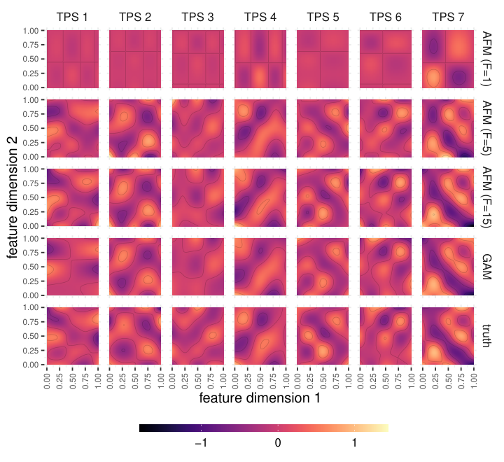
We first compare the estimation performance of our proposal with the SotA for fitting GAMs with TPS. More specifically, we simulate features and generate bivariate non-linear effects for every possible feature pair. The response is generated by adding random noise with a signal-to-noise ratio (SNR) of 0.5 to the sum of all bivariate effects. We then compare the estimation performance of all feature effects qualitatively by inspecting the estimated non-linear effects visually (cf. Figure 2 for ), and quantitatively by computing the mean squared error (MSE) between the estimated and true surfaces (Figure 3). For and (resulting in 10 bivariate effects), we run AFMs with . We repeat every setting 10 times with different random seeds. The GAM estimation can be thought of as a gold standard which is only subject to an estimation error, but no approximation error. In contrast, AFMs are also subject to an approximation error. Our quantitative analysis of results confirms this hypothesis. Figure 3 depicts the MSE differences for all analyzed settings to compare the estimation performance of AFMs and GAMs when calculating the average point-wise differences between the estimated bivariate surface and the true surface. Results suggest that for increasing our approach will approach the estimation performance of GAMs. With more data (larger ), this effect becomes even more
5.2. Prediction Performance
To investigate the prediction performance, we follow the setup from the previous section and compare the prediction performance of the exact GAM and our approach to quantify the approximation error made by the factorization. Figure 4 depicts the results, confirming that the approximation error will tend to zero when increasing the number of observations or latent factors .
5.3. Scalability
Our next experiment investigates the scaling behavior of our approach and compares it to the SotA implementation for big additive models (Wood et al. 2017, BAMs). We simulate standard normal distributed features for observations and fit both BAM and an AFM to learn a GAM with TP splines for all possible combinations of the features. Figure 1 (first page) summarizes the results by comparing the memory consumption (in megabytes) and the computing time (in seconds). The results reflect our initial motivation to propose AFMs. While both time and memory consumption grows exponentially in the number of features for BAMs, we observe a linear scaling for AFMs both for memory consumption and computation time.
5.4. Ablation Benchmark Study
| GLMBoost | GAM | GAMBoost | FM | HOFM() | AFM | AHOFM() | |
|---|---|---|---|---|---|---|---|
| Airfoil | 5.673 (0.290) | 119.3 (2.490) | 4.863 (0.238) | 90.70 (45.55) | 79.03 (51.29) | 4.314 (0.576) | 4.181 (0.699) |
| Concrete | 10.50 (0.969) | 9.768 (8.408) | 6.280 (0.486) | 10.55 (0.970) | 10.56 (0.955) | 6.100 (0.648) | 6.127 (0.491) |
| Diabetes | 55.46 (4.666) | 142.1 (9.626) | 55.18 (5.020) | 143.7 (10.04) | 143.3 (9.312) | 57.12 (6.243) | 63.65 (9.672) |
| Energy | 7.359 (0.631) | 3.409 (0.363) | 3.780 (0.427) | 7.487 (0.620) | 7.480 (0.632) | 3.137 (0.332) | 3.183 (0.359) |
| ForestF | 1.392 (0.098) | 1.465 (0.163) | 1.388 (0.113) | 1.403 (0.105) | 1.398 (0.107) | 1.573 (0.325) | 1.773 (0.307) |
| Naval | 0.013 (0.000) | 0.002 (0.000) | 0.012 (0.000) | 0.009 (0.001) | 0.009 (0.001) | 0.004 (0.002) | 0.003 (0.001) |
| Yacht | 8.991 (1.092) | 3.027 (0.517) | 1.532 (0.546) | 8.883 (0.990) | 8.898 (0.985) | 2.401 (0.618) | 1.743 (0.624) |
To assess the prediction performance of AFMs and AHOFMs on real-world data and better understand their advantages but also their limitations, we compare both approaches against a variety of alternatives with similar properties. In particular, all methods use linear or spline feature effects (i.e., we do not compare against non-additive or tree-based methods), and instead of presenting a benchmark where the proposed methods excel for all data sets, we present various scenarios that allow us to objectively reason about the methods’ pros and cons. More specifically, we compare our methods against GAMs with only univariate smooth terms, FMs, HOFMs, as well as boosting with linear effects (GAMBoost) and boosting with splines (Hothorn et al. 2010, GAMBoost;). Whereas GAMs and GLM-/GAMBoost are tuning-free methods, all factorization approaches are analyzed for only three different numbers of latent dimensions () to provide a more fair comparison. We compare all methods on commonly used benchmark data sets using 10 train-test splits and report average MSE values as well as their standard deviation. Table 1 summarizes the results when choosing the best-performing hyperparameter set per method and data set. Further details on hyperparameters and benchmark data sets can be found in Section E.2 in the Appendix. From our results, the following research hypotheses can be derived: Prediction performance can often be improved by including
- •
interactions (GAMs vs. A(HO)FMs);
- •
non-linearity ((HO)FMs vs. A(HO)FMs);
- •
higher-order interactions (AFM vs. A(HO)FMs).
We can also identify weaknesses of A(HO)FMs. Feature selection (provided by GLM-/GAMBoost but not A(HO)FMs) and inhomogeneous smoothing (GAMBoost) can improve prediction performance. These two aspects are thus a promising direction for future research.
6. Summary and Outlook
We presented an additive model extension of HOFMs to allow for scalable higher-order smooth function estimation based on tensor product splines. The proposed approach allows fitting GAMs with -variate smooth terms at costs similar to a univariate GAM. Our simulation studies showed that when choosing enough latent factors, these machines approximate TPS surfaces very well and match the (almost) exact GAM with TPS both in terms of estimation and prediction performance. A(HO)FMs thereby not only allow to fit higher-order GAMs, but also make additive models more competitive in their predictive performance. This was shown in our benchmark study on real-world data, where the true data-generating process is not necessarily a GAM. Here, AHOFMs improved over the GAM and (HO)FM prediction performance due to the inclusion of interactions and extension to non-linearity. A promising future research direction is the sparsification of the proposed approach. This is also closely related to the interpretability of A(HO)FMs, which we discuss in Appendix D in more detail.
Appendix A Proofs
A.1. Proof of Corollary 4.1
| (18) |
A.2. Proof of Proposition 4.2 and 4.3
Both propositions directly follow from the fact that (18) only sums over , and once, and every basis function is therefore also only evaluated once.
A.3. Proof of Lemma 4.6
An alternative representation of (4.6) is given by
| (19) |
by just plugging in the definition for . We can consider (19) as an ANOVA kernel of degree in the new feature space given by all s. As a result, the multi-linearity property of the ANOVA kernel holds (see Blondel et al. 2016, Appendix B.1), i.e.,
| (20) |
where and therefore AHOFMs can be represented as in Lemma 4.6 by using the same arguments as for HOFMs (Blondel et al. 2016).
A.4. Proof of Lemma B.1
For simplicity assume that the model predictor only consists of a single AHOT, i.e., . The generalization of the following statement to several AHOTs follows due to the additivity of the model predictor. Using Equation 20 and constants , it follows
| (21) |
where , and . (21) shows that is an affine function in . Now let be a convex loss function of and note that in Definition 4.9 is decomposable across the parameters . The composition of and is convex and as is decomposable in and hence also in , the penalized objective in (16) is convex w.r.t. every and thus every .
Appendix B Optimization
Having defined the objective in (16), we obtain the following result.
Lemma B.1.
The optimization problem in (16) is coordinate-wise convex in .
A corresponding proof is given in Appendix A. Using this finding suggests a block coordinate descent (BCD) solver as an alternative approach to optimize (penalized) AHOFMs with block updates for . In contrast to (HO)FMs, we perform block updates instead of plain coordinate descent as the AHOFM penalty is only decomposable w.r.t. all , but not w.r.t. . For BCD we require several quantities:
| (22) |
Note that the first term is involved in every update step, but independent of and the iteration. It is therefore possible to cache the result once at the beginning of the training routine as also mentioned in Algorithm 5. For reverse-mode differentiation, note that the second term can be calculated efficiently by caching intermediate results.
A high-level routine is described in Algorithm 1 (for simplicity for the case with only a single -variate smooth). In Algorithm 1, we require gradients
where is the objective function from (16) and a learning rate , which is defined above. Various terms involved in the update step can be pre-computed or cached (see Appendix C for details).
Appendix C Algorithmic Details
C.1. Demmler-Reinsch Orthogonalization
We here describe the DRO (Algorithm 2) and sv2la (Algorithm 3) routine proposed to efficiently compute smoothing penalties. Details can be found in (Ruppert et al. 2003), Appendix B.1.1. We use Chol to denote the Cholesky decomposition of a matrix and SVD for the singular value decomposition of a matrix.
- (1)
- (2)
C.2. Homogeneous AHOFM Smoothing
Given the previous algorithms, we can implement homogeneous AHOFM smoothing as described in Algorithm 4.
C.3. AHOFM Initialization
Putting everything together, the initialization of AHOFMs is given in Algorithm 5.
- •
using Algorithm 4;
- •
as in (22);
Appendix D Interpretability of A(HO)FMs
Due to their additivity assumption, every additive feature effect in GAMs can be interpreted on its own (ceteris paribus). Although AHOFMs inherit some of the interpretability properties from GAMs, e.g., their additivity, interpreting higher-order (non-linear) interaction terms remains challenging and cannot be done without considering lower-order effects of the same feature. For larger values of , the quickly growing number of additive terms further makes it infeasible to grasp the influence of certain features or interactions. While this is a limitation of the current approach, we here propose three ways to check effects for models with small to moderate . The first approach examines interaction terms by visualizing the single univariate smooth terms for and all involved feature dimensions . Analyzing the univariate latent dimensions separately is not a new approach and the use of factorization approaches can even be motivated by the need to interpret higher-dimensional interactions in lower dimensions (Stöcker and Greven 2021, see, e.g.,). Another approach that focuses only on the interaction effects itself is to visualize the actual approximations as defined in (8). This reduces the number of terms to analyze by the factor , but requires a method for presenting the -variate effect. As shown in Figure 5, a third approach is to visualize the marginals of these multivariate functions together with their variation across the respective other dimensions.
Experiments
We simulate a toy example for with four features to demonstrate the third approach. For better understanding, the features are referred to as time, lat, lon and rate. The outcome is assumed to be normally distributed with and the mean given by the sum of all possible smooth 3-way interactions of the features. To simulate non-linear three-dimensional functions, we use a basis evaluation of features with 4 degrees-of-freedom for time, 5 degrees-of-freedom for lat, 7 degrees-of-freedom for lon and 5 degrees-of-freedom for rate. Partial effects for each three-dimensional smooth are generated by calculating the TP for these basis and randomly drawing coefficients for the resulting TPS. We generate observations, fit a AHOFM() and visualize the resulting effects in two different ways.
Figure 5 depicts the marginal univariate effects of all four features for all four 3-way interaction effects. This allows us to see how each feature marginally affects each of the interaction terms. Additionally, it shows how much variation the marginal effects have in the respective other two dimensions and thereby provides information on how much the features interact with the respective two other variables.
Appendix E Numerical Experiments Details
E.1. Implementation
All methods have been implemented in TensorFlow (Abadi et al. 2016) except for GAMBoost, where we used the package mboost (Hothorn et al. 2010) and the SotA GAM, implemented in mgcv (Wood 2017).
E.2. Benchmark Details
As described in Section 5.4, neither GAMs, (HO)FMs nor AHOFMs have many hyperparameters to tune. We investigate the influence of the latent dimension by testing for all approaches and, for a fair comparison between GAMs and A(HO)FMs, set the values for all methods to the same value . All methods use early stopping on 10% validation data with a patience of 50.
Table 2 further lists the data characteristics for our benchmark data. Pre-processing is only done for ForestF, using a logp1 transformation for area and a numerical representation for month and day.
| Dataset | # Obs. | # Feat. | Reference |
|---|---|---|---|
| Airfoil | 1503 | 5 | (Dua and Graff 2017) |
| Concrete | 1030 | 8 | (Yeh 1998) |
| Diabetes | 442 | 10 | (Efron et al. 2004) |
| Energy | 768 | 8 | (Tsanas and Xifara 2012) |
| ForestF | 517 | 12 | (Cortez and Morais 2007) |
| Naval | 11934 | 16 | (Coraddu et al. 2014) |
| Yacht | 308 | 6 | (Ortigosa et al. 2007; Dua and Graff 2017) |
References
- (1)
- Abadi et al. (2016) Martín Abadi, Paul Barham, Jianmin Chen, Zhifeng Chen, Andy Davis, Jeffrey Dean, Matthieu Devin, Sanjay Ghemawat, Geoffrey Irving, Michael Isard, et al. 2016. Tensorflow: A system for large-scale machine learning. In 12th USENIX symposium on operating systems design and implementation (OSDI 16). 265–283.
- Adomavicius and Tuzhilin (2005) Gediminas Adomavicius and Alexander Tuzhilin. 2005. Toward the next generation of recommender systems: A survey of the state-of-the-art and possible extensions. IEEE transactions on knowledge and data engineering 17, 6 (2005), 734–749.
- Baumann et al. (2021) Philipp Baumann, Torsten Hothorn, and David Rügamer. 2021. Deep Conditional Transformation Models. In Machine Learning and Knowledge Discovery in Databases (ECML-PKDD). Springer International Publishing, 3–18.
- Blondel et al. (2015) Mathieu Blondel, Akinori Fujino, and Naonori Ueda. 2015. Convex factorization machines. In Joint European Conference on Machine Learning and Knowledge Discovery in Databases. Springer, 19–35.
- Blondel et al. (2016) Mathieu Blondel, Akinori Fujino, Naonori Ueda, and Masakazu Ishihata. 2016. Higher-order factorization machines. In Advances in Neural Information Processing Systems. 3351–3359.
- Buja et al. (1989) Andreas Buja, Trevor Hastie, and Robert Tibshirani. 1989. Linear Smoothers and Additive Models. The Annals of Statistics 17, 2 (1989), 453 – 510.
- Chang et al. (2021) Chun-Hao Chang, Rich Caruana, and Anna Goldenberg. 2021. NODE-GAM: Neural Generalized Additive Model for Interpretable Deep Learning. arXiv:2106.01613 [cs.LG]
- Chen et al. (2017) Hong Chen, Xiaoqian Wang, Cheng Deng, and Heng Huang. 2017. Group sparse additive machine. In Proceedings of the 31st International Conference on Neural Information Processing Systems. 197–207.
- Chen et al. (2019) Yifan Chen, Pengjie Ren, Yang Wang, and Maarten de Rijke. 2019. Bayesian Personalized Feature Interaction Selection for Factorization Machines (SIGIR’19). Association for Computing Machinery, New York, NY, USA, 665–674.
- Coraddu et al. (2014) Andrea Coraddu, Luca Oneto, Alessandro Ghio, Stefano Savio, Davide Anguita, and Massimo Figari. 2014. Machine Learning Approaches for Improving Condition-Based Maintenance of Naval Propulsion Plants. Journal of Engineering for the Maritime Environment (2014).
- Cortez and Morais (2007) Paulo Cortez and Aníbal de Jesus Raimundo Morais. 2007. A data mining approach to predict forest fires using meteorological data. (2007).
- Dua and Graff (2017) Dheeru Dua and Casey Graff. 2017. UCI Machine Learning Repository. http://archive.ics.uci.edu/ml
- Efron et al. (2004) Bradley Efron, Trevor Hastie, Iain Johnstone, and Robert Tibshirani. 2004. Least angle regression. The Annals of statistics 32, 2 (2004), 407–499.
- Friedman (2001) Jerome H Friedman. 2001. Greedy function approximation: a gradient boosting machine. Annals of statistics (2001), 1189–1232.
- Hastie and Tibshirani (2017) Trevor J Hastie and Robert J Tibshirani. 2017. Generalized additive models. Routledge.
- Hong et al. (2019) Fuxing Hong, Dongbo Huang, and Ge Chen. 2019. Interaction-aware factorization machines for recommender systems. In Proceedings of the AAAI Conference on Artificial Intelligence, Vol. 33. 3804–3811.
- Hothorn et al. (2010) Torsten Hothorn, Peter Bühlmann, Thomas Kneib, Matthias Schmid, and Benjamin Hofner. 2010. Model-based Boosting 2.0. Journal of Machine Learning Research 11, 71 (2010), 2109–2113.
- Jin et al. (2021) Ruoming Jin, Dong Li, Jing Gao, Zhi Liu, Li Chen, and Yang Zhou. 2021. Towards a Better Understanding of Linear Models for Recommendation. In Proceedings of the 27th ACM SIGKDD Conference on Knowledge Discovery & Data Mining (Virtual Event, Singapore) (KDD ’21). Association for Computing Machinery, New York, NY, USA, 776–785.
- Kingma and Ba (2014) Diederik P Kingma and Jimmy Ba. 2014. Adam: A method for stochastic optimization. arXiv preprint arXiv:1412.6980 (2014).
- Kopper et al. (2021) Philipp Kopper, Sebastian Pölsterl, Christian Wachinger, Bernd Bischl, Andreas Bender, and David Rügamer. 2021. Semi-Structured Deep Piecewise Exponential Models. In Proceedings of AAAI Spring Symposium on Survival Prediction – Algorithms, Challenges, and Applications, PMLR. 40–53.
- Koren et al. (2009) Yehuda Koren, Robert Bell, and Chris Volinsky. 2009. Matrix factorization techniques for recommender systems. Computer 42, 8 (2009), 30–37.
- Lan and Geng (2019) Liang Lan and Yu Geng. 2019. Accurate and Interpretable Factorization Machines. In Proceedings of the AAAI Conference on Artificial Intelligence, Vol. 33. 4139–4146.
- Liu et al. (2008) Han Liu, Larry Wasserman, John Lafferty, and Pradeep Ravikumar. 2008. SpAM: Sparse Additive Models. In Advances in Neural Information Processing Systems, J. Platt, D. Koller, Y. Singer, and S. Roweis (Eds.), Vol. 20. Curran Associates, Inc.
- Lou et al. (2013) Yin Lou, Rich Caruana, Johannes Gehrke, and Giles Hooker. 2013. Accurate intelligible models with pairwise interactions. In Proceedings of the 19th ACM SIGKDD international conference on Knowledge discovery and data mining. 623–631.
- Nelder and Wedderburn (1972) John Ashworth Nelder and Robert WM Wedderburn. 1972. Generalized linear models. Journal of the Royal Statistical Society: Series A (General) 135, 3 (1972), 370–384.
- Nori et al. (2019) Harsha Nori, Samuel Jenkins, Paul Koch, and Rich Caruana. 2019. InterpretML: A Unified Framework for Machine Learning Interpretability. arXiv preprint arXiv:1909.09223 (2019).
- Ortigosa et al. (2007) I Ortigosa, R Lopez, and J Garcia. 2007. A neural networks approach to residuary resistance of sailing yachts prediction. In Proceedings of the international conference on marine engineering MARINE, Vol. 2007. 250.
- Pan et al. (2020) Deng Pan, Xiangrui Li, Xin Li, and Dongxiao Zhu. 2020. Explainable Recommendation via Interpretable Feature Mapping and Evaluation of Explainability. In Proceedings of the Twenty-Ninth International Joint Conference on Artificial Intelligence, IJCAI-20, Christian Bessiere (Ed.). International Joint Conferences on Artificial Intelligence Organization, 2690–2696.
- Rendle (2010) Steffen Rendle. 2010. Factorization machines. In 2010 IEEE International conference on data mining. IEEE, 995–1000.
- Rendle et al. (2020) Steffen Rendle, Walid Krichene, Li Zhang, and John Anderson. 2020. Neural collaborative filtering vs. matrix factorization revisited. In Fourteenth ACM Conference on Recommender Systems. 240–248.
- Rügamer et al. (2023) David Rügamer, Chris Kolb, and Nadja Klein. 2023. Semi-Structured Deep Distributional Regression: A Combination of Additive Models and Deep Learning. The American Statistician (2023).
- Ruppert et al. (2003) D. Ruppert, M.P. Wand, and R.J. Carroll. 2003. Semiparametric Regression. Cambridge University Press.
- Shan and Banerjee (2010) H. Shan and A. Banerjee. 2010. Generalized Probabilistic Matrix Factorizations for Collaborative Filtering. In 2010 IEEE International Conference on Data Mining. 1025–1030.
- Srebro et al. (2004) Nathan Srebro, Jason DM Rennie, and Tommi S Jaakkola. 2004. Maximum-Margin Matrix Factorization.. In NIPS, Vol. 17. Citeseer, 1329–1336.
- Stöcker and Greven (2021) Almond Stöcker and Sonja Greven. 2021. Functional additive regression on shape and form manifolds of planar curves. arXiv preprint arXiv:2109.02624 (2021).
- Tsanas and Xifara (2012) Athanasios Tsanas and Angeliki Xifara. 2012. Accurate quantitative estimation of energy performance of residential buildings using statistical machine learning tools. Energy and Buildings 49 (2012), 560–567.
- Wang et al. (2020) Yingjie Wang, Hong Chen, Feng Zheng, Chen Xu, Tieliang Gong, and Yanhong Chen. 2020. Multi-task Additive Models for Robust Estimation and Automatic Structure Discovery. In Advances in Neural Information Processing Systems, H. Larochelle, M. Ranzato, R. Hadsell, M. F. Balcan, and H. Lin (Eds.), Vol. 33. Curran Associates, Inc., 11744–11755.
- Wood (2006) Simon N. Wood. 2006. Low-Rank Scale-Invariant Tensor Product Smooths for Generalized Additive Mixed Models. Biometrics 62, 4 (2006), 1025–1036.
- Wood (2017) Simon N Wood. 2017. Generalized additive models: an introduction with R. Chapman and Hall/CRC.
- Wood et al. (2017) Simon N. Wood, Zheyuan Li, Gavin Shaddick, and Nicole H. Augustin. 2017. Generalized Additive Models for Gigadata: Modeling the U.K. Black Smoke Network Daily Data. J. Amer. Statist. Assoc. 112, 519 (2017), 1199–1210.
- Yeh (1998) I-C Yeh. 1998. Modeling of strength of high-performance concrete using artificial neural networks. Cement and Concrete research 28, 12 (1998), 1797–1808.
- Yin et al. (2012) Junming Yin, Xi Chen, and Eric P Xing. 2012. Group sparse additive models. In Proceedings of the… International Conference on Machine Learning. International Conference on Machine Learning, Vol. 2012. NIH Public Access, 871.
- Yuan et al. (2017) Fajie Yuan, Guibing Guo, Joemon M. Jose, Long Chen, Haitao Yu, and Weinan Zhang. 2017. BoostFM: Boosted Factorization Machines for Top-N Feature-Based Recommendation. In Proceedings of the 22nd International Conference on Intelligent User Interfaces (IUI ’17). Association for Computing Machinery, New York, NY, USA, 45–54.
- Zhang et al. (2016) XianXing Zhang, Yitong Zhou, Yiming Ma, Bee-Chung Chen, Liang Zhang, and Deepak Agarwal. 2016. GLMix: Generalized Linear Mixed Models For Large-Scale Response Prediction (KDD ’16). Association for Computing Machinery, New York, NY, USA, 363–372.
- Zhuang et al. (2021) Honglei Zhuang, Xuanhui Wang, Michael Bendersky, Alexander Grushetsky, Yonghui Wu, Petr Mitrichev, Ethan Sterling, Nathan Bell, Walker Ravina, and Hai Qian. 2021. Interpretable Ranking with Generalized Additive Models. In Proceedings of the 14th ACM International Conference on Web Search and Data Mining (Virtual Event, Israel) (WSDM ’21). Association for Computing Machinery, New York, NY, USA, 499–507.