A Multicritical Point with Infinite Fractal Symmetries
Abstract
Recently a “Pascal’s triangle model” constructed with rotor degrees of freedom was introduced, and it was shown that (i.) this model possesses an infinite series of fractal symmetries; and (ii.) it is the parent model of a series of fractal models each with its own distinct fractal symmetry. In this work we discuss a multi-critical point of the Pascal’s triangle model that is analogous to the Rokhsar-Kivelson (RK) point of the better known quantum dimer model. We demonstrate that the expectation value of the characteristic operator of each fractal symmetry at this multi-critical point decays as a power-law of space, and this multi-critical point is shared by the family of descendent fractal models. Afterwards, we generalize our discussion to a model termed the “Pascal’s tetrahedron model” that has both planar and fractal subsystem symmetries. We also establish a connection between the Pascal’s tetrahedron model and the Haah’s code.
I Introduction
In recent years we have seen a very fruitful exploration of generalizing the concept of “symmetry” in physics. It was demonstrated that introducing the concept of higher form symmetries is very useful for studying gauge fields Nussinov and Ortiz 2009; Aharony et al. 2013; Gukov and Kapustin 2013; Kapustin and Thorngren 2013a; Kapustin and Thorngren 2013b; Kapustin and Seiberg 2014; Gaiotto et al. 2015; Hsin et al. 2019; Seiberg 2020; McGreevy 2022; in particular the analysis of the ’t Hooft anomaly of higher form symmetries can lead to very clear and nontrivial conclusion for the low energy physics of gauge fields with a topological term Gaiotto et al. 2017. Another set of generalized symmetries have their conserved charges defined on a subset of the system Nandkishore and Hermele 2019; Pretko et al. 2020, and these “subsystem symmetries” can be further categorized into type-I, when the symmetric charges are defined on regular subsystems such as lines and planes, and type-II, when the symmetric charges reside on a fractal subsystem with often non-integer Hausdorff dimensions. So far systems with type-I subsystem symmetries are better understood, as not only can one study the lattice models with type-I subsystem symmetries, for gapless states (or phases) with type-I subsystem symmetry, it is also possible to describe the states with low energy effective theories which are constructed only with the low energy subspace of the Hilbert space rather than all the microscopic degrees of freedom of the system. One classic example of such was constructed by Paramekanti, Balents, Fisher in Ref. Paramekanti et al. 2002 (dubbed the XY-plaquette model). The authors constructed a quantum rotor model with one dimensional conservation of rotor numbers, and the authors studied in great detail a gapless state of this model. A low energy effective theory constructed with low energy modes of the system was developed for this gapless state, and a lot of physics can be studied systematically with the low energy effective theory. It was demonstrated that standard methods such as renormalization group (RG) can still be applied to the gapless state of the XY-plaquette model despite its highly unusual symmetries. The XY-plaquette model along with its low energy effective theory was later generalized to various models in higher dimensions, and it has attracted much enthusiasm recently Xu and Fisher 2007; Ma and Pretko 2018; You et al. 2020; Yuan et al. 2020; Gromov et al. 2020; Seiberg and Shao 2021; Rudelius et al. 2021; Gorantla et al. 2021; Burnell et al. 2021.
By the same standard, systems with type-II subsystem symmetries (or fractal symmetries), are much less understood. Much success was accomplished through studying exactly soluble lattice models such as the Haah’s code Haah 2011, but a low energy effective theory which does not involve all the microscopic degrees of freedom is more challenging compared with systems with type-I subsystem symmetries. Of course, a low energy effective theory may not be necessary if one only studies gapped states of type-II models, as under renormalization group (RG) flow gapped states are expected to “flow to” an exactly soluble lattice model as the fixed point of the entire gapped phase, although a proper procedure of RG has not been developed for systems with fractal symmetries. But recent numerics suggests that a continuous quantum phase transition may exist for models with fractal symmetries Zhou et al. 2021 (we note that earlier numerics suggested the opposite Vasiloiu et al. 2020), this calls for an understanding of gapless states with fractal symmetries at the same level as regular systems. A low energy effective theory will go a long way towards understanding the universal physics of such gapless systems without relying too much on the lattice models.
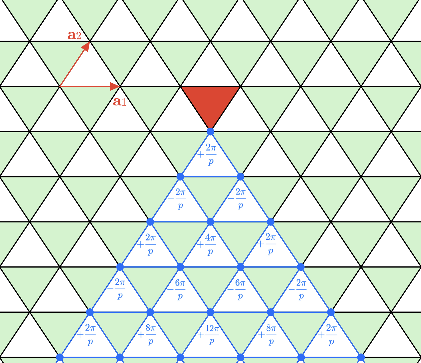
In this work we construct a gapless state with an infinite series of fractal symmetries. The model we will start with was called the “Pascal’s triangle model”:
| (1) |
where the boson phase and boson number are a pair of conjugate variables which obey the usual algebra . This Hamiltonian exhibits a conventional global symmetry involving rotating on any two of the three sublattices of the triangular lattice by an opposite angle. This model was introduced for the purpose of understanding the quantum phase transition of the Sierpinski triangle model Zhou et al. 2021, but it was pointed out in Ref. Myerson-Jain et al. 2022 that this model actually supports a much larger group of fractal symmetries. In fact, the model possesses an infinite collection of distinct fractal symmetries (one for each prime integer ) which together are called the “Pascal’s triangle symmetry” that involve a staggered rotation of the boson phase with support on a Pascal’s triangle mod . The action of this symmetry on a local patch of the lattice is generated by the so-called “patch symmetry operator” of the Pascal’s triangle symmetry
| (2) | |||||
| (4) |
The sum in the patch charge is over a triangular region of length (centered at the origin, . The action of the patch symmetry operator is shown in Fig. 1. It was demonstrated in Ref. Myerson-Jain et al. 2022 that for system sizes of , the fractal symmetry becomes exact. The Pascal’s triangle model also reduces to a family of descendent -clock model Hamiltonians that exhibit only a single one of its fractal symmetries. For example if one reduces the rotor degree of freedom to an Ising spin, the Pascal’s triangle model reduces to the Sierpinski triangle model Newman and Moore 1999; Yoshida 2013.
II Multi-critical point of the Pascal’s triangle model
II.1 Dual of the Pascal’s triangle model
The dual variables were introduced to understand the physics of the Pascal’s triangle model Myerson-Jain et al. 2022 Eq. 1:
| (5) |
where label the sites of the original and dual lattices respectively. is a discrete variable and is its conjugate compact variable that satisfies the bosonic algebra . The Hamiltonian Eq. 1 is now dual to a height model:
| (6) |
We analyze this dual height model following the standard procedure. We first expand the height model to the quadratic order and add a vertex operator that re-enforces the compactness of (or discreteness of ), then can be treated as a continuous variable:
| (7) |
A Euclidean action describing this model can be attained by expanding the Gaussian part of about the minima of the spectrum which occur at the points in the Brillouin zone (BZ). After expanding the height operator
| (8) |
and taking the continuum limit, the low energy physics of the height model is supposedly described by the Lagrangian
| (9) |
To avoid potential confusion, we clarify that throughout this paper, the phrase continuum limit simply means the limit where the system size is taken to infinity while keeping a constant lattice spacing. Eq. 9 becomes an effective description of the lattice model when the field is a smooth function on the lattice. The two component vector field is and label the three sublattices of the dual triangular lattice with , , . Analogous to the analysis of instantons in compact , due to the linear dispersion modes of the height field, the coefficient of the vertex operators is strongly relevant. As a consequence, we conclude that the gapless modes of the Gaussian theory of the height model are unstable; or in other words the generic Pascal’s triangle model should in general be in a gapped quantum disordered phase, just like the compact QED3 should be in a confined phase without fine-tuning. The connection between the Pascal’s triangle model and QED3 will be made more explicit later.
II.2 Multi-critical point
Although the vertex operators (the -terms) in Eq. 9 destroy the gapless modes of the Gaussian theory of the dual height model, they can be suppressed to restore the gaplessness of the spectrum by fine-tuning the model to a multi-critical point. This multi-critical point has a simple description in terms of the dual height field:
| (10) |
This Lagrangian is two copies of the quantum Lifshitz theory, which is pertinent to the study of the RK point of the quantum dimer model in Rokhsar and Kivelson 1988; FRADKIN and KIVELSON 1990; Fradkin et al. 2004; Ardonne et al. 2004; Vishwanath et al. 2004. This theory is the analogue of the massless boson CFT in and is known to be stable against vertex operators for some range of . In particular, the -function for the vertex operators to the leading order is
| (11) |
Later we will further demonstrate that this multi-critical point is shared by all the descendent fractal models of the Pascal’s triangle model. We can conclude that the vertex operators are irrelevant when Fradkin et al. 2004.
Returning to lattice model Eq. 1, the multi-critical point can be reached by turning on nearest neighbor density-density interactions
| (12) | |||
| (13) | |||
| (14) |
which changes the band structure of the dual height model. A band structure calculation shows that by fine-tuning to certain point, the dispersion of the height field becomes quadratic.
However, we must be careful since there are possible relevant operators and other marginal operators that may appear in RG that must be tuned to zero. These operators must obey the point-group symmetries of the lattice Hamiltonian. The scaling dimensions of space-time coordinates, and operators in the Lifshitz theory are , and . An example of a relevant operator that must be tuned to zero is
| (15) |
This operator is similar to the one discussed in the context of quantum dimer model on the honeycomb lattice Fradkin et al. 2004. Several other operators such as are marginal at the Lifshitz theory by power-counting, but they may become marginally relevant after considering quantum fluctuations Vishwanath et al. 2004. These perturbations had better also be tuned to zero to ensure the system stays at the multi-critical point.
II.3 Characteristic features at the multi-critical point
To probe the physics at the multi-critical point, we would like to compute the expectation value of some characteristic operators. In particular we need an operator whose expectation value can distinguish different phases of a quantum many-body system. For a system with a symmetry, the so called “patch operator” defined as symmetry transformation operation localized on a patch can serve as a diagnosis of the phase Ji and Wen 2020. This operator was also referred to as the “disorder operator” for the example of Ising model in previous literature Kadanoff and Ceva 1971, and later generalized to systems with type-I subsystem symmetries Wu et al. 2021a as the order diagnosis operator. The application of the patch operator can be exemplified in the quantum Ising model: the patch operator has short range, power-law, and long range expectation value in the Ising ordered phase, critical point, and the Ising disordered phase respectively (the exact opposite from the correlation function of the Ising order parameter). For more general cases, the expectation value of the patch operator should have a qualitative enhancement in a quantum disordered phase compared with the critical point. In the last few years the patch operators have been evaluated for various systems, it was shown that useful information can be extracted from the expectation value of the patch operator Zhao et al. 2021; Wu et al. 2021b; Wang et al. 2021a; Wang et al. 2021b.
Here we compute the expectation value of the patch operator of the Pascal’s triangle symmetry Eq. 4. As explained, opposed to the more standard order parameter, a long-range expectation value signifies a disordered phase. Power-law decay, however, still identifies a critical point. In terms of the dual variables of the height model, the Pascal’s triangle symmetry charge on a patch of length with the left corner at the origin becomes
| (16) |
where the support of the charge on a patch completely cancels in the bulk of the patch in the dual variables, and the remaining support is on the top corner and bottom row of the triangular region. However, since is always an integer multiple of for , the patch symmetry operator simplifies even further to involve only three operators at the corners of the patch:
| (17) |
Let us use lattice vectors of the triangular lattice and where and are the usual Cartesian unit vectors. is at the top corner of the triangle in the dual representation, while and are located at the bottom left and right corners of the Pascal’s triangle respectively. For simplicity, we first consider the case where when . We will return to the case of and later. After expanding around the points we have that
For , and . So we have after expanding . Since and are uncoupled in the Lagrangian, the expectation of factorizes into the product of two simpler correlators
| (18) | |||||
| (20) | |||||
| (22) |
Here the Euclidean propagator is computed according to a single copy of the Lifshitz theory. It is known that the propagator is logarithmic,
| (23) |
is the momentum cutoff. Since the propagator only depends on the distance , and our fields lie at the corners of an equilateral of length , becomes
| (24) |
Hence, the patch symmetry operator decays as a power-law with exponent .
For , the calculation is exactly the same but we must be careful since now. However, since the original height fields are quantized, as the operator , the latter operator having a sensible algebriac decay computable in the Lifshitz theory with exponent .
Now for , all lie on the same sublattice. As a consequence, after expansion we have
Again making use of the fact that the initial fields were quantized we can compute the correlation of . The latter form of the operator is an observable which has sensible decay once computed in the Lifshitz theory. This is because the sum of coefficients in front of the fields vanishes in this form, a necessary requirement to find a non-trivial result for the correlation function. After expansion, we must compute in the Lifshitz theories
| (25) | |||||
| (27) | |||||
| (29) |
This is a slightly stronger decay than we found for , though the decay remains power-law. Hence, we conclude that the decay of the patch symmetry operator at the multi-critical point is with this exponent being twice as large for .
We can compare the behavior of the patch operator at the multi-critical point versus in the disordered phase, which as we argued before is the generic phase of the model Eq. 1. Inside the disordered phase, the vertex operator is relevant, and is pinned at the minima of the vertex operators, with suppressed fluctuation. In this case, decays exponentially with distance, hence is expected to saturate to a finite value with long distance. This is consistent with the intuition one gather from other models: in the disordered phase, the disorder operator usually has enhanced correlation compared with the critical point.
II.4 Multi-criticality of descendent models
We have shown that upon fine-tuning the Pascal’s triangle model, it can reach a multi-critical point. We can consider if there exists a similar multi-critical point for the descendent fractal models with one of the fractal symmetries. For example, a descendent fractal model can be constructed by adding an operator to the theory that energetically favors the eigenvalues of the boson phase to be valued. The appropriately perturbed Pascal’s triangle model is
| (30) |
Where is given by Eq. 1. If the anisotropy is irrelevant at the multi-critical point discussed above, then we can conclude that all fractal models attained by (weakly) breaking the rotor degrees of freedom down share the same multi-critical point as the Pascal’s triangle model upon some fine-tuning.
To analyze the relevance of the anisotropy, we need to evaluate the perturbation of the operator in Eq. 30 at the multi-critical point discussed above. If an operator is relevant, it would make infrared divergent contribution to the partition function at certain order of perturbation. For example, in the XY-plaquette model, If one turns on the same anisotropy , the fourth order perturbation of will have nonzero expectation value at the fixed point with , as long as the four operators are located at the four corners of a rectangle Paramekanti et al. 2002, as required by the type-I subsystem symmetry. Though this expectation value decays with the size of the rectangle, it was shown that it can lead to infrared divergent contribution to the partition function, especially when the operators are paired up as dipoles. Hence the anisotropy can generate relevant dipole operators. But in our case, one can verify that, in order to preserve the fractal symmetries at the multi-critical point, at any finite order of perturbation of , the expectation value always vanishes at large distance due to violation of the Pascal’s triangle symmetry. Another way to look at the difference between our case and the XY-plaquette model is that, the nonzero four point correlation function of the XY-plaquette model can be viewed as the product of the term in the Hamiltonian over a rectangular area; but in our case a product of over certain area does not reduce to a simple finite composite operator when is large.
We stress here that, our argument for being irrelevant is based on perturbative expansion of at the fine-tuned fixed point where takes continuous value. This argument is only supposed to hold for weak anisotropy.
II.5 Relation of the Pascal’s triangle model to a gauge theory
Apart from the duality between the Pascal’s triangle model and the height model, there exists another separate representation of the Pascal’s triangle model in terms of a gauge theory. As we discussed in previous subsections, the dual height model of the Pascal’s triangle model has two components of scalar fields at low energy, then following the standard “boson-vortex” duality procedure Peskin 1978; Dasgupta and Halperin 1981; Fisher and Lee 1989, the dual of the height model should be two gauge fields. In this section we explore the relation between the Pascal’s triangle model and a gauge theory.
We define the canonical conjugate fields and on the sites of a honeycomb lattice as
| (31) | |||
| (32) | |||
| (33) | |||
| (34) | |||
| (35) |
where and are the two sublattices of the honeycomb lattice. This honeycomb lattice has the original triangular lattice as one of its sublattices, say . The electric fields are forced to obey the Gauss’ law constraint
| (36) |
The Hamiltonian of the resultant model, which we will refer to as the “six-boson model”, is
| (37) |

In addition, this six-boson model is directly related to the Pascal’s triangle model with or without fine-tuning by gauge fixing. The gauge symmetry generated by the Gauss operator transforms the gauge fields according to
| (38) |
There is actually a valid gauge where the gauge fields on one of the two sublattices is completely gauged away. A gauge transformation that sets any single to zero and does not change any other is shown in Fig. 2. Using this gauge transformation, an accumulative gauge transformation can be constructed that fixes the gauge field to be zero at every site in the sublattice. This is achieved by making the following choice for every appropriately:
| (39) |
Specifically for where is the honeycomb whose top corner is at the origin, the appropriate region being summed over is .
Despite the form of the gauge transformation in Eq. 38, the gauge group of the six-boson model is actually . This should be expected from duality as each of the two scalar fields of the height model is dual to a gauge field in . As a consequence, there are two sets of Gauss’ law constraints that generate two separate gauge transformations: one set where each lies on two of the sublattices of the dual triangular lattice and a second set where each lies on a different choice of two sublattices. The gauge group can also be directly verified in the continuum limit of the Gaussian approximation of Eq. 37. After the gauge fields are expanded around the points in the BZ, the six-boson model reduces to two copies of QED3 up to a field redefinition.
Other correlation functions of the Pascal’s triangle model at the multi-critical point may be computed using the six-boson model. In particular, Wilson loops of the six-boson model end up reducing to correlation functions of products of the three-body operator in the gauge. These Wilson loops are given by staggered sums of the six-body interactions in some region so that the support in the bulk cancels and what remains is a loop of staggered gauge fields on the boundary. More precisely,
| (40) | |||||
| (42) |
after a relabeling of as .
In addition, the Lifshitz theory is known to have a duality to a gauge theory. In particular, the field theory of the fine-tuned height model at the multi-critical point is dual to
| (43) | |||||
| (45) |
for two gauge fields and . This implies that the low energy theory of a fine-tuned version of the six-boson model, which reduces to the appropriate fine-tuned Pascal’s triangle model, is equal to Eq. 45 up to a redefinition of the gauge fields.

It is known that the Wilson loops decay as a perimeter law in this theory, Eq. 45. As this is the case, correlation functions of products of the three-body term in the Pascal’s triangle model will also decay as a perimeter law. On the triangular lattice, we can consider a local patch let us denote as . This patch contains a set of downward plaquettes which in themselves form the sites of the dual triangular lattice. If we now take a product of the three-body operators on two of the three dual sublattices of the plaquettes inside staggered on one of the sublattices, we recover an operator that is a product of with support only on . That is,
| (46) |
where depending on whether on the boundary lies on a downward triangle on the sublattices of the dual triangular lattice. However, this operator is really just a Wilson loop of the six-boson model in the gauge of the form Eq. 42 and hence decays as a perimeter law with the number of boson phases on . This is explicitly shown in Fig. 3. But in the quantum disordered phase, which is the generic phase of either the Pascal’s triangle model or the six-boson model, the Wilson loop will decay with an area law. In terms of the gauge theory language the quantum disordered phase is the confined phase. The area law can be shown by starting with the ground state with large , and perform perturbation of operator in the Hamiltonian.
III Pascal’s tetrahedron model
III.1 The Hamiltonian and its symmetries
There is a natural generalization of the Pascal’s triangle model to which we refer to as the Pascal’s tetrahedron model. On the cubic lattice, the Hamiltonian of the Pascal’s tetrahedron model reads
| (47) |
The four-body interaction involves the sum of boson phases over a tetrahedron on the cubic lattice; it is the natural generalization of the three-body interaction of Eq. 1. The “Pascal’s tetrahedron symmetries” are also made up of an infinite series of fractal symmetries. The action of the fractal symmetries on a finite tetrahedron with top corner at the origin of length is generated by the following patch symmetry operator
| (48) | |||||
| (50) |
The action of this operator rotates the boson phase according to on the tetrahedral region . Successive transformations of this form over extensively large regions will give rise to exact fractal symmetries, e.g. an exact fractal symmetry with can be generated by three of these transformations for lattice size .
Despite Eq. 47 being the straightforward generalization of the Pascal’s triangle model to , the Pascal’s tetrahedron model manifests another type-I planar subsystem symmetry of which there is no analogue in . We may decompose the cubic lattice into four sublattices each spanned by vectors . The first sublattice is given by and the other three are obtained from subsequent shifts by and respectively. Now, consider a plane on the cubic lattice with normal . We construct this plane by where and is attained from by a shift of . The Pascal’s tetrahedron model is invariant under the following transformation on :
| (51) |
Translations of the support of this transformation in the and directions will be exact symmetries as well. Furthermore, there exist two other sets of mutually orthogonal planes with normals of which a staggered rotation such as Eq. 51 leaves the Pascal’s tetrahedron model invariant. These collection of planar transformations form the entire planar symmetry of Eq. 47.
In the classical limit of the Pascal’s tetrahedron model (), there exist both domain walls and fractonlike excitations. Firstly there exist fractonlike excitations created at the tetrahedra located at the corners of a Pascal’s tetrahedron mod by acting with the fractal transformation in a local patch. Like the case, these excitations cost energy above the configuration. In addition, there are one-dimensional loop excitations analogous to domain walls of the XY model created by acting with the symmetry on a patch of a plane such as . Starting with the uniform configuration , these loop excitations cost an energy of above such a ground-state configuration.
There is a dual of the Pascal’s tetrahedron model similar to that of Eq. 6. If we define variables on the dual cubic lattice whose lattice sites are located at the center of the cubes of the original lattice
| (52) | |||||
| (54) |
Such a mapping preserves the bosonic algebra, and yields a dual height model of the Pascal’s tetrahedron model
| (55) |
This duality involving the , or Sierpinski-tetrahedron, version of this model was pointed out in Ref. Garrahan 2002; Devakul et al. 2019.
This dual height model does not explicitly possess the Pascal’s tetrahedron symmetries of the original model as the fields are discrete, though it does retain a dual version of the symmetry. This dual subsystem symmetry is realized in the spectrum via nodal lines of zero energy modes. It is straightforward to calculate the spectrum of the height model as . Despite the modest form of the Hamiltonian and the spectrum, we know that the height model has a dual symmetry and so its spectrum must display nodal lines where . In fact there are six nodal line segments in the BZ, e.g. . If expanded along this line, the dispersion of the height field becomes
| (56) | |||||
| (58) |
As a consequence, an analysis of a potential multicritical point of the Pascal’s tetrahedron model must involve a similar height field expansion as in the analysis in , but around each of the nodal lines. We leave the detailed discussion of the RK point of tetrahedron model to future studies.


III.2 Relation to the U(1) Haah’s code
Like the Pascal’s triangle model, the Pascal’s tetrahedron model is related to a gauge theory by gauge fixing. However, while in the this theory was a conventional gauge theory, we will show that the appropriate gauge theory in is the pure (i.e. uncoupled from matter, the Gauss’ operator is non-dynamical) version of the Haah’s code. The dual height model in Eq. 55 has a second duality. We can define two new electric and gauge fields according to
| (59) | |||||
| (61) | |||||
| (63) | |||||
| (65) |
The version of this mapping is equivalent to the “F-S” duality outlined in Ref. Vijay et al. 2016. There exists a linear combination of interactions of the form and that vanishes, and as a result the electric fields of the dual must obey the corresponding Gauss’ law constraint this time being
| (66) | |||||
| (68) |
The Hamiltonian of the resulting gauge theory takes the form of the rotor limit of pure Haah’s code
| (69) | |||||
| (71) | |||||
| (73) |
Reducing the degrees of freedom to Ising spins via and , leaves us with a perturbed version of the pure Haah’s code. Fractional gauge fluxes of this model created at the corners of products of or in the shape of Pascal’s tetrahedra mod will be completely immobile fractons. As each of these fractons costs an energy in the classical limit ().
The Gauss operator generates a gauge transformation acting on the gauge fields of
| (74) | |||||
| (76) |
The pure Haah’s code can be reduced to the Pascal’s tetrahedron model upon gauge fixing and tuning of the electric couplings. We may choose
| (77) |
with tetrahedral region being that of with the opposite orientation centered at site . Such a transformation sets at every site as with this choice, yielding exactly the Pascal’s tetrahedron model. This should be expected given the dualities we have just described; our pure Haah’s code is dual to the height model Eq. 55 which in turn is dual to Eq. 47, and hence must be dynamically equivalent to the Pascal’s tetrahedron model.
Since the height field in the dual representation of the tetrahedron model is a scalar field, then one would expect that the dual of a scalar field is a 2-form gauge field in three dimensional space. And a 2-form gauge field should have “Wilson membranes” rather than Wilson lines. Indeed, one can show that gauge invariant operators constructed as staggered products of the -operator, in Eq. 73, in a three dimensional bulk of the system reduces to surface products of and (Fig. 4). Specifically, one can consider a box shaped patch of the cubic lattice. As each cube inside the patch belongs to one of the four sublattices of the dual cubic lattice, a product of -operators staggered on two of the dual sublattices reduces to an operator which only has remaining support on the boundary of the patch. This operator appropriately reduces to a product of boson phases in the boundary of the patch in the Pascal’s tetrahedron model upon gauge fixing.
IV Discussion
In this work we constructed a gapless multi-critical point from a lattice model with an infinite series of fractal symmetries, which together are called the Pascal’s triangle symmetry. This multi-critical point can be reached by tuning a finite number of parameters of the generic Pascal’s triangle model, and it is analogous to the RK point of the quantum dimer model in the sense that it is gapless with a dispersion. At this multi-critical point, physics can be analyzed conveniently in the dual description of the system; and we demonstrate that the characteristic “patch operators” of all the fractal symmetries have an expectation value that decay with a power law of space, which is usually a sign of criticality. Potential generalizations to three dimensional systems are also discussed, but we leave an in-depth discussion of a potential RK point of the Pascal’s tetrahedron model to a future work. As we mentioned earlier, gapless states with type-I subsystem symmetries have been studied quite extensively since Ref. Paramekanti et al. 2002, we hope our work can draw attention to the study of gapless systems with type-II fractal symmetries.
We would like to acknowledge Sagar Vijay and Shang Liu for insightful discussions. This work is supported by NSF Grant No. DMR-1920434, and the Simons Investigator program. Part of the discussions in this work originated from an unpublished work with Ashvin Vishwanath many years back.
References
- Nussinov and Ortiz (2009) Z. Nussinov and G. Ortiz, Annals of Physics 324, 977 (2009), ISSN 0003-4916, URL http://dx.doi.org/10.1016/j.aop.2008.11.002.
- Aharony et al. (2013) O. Aharony, N. Seiberg, and Y. Tachikawa, Journal of High Energy Physics 2013 (2013), ISSN 1029-8479, URL http://dx.doi.org/10.1007/JHEP08(2013)115.
- Gukov and Kapustin (2013) S. Gukov and A. Kapustin (2013), eprint 1307.4793.
- Kapustin and Thorngren (2013a) A. Kapustin and R. Thorngren (2013a), eprint 1308.2926.
- Kapustin and Thorngren (2013b) A. Kapustin and R. Thorngren (2013b), eprint 1309.4721.
- Kapustin and Seiberg (2014) A. Kapustin and N. Seiberg, Journal of High Energy Physics 2014 (2014), ISSN 1029-8479, URL http://dx.doi.org/10.1007/JHEP04(2014)001.
- Gaiotto et al. (2015) D. Gaiotto, A. Kapustin, N. Seiberg, and B. Willett, Journal of High Energy Physics 2015 (2015), ISSN 1029-8479, URL http://dx.doi.org/10.1007/JHEP02(2015)172.
- Hsin et al. (2019) P.-S. Hsin, H. T. Lam, and N. Seiberg, SciPost Physics 6 (2019), ISSN 2542-4653, URL http://dx.doi.org/10.21468/SciPostPhys.6.3.039.
- Seiberg (2020) N. Seiberg, SciPost Physics 8 (2020), ISSN 2542-4653, URL http://dx.doi.org/10.21468/SciPostPhys.8.4.050.
- McGreevy (2022) J. McGreevy, Generalized symmetries in condensed matter (2022), URL https://arxiv.org/abs/2204.03045.
- Gaiotto et al. (2017) D. Gaiotto, A. Kapustin, Z. Komargodski, and N. Seiberg, Journal of High Energy Physics 2017 (2017), URL https://doi.org/10.1007%2Fjhep05%282017%29091.
- Nandkishore and Hermele (2019) R. M. Nandkishore and M. Hermele, Annual Review of Condensed Matter Physics 10, 295 (2019), eprint https://doi.org/10.1146/annurev-conmatphys-031218-013604, URL https://doi.org/10.1146/annurev-conmatphys-031218-013604.
- Pretko et al. (2020) M. Pretko, X. Chen, and Y. You, International Journal of Modern Physics A 35, 2030003 (2020), eprint https://doi.org/10.1142/S0217751X20300033, URL https://doi.org/10.1142/S0217751X20300033.
- Paramekanti et al. (2002) A. Paramekanti, L. Balents, and M. P. A. Fisher, Phys. Rev. B 66, 054526 (2002), URL https://link.aps.org/doi/10.1103/PhysRevB.66.054526.
- Xu and Fisher (2007) C. Xu and M. P. A. Fisher, Phys. Rev. B 75, 104428 (2007), URL https://link.aps.org/doi/10.1103/PhysRevB.75.104428.
- Ma and Pretko (2018) H. Ma and M. Pretko, Phys. Rev. B 98, 125105 (2018), URL https://link.aps.org/doi/10.1103/PhysRevB.98.125105.
- You et al. (2020) Y. You, Z. Bi, and M. Pretko, Phys. Rev. Research 2, 013162 (2020), URL https://link.aps.org/doi/10.1103/PhysRevResearch.2.013162.
- Yuan et al. (2020) J.-K. Yuan, S. A. Chen, and P. Ye, Phys. Rev. Research 2, 023267 (2020), URL https://link.aps.org/doi/10.1103/PhysRevResearch.2.023267.
- Gromov et al. (2020) A. Gromov, A. Lucas, and R. M. Nandkishore, Phys. Rev. Research 2, 033124 (2020), URL https://link.aps.org/doi/10.1103/PhysRevResearch.2.033124.
- Seiberg and Shao (2021) N. Seiberg and S.-H. Shao, SciPost Physics 10 (2021), URL https://doi.org/10.21468%2Fscipostphys.10.2.027.
- Rudelius et al. (2021) T. Rudelius, N. Seiberg, and S.-H. Shao, Phys. Rev. B 103, 195113 (2021), URL https://link.aps.org/doi/10.1103/PhysRevB.103.195113.
- Gorantla et al. (2021) P. Gorantla, H. T. Lam, N. Seiberg, and S.-H. Shao, Phys. Rev. B 104, 235116 (2021), URL https://link.aps.org/doi/10.1103/PhysRevB.104.235116.
- Burnell et al. (2021) F. J. Burnell, T. Devakul, P. Gorantla, H. T. Lam, and S.-H. Shao, Anomaly inflow for subsystem symmetries (2021), URL https://arxiv.org/abs/2110.09529.
- Haah (2011) J. Haah, Phys. Rev. A 83, 042330 (2011), URL https://link.aps.org/doi/10.1103/PhysRevA.83.042330.
- Zhou et al. (2021) Z. Zhou, X.-F. Zhang, F. Pollmann, and Y. You (2021), eprint 2105.05851.
- Vasiloiu et al. (2020) L. M. Vasiloiu, T. H. E. Oakes, F. Carollo, and J. P. Garrahan, Phys. Rev. E 101, 042115 (2020), URL https://link.aps.org/doi/10.1103/PhysRevE.101.042115.
- Myerson-Jain et al. (2022) N. E. Myerson-Jain, S. Liu, W. Ji, C. Xu, and S. Vijay, Phys. Rev. Lett. 128, 115301 (2022), URL https://link.aps.org/doi/10.1103/PhysRevLett.128.115301.
- Newman and Moore (1999) M. E. J. Newman and C. Moore, Phys. Rev. E 60, 5068 (1999), URL https://link.aps.org/doi/10.1103/PhysRevE.60.5068.
- Yoshida (2013) B. Yoshida, Phys. Rev. B 88, 125122 (2013), URL https://link.aps.org/doi/10.1103/PhysRevB.88.125122.
- Rokhsar and Kivelson (1988) D. S. Rokhsar and S. A. Kivelson, Phys. Rev. Lett. 61, 2376 (1988), URL https://link.aps.org/doi/10.1103/PhysRevLett.61.2376.
- FRADKIN and KIVELSON (1990) E. FRADKIN and S. KIVELSON, Modern Physics Letters B 04, 225 (1990), eprint https://doi.org/10.1142/S0217984990000295, URL https://doi.org/10.1142/S0217984990000295.
- Fradkin et al. (2004) E. Fradkin, D. A. Huse, R. Moessner, V. Oganesyan, and S. L. Sondhi, Phys. Rev. B 69, 224415 (2004), URL https://link.aps.org/doi/10.1103/PhysRevB.69.224415.
- Ardonne et al. (2004) E. Ardonne, P. Fendley, and E. Fradkin, Annals of Physics 310, 493 (2004), ISSN 0003-4916, URL https://www.sciencedirect.com/science/article/pii/S0003491604000247.
- Vishwanath et al. (2004) A. Vishwanath, L. Balents, and T. Senthil, Phys. Rev. B 69, 224416 (2004), URL https://link.aps.org/doi/10.1103/PhysRevB.69.224416.
- Ji and Wen (2020) W. Ji and X.-G. Wen, Phys. Rev. Research 2, 033417 (2020), URL https://link.aps.org/doi/10.1103/PhysRevResearch.2.033417.
- Kadanoff and Ceva (1971) L. P. Kadanoff and H. Ceva, Phys. Rev. B 3, 3918 (1971), URL https://link.aps.org/doi/10.1103/PhysRevB.3.3918.
- Wu et al. (2021a) X.-C. Wu, W. Ji, and C. Xu, Journal of Statistical Mechanics: Theory and Experiment 2021, 073101 (2021a), URL https://doi.org/10.1088/1742-5468/ac08fe.
- Zhao et al. (2021) J. Zhao, Z. Yan, M. Cheng, and Z. Y. Meng, Phys. Rev. Research 3, 033024 (2021), URL https://link.aps.org/doi/10.1103/PhysRevResearch.3.033024.
- Wu et al. (2021b) X.-C. Wu, C.-M. Jian, and C. Xu, SciPost Physics 11 (2021b), URL https://doi.org/10.21468%2Fscipostphys.11.2.033.
- Wang et al. (2021a) Y.-C. Wang, M. Cheng, and Z. Y. Meng, Phys. Rev. B 104, L081109 (2021a), URL https://link.aps.org/doi/10.1103/PhysRevB.104.L081109.
- Wang et al. (2021b) Y.-C. Wang, N. Ma, M. Cheng, and Z. Y. Meng, Scaling of disorder operator at deconfined quantum criticality (2021b), URL https://arxiv.org/abs/2106.01380.
- Peskin (1978) M. E. Peskin, Annals of Physics 113, 122 (1978), ISSN 0003-4916, URL https://www.sciencedirect.com/science/article/pii/000349167890252X.
- Dasgupta and Halperin (1981) C. Dasgupta and B. I. Halperin, Phys. Rev. Lett. 47, 1556 (1981), URL https://link.aps.org/doi/10.1103/PhysRevLett.47.1556.
- Fisher and Lee (1989) M. P. A. Fisher and D. H. Lee, Phys. Rev. B 39, 2756 (1989), URL https://link.aps.org/doi/10.1103/PhysRevB.39.2756.
- Garrahan (2002) J. P. Garrahan, Journal of Physics: Condensed Matter 14, 1571 (2002), URL https://doi.org/10.1088/0953-8984/14/7/314.
- Devakul et al. (2019) T. Devakul, Y. You, F. J. Burnell, and S. L. Sondhi, SciPost Phys. 6, 7 (2019), URL https://scipost.org/10.21468/SciPostPhys.6.1.007.
- Vijay et al. (2016) S. Vijay, J. Haah, and L. Fu, Phys. Rev. B 94, 235157 (2016), URL https://link.aps.org/doi/10.1103/PhysRevB.94.235157.
Appendix A Review of the XY-plaquette Model
When we discuss gapless states with subsystem symmetries, it is always useful to first think about the XY-plaquette model Paramekanti et al. 2002. The XY-plaquette model is a quantum rotor model with a type-I subsystem symmetry. The Hamiltonian of the model on the square lattice reads
| (78) |
The operator is defined as on each unit square plaquette. This model admits a symmetry involving rotating the boson phase along lines of constant or :
| (79) | |||||
| or | (81) |
As per usual, the boson number and phase obey the canonical commutation relation . This model is known to exhibit multiple dual representations. We will discuss two of these here as they are analogous to the dualities involving the Pascal’s triangle model discussed in the main text. Firstly, there is a dual to the height model that can be attained by defining variables that live on the dual square lattice
| (82) |
The label the sites of the dual square lattice and live at the center of the plaquettes of the original square lattice. The dual Hamiltonian is a height version of the XY-plaquette model
| (83) |
This height dual exhibits a dual symmetry – shifting the height fields by an integer along a line of constant or leaves the Hamiltonian invariant.
The XY-plaquette model has a gapless phase that allows us to take a Gaussian expansion of the cosine term in Eq. 78. The (continuum limit) effective theory of the Gaussian theory reads
| (84) |
We remind the readers that in the current paper the continuum limit means infinite system size, constant lattice spacing. Due to the special subsystem symmetry of the XY-plaquette model (and its various generalizations), one cannot take lattice spacing to zero, which would lead to unphysical conclusions. This effective theory is manifestly non-Lorentzian as it retains part of the type-I subsystem symmetry: the Lagrangian is invariant under any shift
| (85) |
where and are completely arbitrary functions. This Gaussian theory is gapless, as the dispersion of the modes is . The subsystem symmetry of the effective theory does not necessarily include the entire subsystem symmetry of the original lattice model, as and are presumably smooth functions of space. In fact, some of the low energy modes of the original lattice near the boundary of the Brillouin zone are ignored in the effective theory.
There is another dual of the height model Eq. 83 that is relevant for our discussion. Defining new variables on the links of the original square lattice
| (86) | |||||
| (88) |
The electric fields are forced to obey the usual Gauss’ law constraint of ,
| (89) |
The dual Hamiltonian, consequently is a fine-tuned version of the compact
| (90) |
To bridge the connection between the two representations of the XY-plaquette model, i.e. Eq. 78 and Eq. 90, we need to fix the gauge of . We choose a gauge such that , which can always be met by choosing a right gauge transformation . For example, for a configuration of , one can choose function to be . Then the relation between Eq. 78 and Eq. 90 is that , , . Note that since due to the Gauss law constraint, takes its value in all integers. The subsystem transformation becomes part of the residual gauge transformation: , where . In particular, the nonzero four point correlation function of where locate on four corners of a rectangle becomes a Wilson loop of the gauge field .