跳到论文正文
W Papers独立论文阅读器 arXiv:2205.14127 论文正文 计算阅读时间 · 0%
引用这篇论文根据当前论文元数据生成,正式投稿前建议核对。


License: arXiv.org perpetual non-exclusive license
arXiv:2205.14127v1 [math.NA] 27 May 2022
\MHInternalSyntaxOn\MHInternalSyntaxOff

A Family of Immersed Finite Element Spaces and Applications to Three Dimensional H(Curl) Interface Problems

Long Chen Thanks: Department of Mathematics, University of California, Irvine, CA 92697, USA. The work of this author was funded by NSF DMS-2012465. (lchen7@uci.edu).    Ruchi Guo Thanks: Department of Mathematics, University of California, Irvine, CA 92697, USA. The work of this author was supported in parts by HKSAR grant #15302120. (ruchig@uci.edu).    Jun Zou Thanks: Department of Mathematics, The Chinese University of Hong Kong, Shatin, N.T., Hong Kong. The work of this author was substantially supported by Hong Kong RGC General Research Fund (projects 14306921 and 14306719). (zou@math.cuhk.edu.hk).
Abstract

Maxwell interface problems are of great importance in many electromagnetic applications. Unfitted mesh methods are especially attractive in 3D computation as they can circumvent generating complex 3D interface-fitted meshes. However, many unfitted mesh methods rely on non-conforming approximation spaces, which may cause a loss of accuracy for solving Maxwell equations, and the widely-used penalty techniques in the literature may not help in recovering the optimal convergence. In this article, we provide a remedy by developing Nédélec-type immersed finite element spaces with a Petrov-Galerkin scheme that is able to produce optimal-convergent solutions. To establish a systematic framework, we analyze all the H1H^{1}, 𝐇⁡(curl){\bf H}(\operatorname{curl}) and 𝐇⁡(div){\bf H}(\operatorname{div}) IFE spaces and form a discrete de Rham complex. Based on these fundamental results, we further develop a fast solver using a modified Hiptmair-Xu preconditioner which works for both the GMRES and CG methods.

keywords
Maxwell equations, Interface problems, 𝐇⁡(curl,Ω){\bf H}(\text{curl};\Omega)-elliptic equations, Nédélec elements, Raviart-Thomas elements, Immersed finite element methods, Petrov-Galerkin formulation, de Rham Complex, preconditioner
††runningheads: 𝐇⁡(curl){\bf H}(\operatorname{curl}) IFE Methods / L. Chen, R. Guo and J. Zou

1 Introduction

Efficient and accurate computation of H⁡(curl)H(\operatorname{curl}) interface problems is of great importance since many applications involve multiple media with different electromagnetic properties. For example, when designing electromagnetic motors and actuators for electric drive vehicles, one must consider the metal-air or metal-metal interface of rotary objects [10, 34]. Another family of critical applications is for non-destructive detection techniques such as EMI sensors, ground-penetrating radar, and Lorentz force eddy current tests [1, 2, 3, 22] that aim to detect buried metallic objects.

Let 𝐮{\bf u} be an electric or magnetic field in a domain Ω\Omega in ℝ3\mathbb{R}^{3} that covers multiple subdomains representing media with different electromagnetic properties. For simplicity, we assume there are only two subdomains of Ω\Omega denoted as Ω±\Omega^{\pm} separated by an interface Γ\Gamma. Then, the mathematical model for the interface conditions of 𝐮{\bf u} at Γ\Gamma can be generally written as

[𝐮×𝐧]Γ\displaystyle[{\bf u}\times{\bf n}]_{\Gamma} :=𝐮+×𝐧−𝐮−×𝐧=0,\displaystyle:={\bf u}^{+}\times{\bf n}-{\bf u}^{-}\times{\bf n}=0, (1.1a)
[(α​curl⁡𝐮)×𝐧]Γ\displaystyle[(\alpha\operatorname{curl}\,{\bf u})\times{\bf n}]_{\Gamma} :=α+​curl⁡𝐮+×𝐧−α−​curl⁡𝐮−×𝐧=0,\displaystyle:=\alpha^{+}\operatorname{curl}\,{\bf u}^{+}\times{\bf n}-\alpha^{-}\operatorname{curl}\,{\bf u}^{-}\times{\bf n}=0, (1.1b)
[β​𝐮⋅𝐧]Γ\displaystyle[\beta{\bf u}\cdot{\bf n}]_{\Gamma} :=β+​𝐮+⋅𝐧−β−​𝐮−⋅𝐧=0,\displaystyle:=\beta^{+}{\bf u}^{+}\cdot{\bf n}-\beta^{-}{\bf u}^{-}\cdot{\bf n}=0, (1.1c)

where 𝐧{\bf n} denotes the normal vector to Γ\Gamma from Ω−\Omega^{-} to Ω+\Omega^{+}, and α=α±\alpha=\alpha^{\pm} and β=β±\beta=\beta^{\pm} in Ω±\Omega^{\pm} are assumed to be positive piecewise constant functions with different electromagnetic meanings in various situations. In fact, the interface conditions in (1.1) can be interpreted from Hodge star operators, see the discussion in Section 2.2 and particularly Diagram 2.11. In this work, we shall develop IFE spaces to capture those conditions.

The interface condition in (1.1) appears in many formulation of Maxwell equations. For example, the following time-dependent curl\operatorname{curl}-curl\operatorname{curl} equation can be used to model an electric field 𝐮=𝐄{\bf u}={\bf E}:

ϵ​𝐮t​t+σ​𝐮t+curl⁡(μ−1​curl⁡𝐮)=𝐉t\epsilon{\bf u}_{tt}+\sigma{\bf u}_{t}+\operatorname{curl}(\mu^{-1}\operatorname{curl}{\bf u})={\bf J}_{t} (1.2)

subject to some boundary and initial conditions, where ϵ\epsilon, σ\sigma, and μ\mu are the electric permeability, conductivity, and magnetic permeability of the media respectively, and 𝐉{\bf J} is the applied current density. Then solving (1.2) at each time step by an implicit method yields the equation

curl⁡(α​curl⁡𝐮)+β​𝐮=𝐟.\operatorname{curl}(\alpha\operatorname{curl}{\bf u})+\beta{\bf u}={\bf f}. (1.3)

In this model, the jump conditions in (1.1) have α=μ−1\alpha=\mu^{-1} and β=ϵ​Δ​t−2+σ​Δ​t−1\beta=\epsilon\Delta t^{-2}+\sigma\Delta t^{-1}. We refer readers to [15, 25, 29, 43] for details of this formulation. One can also consider a Helmholtz-type equation [27, 26, 44, 56] where the parameters in (1.1) become α=μr−1\alpha=\mu^{-1}_{r} and β=κ2​ϵr\beta=\kappa^{2}\epsilon_{r} with μr\mu_{r} and ϵr\epsilon_{r} being the relative magnetic and electric permeability.

It is widely known that traditional finite element (FE) methods must be applied on geometrically fitted meshes to solve interface problems, but generating a high-quality fitted mesh is non-trivial, especially for the considered three-dimensional (3D) space. For complex geometry, a global refinement is needed to generate high-quality meshes, which is expensive. Instead, locally modifying the mesh near the interface is more efficient. For instance, the approach in [27] first generates a background unfitted mesh and further triangulates those interface elements to fit the interface. However, the local refinement cannot guarantee shape regularity or even the maximal angle condition [12]. In particular, for arbitrarily shaped interface surfaces, the so-called slivers having edges nearly coplanar are difficult to be completely removed from tetrahedral meshes [35, 60], which may deteriorate the accuracy. Another approach is to directly use polyhedral meshes to fit the interface which avoids further triangulation [4, 16, 24]. For all these approaches, small edges of anisotropic meshes may make the conditioning of the resulted linear system even worse and pose a severer restriction on the step size for time-dependent problems.

In contrast, some special numerical methods are designed for solving interface problems on unfitted meshes which completely avoids the mesh generation issue. Typical examples include penalty-type methods [13, 14, 54], non-matching mesh methods [19, 20, 25, 50] and immersed finite element (IFE) methods to be discussed in this article. Indeed, all these methods have been successfully applied to various interface problems arising from fluid, elasticity, wave propagation, and so on, see [8, 36, 37, 40, 41] and the reference therein. We also refer readers to FDTD methods [69] based on finite difference formulation for Maxwell interface equations.

The methodology of IFE methods is to encode the jump conditions in the construction of approximation spaces, i.e., the IFE spaces, which then have optimal approximation capabilities for functions satisfying the related jump conditions. One of its distinguishing features from others is that they inherit the degrees of freedom (DoFs), which is particularly advantageous for the considered 𝐇⁡(curl){\bf H}(\operatorname{curl}) problems.

For almost all the aforementioned unfitted-mesh FEMs, one of the prices paid is the loss of the conformity of the approximation spaces. For example, the interface-penalty methods and non-matching mesh methods employ spaces that are discontinuous across the interface; while the IFE spaces are discontinuous across interface edges/faces. For many situations, the discontinuity can be well-handled by suitable penalties such as the Nitsche’s penalty [13, 53], but it becomes one of the main obstacles for Maxwell-type equations due to the underlying 𝐇⁡(curl){\bf H}(\operatorname{curl}) space. Here let us briefly explain the issue. Solutions of (1.3) generally admit low regularity especially near the interface [30, 31, 32]. Suppose that 𝐮∈𝐇s​(curl,Ω){\bf u}\in{\bf H}^{s}(\operatorname{curl};\Omega), s>0s>0, and an approximation space is non-conforming on a face FF, then the penalty h−1​∫F[𝐮h×𝐧]⋅[𝐯h×𝐧]​𝑑sh^{-1}\int_{F}[{\bf u}_{h}\times{\bf n}]\cdot[{\bf v}_{h}\times{\bf n}]\,{\rm d}s is generally needed to ensure the stabilization. Then, in the error estimation, one needs the inequality:

h−1/2K∥𝐮−πF𝐮∥L2​(F)≲hs−1K∥𝐮∥𝐇s​(curl,K),h^{-1/2}_{K}\|{\bf u}-\pi_{F}{\bf u}\|_{L^{2}(F)}\lesssim h^{s-1}_{K}\|{\bf u}\|_{{\bf H}^{s}(\operatorname{curl};K)}, (1.4)

where πF\pi_{F} is a projection to some polynomial space on FF. Note that even for a moderate regularity s=1s=1, (1.4) immediately leads to a failure of convergence. This issue was first realized in [9] for a mortar FEM on non-matching meshes. It was also observed by the authors in [19, 20] for the Nitsche’s penalty method (see Theorem 2 in [19]) and recently numerically studied in [62] with a realistic example. From the results in the literature, this issue seems to be essential rather than caused by the limitation of analysis techniques.

Some approaches in the literature can overcome this issue. One is to search for a conforming subspace of the underlying non-conforming space. This is indeed true for standard discontinuous Galerkin (DG) spaces on fitted meshes for Maxwell equations [47, 48] where the analysis is completely different from the standard DG framework. The authors in [50] employ a similar idea to improve the estimate of the mortar FEM, which relies on a “nested mesh” assumption. But since the unfitted mesh methods modify their spaces near the interface, the conforming subspaces may not exist. Without resorting to conformity, another approach is to use the appropriate scaling in the stabilization [4, 17]. In fact, the scaling factor is highly related to the trace spaces of the underlying Sobolev space  [11]. For example, if the solution has 𝐇1​(curl,Ω){\bf H}^{1}(\operatorname{curl};\Omega) regularity, the scaling factor should be hh instead of h−1h^{-1} in (1.4), which can indeed achieve optimal convergence. But for many unfitted mesh methods, such a scaling factor may not yield a stable scheme.

ℝ{\lx@inpgf@ignorespaces\mathbb{R}}H2​(β,𝒯h){\lx@inpgf@ignorespaces H^{2}(\beta;\mathcal{T}_{h})}𝐇1​(curl,α,β,Ω){\lx@inpgf@ignorespaces{\bf H}^{1}(\operatorname{curl},\alpha,\beta;\Omega)}𝐇1​(div,α,𝒯h){\lx@inpgf@ignorespaces{\bf H}^{1}(\operatorname{div},\alpha;\mathcal{T}_{h})}H1​(𝒯h){\lx@inpgf@ignorespaces H^{1}(\mathcal{T}_{h})}0{\lx@inpgf@ignorespaces 0}ℝ{\lx@inpgf@ignorespaces\mathbb{R}}Shn{\lx@inpgf@ignorespaces S^{n}_{h}}𝐒he{\lx@inpgf@ignorespaces{\bf S}^{e}_{h}}𝐒hf{\lx@inpgf@ignorespaces{\bf S}^{f}_{h}}Qh{\lx@inpgf@ignorespaces Q_{h}}0{\lx@inpgf@ignorespaces 0}ℝ{\lx@inpgf@ignorespaces\mathbb{R}}S~hn{\lx@inpgf@ignorespaces\widetilde{S}^{n}_{h}}𝐒~he{\lx@inpgf@ignorespaces\widetilde{\bf S}^{e}_{h}}𝐒~hf{\lx@inpgf@ignorespaces\widetilde{\bf S}^{f}_{h}}Qh{\lx@inpgf@ignorespaces Q_{h}}0{\lx@inpgf@ignorespaces 0}↪\scriptstyle{\lx@inpgf@ignorespaces\hookrightarrow}Ihn\scriptstyle{\lx@inpgf@ignorespaces I^{n}_{h}}∇\scriptstyle{\lx@inpgf@ignorespaces\nabla}Ihe\scriptstyle{\lx@inpgf@ignorespaces I^{e}_{h}}curl\scriptstyle{\lx@inpgf@ignorespaces\operatorname{curl}}Ihf\scriptstyle{\lx@inpgf@ignorespaces I^{f}_{h}}div\scriptstyle{\lx@inpgf@ignorespaces\operatorname{div}}Π0\scriptstyle{\lx@inpgf@ignorespaces\Pi^{0}}↪\scriptstyle{\lx@inpgf@ignorespaces\hookrightarrow}(Ihn)−1\scriptstyle{\lx@inpgf@ignorespaces(I^{n}_{h})^{-1}}∇\scriptstyle{\lx@inpgf@ignorespaces\nabla}(Ihe)−1\scriptstyle{\lx@inpgf@ignorespaces(I^{e}_{h})^{-1}}curl\scriptstyle{\lx@inpgf@ignorespaces\operatorname{curl}}(Ihf)−1\scriptstyle{\lx@inpgf@ignorespaces(I^{f}_{h})^{-1}}div\scriptstyle{\lx@inpgf@ignorespaces\operatorname{div}}I\scriptstyle{\lx@inpgf@ignorespaces I}↪\scriptstyle{\lx@inpgf@ignorespaces\hookrightarrow}Ihn\scriptstyle{\lx@inpgf@ignorespaces I^{n}_{h}}∇\scriptstyle{\lx@inpgf@ignorespaces\nabla}Ihe\scriptstyle{\lx@inpgf@ignorespaces I^{e}_{h}}curl\scriptstyle{\lx@inpgf@ignorespaces\operatorname{curl}}Ihf\scriptstyle{\lx@inpgf@ignorespaces I^{f}_{h}}div\scriptstyle{\lx@inpgf@ignorespaces\operatorname{div}}I\scriptstyle{\lx@inpgf@ignorespaces I} (1.5)

Therefore, it would be highly desirable if the penalty can be completely avoided, which is the key motivation for this work. With this motivation, here we employ a Petrov-Galerkin (PG) formulation that uses IFE trial spaces but keeps the standard conforming FE test spaces. Then, there will be no penalty introduced from integration by parts, which nicely addresses the issue of (1.4). In order for the resulted matrix being square, the trial and test spaces should have the same number of DoFs. Thus, we shall design the IFE spaces to be isomorphic to the standard FE spaces through the usual DoFs. The isomorphism is shown by the mapping between the middle and bottom sequences in the Diagram (1.5), where the definition of the spaces and operators is given in Section 3.3. The original idea of PG formulation can be found in the fundamental work [6] of Babuška et al. and is then used in [28] for Multiscale FEM and [46] for IFE methods on H1H^{1} interface problems. This is a generalization of the previous work in [39] for H⁡(curl)H(\operatorname{curl}) interface problems from 2D to 3D. However, the generalization is non-trivial due to the more complicated 3D geometry and the well-known essential difference between 2D and 3D 𝐇⁡(curl){\bf H}(\operatorname{curl}) spaces.

There are multiple novelties in this work. We construct both the 3D 𝐇⁡(curl){\bf H}(\operatorname{curl}) and 𝐇⁡(div){\bf H}(\operatorname{div}) IFE spaces according to their corresponding jump conditions which have not appeared in any literature. With the H1H^{1} IFE space in the literature, we establish the complete de Rham complex as shown by the middle sequence in Diagram (1.5) that is identical to the FE counterparts, including the exactness and commutative properties. It is well known that solving the resulting linear system from the 𝐇⁡(curl){\bf H}(\operatorname{curl}) system is challenging, and the exact sequence is critical for developing fast solvers as it can accurately describe the kernel space of curl\operatorname{curl}. Based on the de Rham complex and multigrid methods, we develop an IFE version of HX preconditioner [45]. In addition, the non-SPD matrix and the potentially small-cutting elements add another layer of difficulty for many unfitted mesh methods. We design a special smoother by computing the exact inverse of the non-SPD submatrix near the interface. The idea is closely related to domain decomposition methods [67]. We demonstrate by numerical experiments that the resulting fast solver works remarkably well for general minimum residual methods (GMRES) and even Conjugate-Gradient (CG) methods which typically do not converge for non-SPD systems. It is worthwhile to mention that CG-like methods have been developed for more general semi-symmetric matrices [55]. We also refer readers to multigrid methods for interface problems in [66, 49].

The article consists of 5 additional sections. In the next section, we describe the geometry and set up some notations. In Section 3, we establish the IFE spaces and their de Rham complex. In Section 4, we describe the PG-IFE formulation, the fast solver, and a numerical test for the inf-sup condition. In Section 5, we show the optimal approximation capabilities. In Section 6, we present some numerical experiments.

2 Preliminary

In this section, we first describe an unfitted background mesh and introduce some spaces and notation which will be frequently used in this work.

2.1 Meshes

Note that electromagnetic wave generally propagates over the whole space, and a widely used approach is to cover the interesting media by a box as a modeling and computational domain. So in this work, we shall assume our domain is cubic, and generate a background Cartesian mesh in which each cubic element is then partitioned into several tetrahedra. For example, we show two types of triangulation in the left two plots of Figure 2.1 where the triangulation in Type I does not introduce extra nodes but Type II introduces an extra node on each face and one inside the element. (We only show 4 tetrahedra in the second plot of Figure 2.12.1 for better illustration).

Refer to caption
Refer to caption
Refer to caption
Refer to caption
Figure 2.1: Triangulation of a cube. The left two plots show two triangulation approaches resulting in 5 tetrahedra (Type I) and 24 tetrahedra (Type II). The right two plots show two types of tetrahedra from the triangulation: a trirectangular tetrahedron and a regular tetrahedron.

All these tetrahedra form an interface-unfitted shape regular mesh denoted by 𝒯h\mathcal{T}_{h} which will be used for discretization. Let 𝒩h\mathcal{N}_{h}, ℰh\mathcal{E}_{h}, and ℱh\mathcal{F}_{h} be the collection of nodes, edges, and faces of 𝒯h\mathcal{T}_{h}, respectively. For each element KK, we let 𝒩K\mathcal{N}_{K}, ℰK\mathcal{E}_{K}, and ℱK\mathcal{F}_{K} be the collection of nodes, edges, and faces of KK with |𝒩K|=4|\mathcal{N}_{K}|=4, |ℰK|=6|\mathcal{E}_{K}|=6, and |ℱK|=4|\mathcal{F}_{K}|=4.

Given the signed-distance level-set function of the interface denoted by φΓ\varphi^{\Gamma}, we can compute its linear interpolation φhΓ\varphi^{\Gamma}_{h} on the mesh 𝒯h\mathcal{T}_{h}; namely, φhΓ\varphi^{\Gamma}_{h} interpolates φΓ\varphi^{\Gamma} at the mesh nodes and is piecewise linear on each element. Then, the numerical interface is defined as

Γh={𝐱:φhΓ​(𝐱)=0}.\Gamma_{h}=\{{\bf x}~:~\varphi^{\Gamma}_{h}({\bf x})=0\}. (2.1)

We note that, as φhΓ\varphi^{\Gamma}_{h} is piecewise linear, Γh\Gamma_{h} is also piecewise linear and forms a polyhedron as a linear approximation to the exact interface. Linear interpolation of signed-distance functions has been widely used for discretizing interface numerically [63, 59]. For a smooth interface, the geometric error is in the order of 𝒪⁡(h2)\mathcal{O}(h^{2}), see Lemma 1 below, which is sufficient for a linear method [52]. Then, we let Γh\Gamma_{h} cut Ω\Omega into Ωh±\Omega^{\pm}_{h}. An element KK is called an interface element if

min𝐱∈𝒩K⁡φhΓ​(𝐱)​max𝐱∈𝒩K​φhΓ​(𝐱)<0.\min_{{\bf x}\in\mathcal{N}_{K}}\varphi^{\Gamma}_{h}({\bf x})\max_{{\bf x}\in\mathcal{N}_{K}}\varphi^{\Gamma}_{h}({\bf x})<0. (2.2)

As φhΓ\varphi^{\Gamma}_{h} interpolates φΓ\varphi^{\Gamma} at the mesh nodes, (2.2) also implies that KK intersects the exact interface. Let 𝒯hi\mathcal{T}^{i}_{h} be the collection of interface elements.

For IFE methods, there are two advantages to using φhΓ\varphi^{\Gamma}_{h}. First, as ΓhK\Gamma^{K}_{h} is a plane, it is not hard to see that there are only two possible cases for ΓhK\Gamma^{K}_{h} cutting a tetrahedron: three or four intersection points, see Figure B.1. Second, it is possible that the four intersection points of the original interface surface are not coplanar; but the cutting points of ΓhK\Gamma^{K}_{h} are always coplanar, as shown in Figure 2.3. Of course, the cutting points of Γ\Gamma may not be those of Γh\Gamma_{h}, see Figure 2.3 for a 2D illustration where ΓhK\Gamma^{K}_{h} does not pass through the cutting points of Γ\Gamma. With these two properties, the IFE shape functions always exist, see the discussion in Section 3.

In addition, given a K∈𝒯hiK\in\mathcal{T}^{i}_{h}, define the interface patch ΓhK=Γh∩K\Gamma^{K}_{h}=\Gamma_{h}\cap K. Of course, there is a mismatching region sandwiched by Γh\Gamma_{h} and Γ\Gamma, see the subregion enclosed by the red curve and blue polyline in Figure 2.3 for a 2D illustration. We define it as Kint:=(K+∩Kh−)∪(K−∩Kh+)K_{\operatorname{int}}:=(K^{+}\cap K^{-}_{h})\cup(K^{-}\cap K^{+}_{h}) and Ωint:=∪K∈𝒯hiKint\Omega_{\operatorname{int}}:=\cup_{K\in\mathcal{T}^{i}_{h}}K_{\operatorname{int}}.

Refer to caption
Figure 2.2: The mismatching region and δ\delta Strip.

Refer to caption

Figure 2.3: The intersection points of ΓhK\Gamma^{K}_{h} are always coplanar while those of Γ\Gamma may not.

We present the following geometric error estimate of which the proof is in Appendix 1.

Lemma 1.

Suppose Γ\Gamma is smooth enough such that φΓ\varphi^{\Gamma} is also smooth near the interface, and let the mesh size be sufficiently small. Then, for each interface element KK and each 𝐱∈Γ∩K{\bf x}\in\Gamma\cap K, there holds

‖𝐱−𝐱⊥‖≤cΓ,1​hK2,\displaystyle\|{\bf x}-{\bf x}^{\bot}\|\leq c_{\Gamma,1}h^{2}_{K}, (2.3a)
‖𝐧−𝐧¯K‖≤cΓ,2​hK,\displaystyle\|{\bf n}-\bar{{\bf n}}_{K}\|\leq c_{\Gamma,2}h_{K}, (2.3b)

where 𝐱⊥{\bf x}^{\bot} is the projection of 𝐱{\bf x} onto ΓhK\Gamma^{K}_{h}, and 𝐧¯K\bar{{\bf n}}_{K} is the normal vector to ΓhK\Gamma^{K}_{h} with the same orientation as the normal vector to interface, i.e., 𝐧{\bf n}. Here, the constants cΓ1c^{1}_{\Gamma} and cΓ2c^{2}_{\Gamma} only depend on the interface curvature.

2.2 Spaces

Given a subdomain D⊆ΩD\subseteq\Omega, for a non-negative number ss, we let Hs​(D)H^{s}(D) be the standard Sobolev space. In addition, we introduce the following vector function spaces:

𝐇s​(curl,D)={𝐮∈𝐇s​(D):curl⁡𝐮∈𝐇s​(D)},\displaystyle{\bf H}^{s}(\operatorname{curl};D)=\{{\bf u}\in{\bf H}^{s}(D):\operatorname{curl}\,{\bf u}\in{\bf H}^{s}(D)\}, (2.4a)
𝐇s​(div,D)={𝐮∈𝐇s​(D):div⁡𝐮∈Hs​(D)}.\displaystyle{\bf H}^{s}(\operatorname{div};D)=\{{\bf u}\in{\bf H}^{s}(D):\operatorname{div}\,{\bf u}\in H^{s}(D)\}. (2.4b)

Given a subdomain D⊆ΩD\subseteq\Omega, if D∩Γ≠∅D\cap\Gamma\neq\emptyset, we let D±=Ω±∩DD^{\pm}=\Omega^{\pm}\cap D, and further denote Hs​(∪D±)H^{s}(\cup D^{\pm}), 𝐇s​(curl,∪D±){\bf H}^{s}(\operatorname{curl};\cup D^{\pm}) and 𝐇s​(div,∪D±){\bf H}^{s}(\operatorname{div};\cup D^{\pm}) consisting of functions that belong to the corresponding Sobolev spaces on each D±D^{\pm}. Given a face FF in the mesh, we let rotF\operatorname{rot}_{F} be the 2D rotationary operator on FF, and define the space

𝐇s​(rot,F)={𝐮∈𝐇s​(F):rotF⁡𝐮∈Hs​(F)}.{\bf H}^{s}(\operatorname{rot};F)=\{{\bf u}\in{\bf H}^{s}(F):\operatorname{rot}_{F}\,{\bf u}\in H^{s}(F)\}. (2.5)

As the IFE version of the de Rham complex is to be established, we need to additionally revisit the H1H^{1} and 𝐇⁡(div){\bf H}(\operatorname{div}) interface problems and understand their connection. The H1H^{1}-interface problem reads as

−∇⋅(β∇u)\displaystyle-\nabla\cdot(\beta\nabla u) =f in Ω−∪Ω+,\displaystyle=f\quad\text{ in }\Omega^{-}\cup\Omega^{+}, (2.6)

with f∈L2​(Ω)f\in L^{2}(\Omega), subject to u=0u=0 on ∂Ω\partial\Omega and the jump conditions:

[u]Γ\displaystyle[u]_{\Gamma} :=u+−u−=0,\displaystyle:=u^{+}-u^{-}=0, (2.7a)
[β∇u⋅𝐧]Γ\displaystyle[\beta\nabla u\cdot{\bf n}]_{\Gamma} :=β+∇u+⋅𝐧−β−∇u−⋅𝐧=0,\displaystyle:=\beta^{+}\nabla u^{+}\cdot\mathbf{n}-\beta^{-}\nabla u^{-}\cdot\mathbf{n}=0, (2.7b)

where the parameter β\beta is the same as the one in (1.1c) that has the similar physical meaning related to conductivity. The 𝐇⁡(div){\bf H}(\operatorname{div})-interface problem is given by

−∇div⁡(𝐮)+α​𝐮=𝐟,-\nabla\operatorname{div}({\bf u})+\alpha{\bf u}={\bf f}, (2.8)

with 𝐟∈𝐇⁡(curl,Ω){\bf f}\in{\bf H}(\operatorname{curl};\Omega), subject to 𝐮⋅𝐧=0{\bf u}\cdot{\bf n}=0 on ∂Ω\partial\Omega and the jump conditions

[𝐮⋅𝐧]Γ\displaystyle[{\bf u}\cdot{\bf n}]_{\Gamma} :=𝐮+⋅𝐧−𝐮−⋅𝐧=0,\displaystyle:={\bf u}^{+}\cdot{\bf n}-{\bf u}^{-}\cdot{\bf n}=0, (2.9a)
[α​𝐮×𝐧]Γ\displaystyle[\alpha{\bf u}\times{\bf n}]_{\Gamma} :=α+​𝐮+×𝐧−α−​𝐮−×𝐧=𝟎,\displaystyle:=\alpha^{+}{\bf u}^{+}\times\mathbf{n}-\alpha^{-}{\bf u}^{-}\times\mathbf{n}=\mathbf{0}, (2.9b)
[div⁡(𝐮)]Γ:\displaystyle[\operatorname{div}({\bf u})]_{\Gamma}: =div⁡(𝐮+)−div⁡(𝐮−)=0.\displaystyle=\operatorname{div}({\bf u}^{+})-\operatorname{div}({\bf u}^{-})=0. (2.9c)

This system comes from the first-order least-squares formulation of the elliptic interface problem [68] or preconditioning for the mixed finite element using a gradient formulation [5]. The related finite element approximation for interface problems can be found in [42].

Now, we encode the jump conditions for the H1H^{1} case (2.7), the 𝐇⁡(curl){\bf H}(\operatorname{curl}) case (1.1), and the 𝐇⁡(div){\bf H}(\operatorname{div}) case (2.9) into the definition of the following special Sobolev spaces:

H2​(β,D)\displaystyle H^{2}(\beta;D) :={u∈H2(∪D±)∩H1(D):β∇u∈𝐇(div;D)},\displaystyle:=\{u\in H^{2}(\cup D^{\pm})\cap H^{1}(D):\beta\nabla u\in{\bf H}(\operatorname{div};D)\}, (2.10a)
𝐇1​(α,β,curl,D)\displaystyle{\bf H}^{1}(\alpha,\beta,\operatorname{curl};D) :={𝐮∈𝐇1(curl;∪D±)∩𝐇(curl;D):β𝐮∈𝐇(div;D),αcurl𝐮∈𝐇(curl;D)},\displaystyle:=\{{\bf u}\in{\bf H}^{1}(\operatorname{curl};\cup D^{\pm})\cap{\bf H}(\operatorname{curl};D):\beta{\bf u}\in{\bf H}(\operatorname{div};D),~~\alpha\operatorname{curl}{\bf u}\in{\bf H}(\operatorname{curl};D)\}, (2.10b)
𝐇1​(α,div,D)\displaystyle{\bf H}^{1}(\alpha,\operatorname{div};D) :={𝐮∈𝐇1(div;∪D±)∩𝐇(div;D):α𝐮∈𝐇(curl;D),div𝐮∈H1(D)}.\displaystyle:=\{{\bf u}\in{\bf H}^{1}(\operatorname{div};\cup D^{\pm})\cap{\bf H}(\operatorname{div};D):\alpha{\bf u}\in{\bf H}(\operatorname{curl};D),~~\operatorname{div}\,{\bf u}\in H^{1}(D)\}. (2.10c)

In fact, the other interpretation of these interface conditions is to regard α\alpha and β\beta as Hodge star operators mapping between fields in different Sobolev spaces, which is illustrated by the following Diagram (2.11). The construction of IFE spaces is just to mimic it locally on each interface element.

H2​(β,Ω)→grad𝐇1​(curl,α,β,Ω)→curl𝐇1​(div,α,Ω)→divH1​(Ω)↓I↓β↓α↓IL2​(Ω)←div𝐇⁡(div,Ω)←curl𝐇⁡(curl,Ω)←gradH1​(Ω)\left.\begin{array}[]{ccccccc}H^{2}(\beta;\Omega)&\xrightarrow{~~\operatorname{grad}~~}&{\bf H}^{1}(\operatorname{curl},\alpha,\beta;\Omega)&\xrightarrow{~~\operatorname{curl}~~}&{\bf H}^{1}(\operatorname{div},\alpha;\Omega)&\xrightarrow{~~\operatorname{div}~~}&H^{1}(\Omega)\\ \bigg\downarrow I&&\bigg\downarrow\beta&&\bigg\downarrow\alpha&&\bigg\downarrow I\\ L^{2}(\Omega)&\xleftarrow{~~~\operatorname{div}~~~}&{\bf H}(\operatorname{div};\Omega)&\xleftarrow{~~~\operatorname{curl}~~~}&{\bf H}(\operatorname{curl};\Omega)&\xleftarrow{~~~\operatorname{grad}~~~}&H^{1}(\Omega)\end{array}\right. (2.11)

3 Immersed Finite Element Spaces

In this section, we develop Nédélec-type and Raviart-Thomas-type IFE spaces that admit the edge and face DoFs, respectively. We shall use αh\alpha_{h} and βh\beta_{h} for the discontinuous coefficients partitioned by Γh\Gamma_{h} instead of Γ\Gamma. In the following discussion, let ℙk​(D)\mathbb{P}_{k}(D) be the kk-th degree polynomial space on a domain DD. For readers’ sake, we recall the lowest order local Nédélec [57, 58] and Raviart-Thomas spaces [61]:

𝒩𝒟0(K):={𝐚×𝐱+𝐛:𝐚∈ℝ3,𝐛∈ℝ3},ℛ𝒯0(K):={c𝐱+𝐚:c∈ℝ,𝐚∈ℝ3}.\displaystyle\mathcal{ND}_{0}(K):=\{{\bf a}\times{\bf x}+{\bf b}:{\bf a}\in\mathbb{R}^{3},~~{\bf b}\in\mathbb{R}^{3}\},~~~~\mathcal{RT}_{0}(K):=\{c~{\bf x}+{\bf a}:c\in\mathbb{R},~~{\bf a}\in\mathbb{R}^{3}\}. (3.1a)

3.1 The local H1H^{1}, 𝐇⁡(curl){\bf H}(\operatorname{curl}) and 𝐇⁡(div){\bf H}(\operatorname{div}) IFE Spaces

Let us briefly recall the local IFE spaces [18, 51]. Consider two piecewise constant vector spaces:

𝐀h(K)={𝐜:𝐜±=𝐜|Kh±∈[ℙ0(Kh±)]3,𝐜∈𝐇(div;K),αh𝐜∈𝐇(curl;K)},\displaystyle{\bf A}_{h}(K)=\{{\bf c}:{\bf c}^{\pm}={\bf c}|_{K^{\pm}_{h}}\in\left[\mathbb{P}_{0}(K^{\pm}_{h})\right]^{3},~{\bf c}\in{\bf H}(\operatorname{div};K),~\alpha_{h}{\bf c}\in{\bf H}(\operatorname{curl};K)\}, (3.2a)
𝐁h(K)={𝐜:𝐜±=𝐜|Kh±∈[ℙ0(Kh±)]3,𝐜∈𝐇(curl;K),βh𝐜∈𝐇(div;K)}.\displaystyle{\bf B}_{h}(K)=\{{\bf c}:{\bf c}^{\pm}={\bf c}|_{K^{\pm}_{h}}\in\left[\mathbb{P}_{0}(K^{\pm}_{h})\right]^{3},~{\bf c}\in{\bf H}(\operatorname{curl};K),~\beta_{h}{\bf c}\in{\bf H}(\operatorname{div};K)\}. (3.2b)

We can derive the specific format for functions in (3.2). Given each interface element with the approximate plane ΓhK\Gamma^{K}_{h}, let 𝐧¯K\bar{{\bf n}}_{K}, 𝐭¯K,1\bar{{\bf t}}_{K,1} and 𝐭¯K,2\bar{{\bf t}}_{K,2} be its unit normal vector and two orthogonal unit tangential vectors. Further denote the transformation matrix by TK=[𝐧¯K,𝐭¯K,1,𝐭¯K,2]T_{K}=[\bar{{\bf n}}_{K},\bar{{\bf t}}_{K,1},\bar{{\bf t}}_{K,2}]. Define the transformation matrices:

AK=TK​[1000α~000α~]​TK⊤​and​BK=TK​[β~00010001]​TK⊤,A_{K}=T_{K}\left[\begin{array}[]{ccc}1&0&0\\ 0&\tilde{\alpha}&0\\ 0&0&\tilde{\alpha}\end{array}\right]T^{\top}_{K}~~~\text{and}~~~B_{K}=T_{K}\left[\begin{array}[]{ccc}\tilde{\beta}&0&0\\ 0&1&0\\ 0&0&1\end{array}\right]T^{\top}_{K}, (3.3)

where α~=α+/α−\tilde{\alpha}=\alpha^{+}/\alpha^{-} and β~=β+/β−\tilde{\beta}=\beta^{+}/\beta^{-}. Then, the spaces 𝐀h​(K){\bf A}_{h}(K) and 𝐁h​(K){\bf B}_{h}(K) can be rewritten as

𝐀h(K)={𝐜:𝐜±∈[ℙ0(Kh±)]3,𝐜−=AK𝐜+},𝐁h(K)={𝐜:𝐜±∈[ℙ0(Kh±)]3,𝐜−=BK𝐜+}.{\bf A}_{h}(K)=\{{\bf c}:{\bf c}^{\pm}\in\left[\mathbb{P}_{0}(K^{\pm}_{h})\right]^{3},~{\bf c}^{-}=A_{K}{\bf c}^{+}\},~~~{\bf B}_{h}(K)=\{{\bf c}:{\bf c}^{\pm}\in\left[\mathbb{P}_{0}(K^{\pm}_{h})\right]^{3},~{\bf c}^{-}=B_{K}{\bf c}^{+}\}. (3.4)
IFE spaces Shn​(K)S^{n}_{h}(K) 𝐒he​(K){\bf S}^{e}_{h}(K) 𝐒hf​(K){\bf S}^{f}_{h}(K)
Sobolev spaces H1​(K)H^{1}(K) 𝐇⁡(curl,K){\bf H}(\operatorname{curl};K) 𝐇⁡(div,K){\bf H}(\operatorname{div};K)
Function format 𝐛h⋅(𝐱−𝐱K)+c{\bf b}_{h}\cdot({\bf x}-{\bf x}_{K})+c 𝐛h∈𝐁h​(βh,K),{\bf b}_{h}\in{\bf B}_{h}(\beta_{h};K), c∈ℙ0​(K)c\in\mathbb{P}_{0}(K) 𝐚h×(𝐱−𝐱K)+𝐛h{\bf a}_{h}\times({\bf x}-{\bf x}_{K})+{\bf b}_{h} 𝐚h∈𝐀h​(αh,K),{\bf a}_{h}\in{\bf A}_{h}(\alpha_{h};K), 𝐛h∈𝐁h​(βh,K){\bf b}_{h}\in{\bf B}_{h}(\beta_{h};K) c⁡(𝐱−𝐱K)+𝐚hc({\bf x}-{\bf x}_{K})+{\bf a}_{h} c∈ℙ0​(K),c\in\mathbb{P}_{0}(K), 𝐚h∈𝐀h​(αh,K){\bf a}_{h}\in{\bf A}_{h}(\alpha_{h};K)
Jump conditions [vh]ΓhK=0[v_{h}]_{\Gamma^{K}_{h}}=0 [βh∇vh⋅𝐧¯]ΓhK=0[\beta_{h}\nabla v_{h}\cdot\bar{{\bf n}}]_{\Gamma^{K}_{h}}=0 [𝐯h×𝐧¯]ΓhK=𝟎[{\bf v}_{h}\times\bar{{\bf n}}]_{\Gamma^{K}_{h}}=\mathbf{0} [αh​curl⁡𝐯h×𝐧¯]ΓhK=𝟎[\alpha_{h}\operatorname{curl}{\bf v}_{h}\times\bar{{\bf n}}]_{\Gamma^{K}_{h}}=\mathbf{0} [βh​𝐯h⋅𝐧¯]𝐱K=0[\beta_{h}{\bf v}_{h}\cdot\bar{{\bf n}}]_{{\bf x}_{K}}={0} [𝐯h⋅𝐧¯]ΓhK=0[{\bf v}_{h}\cdot\bar{{\bf n}}]_{\Gamma^{K}_{h}}={0} [αh​𝐯h×𝐧¯]𝐱K=𝟎[\alpha_{h}{\bf v}_{h}\times\bar{{\bf n}}]_{{\bf x}_{K}}=\mathbf{0} [div⁡𝐯h]ΓhK=0[\operatorname{div}{\bf v}_{h}]_{\Gamma^{K}_{h}}={0}
Table 1: IFE spaces, their function format, the jump conditions and the Sobolev spaces to which they belong.

With these two fundamental spaces, we are able to construct the H1H^{1}, 𝐇⁡(curl){\bf H}(\operatorname{curl}), and 𝐇⁡(div){\bf H}(\operatorname{div}) IFE spaces, denoted by Shn​(K)S^{n}_{h}(K), 𝐒he​(K){\bf S}^{e}_{h}(K), and 𝐒hf​(K){\bf S}^{f}_{h}(K), which are reported in Table 1 including their corresponding jump condition and general function format. One can easily check that the IFE spaces above belong to the corresponding Sobolev spaces. Moreover, the formats are identical to the standard Lagrange, Nédélec, and Raviart-Thomas elements in which the only difference is the vectors 𝐚{\bf a} and 𝐛{\bf b} replacing the simple constant vectors in [ℙ0​(K)]3[\mathbb{P}_{0}(K)]^{3}. Then, it is easy to see the following sequence

ℝ→↪Shn​(K)→∇𝐒he​(K)→curl𝐒hf​(K)→divℙ0​(K)→0.\left.\begin{array}[]{ccccccccccc}\mathbb{R}&\xrightarrow{~~\hookrightarrow~~}&S^{n}_{h}(K)&\xrightarrow{~~\nabla~~}&{\bf S}^{e}_{h}(K)&\xrightarrow{~~\operatorname{curl}~~}&{\bf S}^{f}_{h}(K)&\xrightarrow{~~\operatorname{div}~~}&\mathbb{P}_{0}(K)&\xrightarrow{}&0.\end{array}\right. (3.5)

3.2 Degrees of Freedom

For the H1H^{1} case, it has been proved in [51] that the functions in Shn​(K)S^{n}_{h}(K) admit nodal DoFs for the two types of tetrahedra shown in the right two plots of Figure 2.1. Namely, there exist ϕin\phi^{n}_{i}, i=1,2,3,4i=1,2,3,4, such that ϕin​(𝐳j)=δi​j\phi^{n}_{i}({\bf z}_{j})=\delta_{ij}, where 𝐳j{\bf z}_{j}, j=1,2,3,4j=1,2,3,4, are the nodes of KK. Then, the global H1H^{1} IFE space is defined as

Snh={vh∈L2(Ω):vh|K∈Shn​(K),if​K∈𝒯hi,and​vh|K∈ℙ1​(K),if​K∈𝒯hnvhis continuous at𝐱∈𝒩h}.\begin{split}S^{n}_{h}=\{v_{h}\in L^{2}(\Omega)~:~&v_{h}|_{K}\in S^{n}_{h}(K),~\text{if}~K\in\mathcal{T}^{i}_{h},~\text{and}~v_{h}|_{K}\in\mathbb{P}_{1}(K),~\text{if}~K\in\mathcal{T}^{n}_{h}\\ &v_{h}~\text{is continuous at}~{\bf x}\in\mathcal{N}_{h}\}.\end{split} (3.6)

Although the local 𝐇⁡(curl){\bf H}(\operatorname{curl}) and 𝐇⁡(div){\bf H}(\operatorname{div}) IFE spaces are constructed in [18], their edge and face DoFs have not been addressed yet, which is our focus in this subsection. Thanks to the special geometry of the considered tetrahedra, the discussion will be relatively easier.

Here, the most difficult one is the edge space 𝐒he​(K){\bf S}^{e}_{h}(K). But, we will see that the edge shape functions can be constructed from the nodal and face shape functions in a manner exactly the same as the standard FE spaces. We shall see that the local exact sequence for the IFE spaces in (3.5) can help in simplifying the analysis.

Let us first consider the unisolvence of 𝐒hf​(K){\bf S}^{f}_{h}(K) and begin by deriving a formula for computing 𝐇⁡(div){\bf H}(\operatorname{div}) IFE shape functions. Given an interface element KK with 44 faces FiF_{i}, i=1,2,…,4i=1,2,...,4, we let vi=∫Fi𝐯h⋅𝐧​𝑑sv_{i}=\int_{F_{i}}{\bf v}_{h}\cdot{\bf n}\,{\rm d}s, with 𝐧Fi{\bf n}_{F_{i}} being the normal vector to FiF_{i}, for any function 𝐯h=c⁡(𝐱−𝐱K)+𝐚h∈𝐒hf​(K){\bf v}_{h}=c({\bf x}-{\bf x}_{K})+{\bf a}_{h}\in{\bf S}^{f}_{h}(K) based on Table 1, and let v0=v1+v2+v3+v4v_{0}=v_{1}+v_{2}+v_{3}+v_{4}. Determining cc is straightforward:

c=div⁡(𝐯h)3=13​|K|​∫Kdiv⁡(𝐯h)​𝑑𝐱=13​|K|​∑i=14∫Fi𝐯h⋅𝐧Fi​𝑑s=v03​|K|.c=\frac{\operatorname{div}({\bf v}_{h})}{3}=\frac{1}{3|K|}\int_{K}\operatorname{div}({\bf v}_{h})\,{\rm d}{\bf x}=\frac{1}{3|K|}\sum_{i=1}^{4}\int_{F_{i}}{\bf v}_{h}\cdot{\bf n}_{F_{i}}\,{\rm d}s=\frac{v_{0}}{3|K|}. (3.7)

Then, by (3.4) 𝐚h{\bf a}_{h} should satisfy the equations: ∀i=1,…,4\forall i=1,...,4,

|Fi+|​𝐚h+⋅𝐧Fi+|Fi−|​𝐚h−⋅𝐧Fi=|Fi+|​𝐧Fi⊤​𝐚h++|Fi−|𝐧Fi⊤​AK​𝐚h+=vi−v03​|K|​∫Fi(𝐱−𝐱K)⋅𝐧Fi​𝑑s.|F^{+}_{i}|{\bf a}^{+}_{h}\cdot{\bf n}_{F_{i}}+|F^{-}_{i}|{\bf a}^{-}_{h}\cdot{\bf n}_{F_{i}}=|F^{+}_{i}|{\bf n}_{F_{i}}^{\top}{\bf a}^{+}_{h}+|F^{-}_{i}|{\bf n}_{F_{i}}^{\top}A_{K}{\bf a}^{+}_{h}=v_{i}-\frac{v_{0}}{3|K|}\int_{F_{i}}({\bf x}-{\bf x}_{K})\cdot{\bf n}_{F_{i}}\,{\rm d}s. (3.8)

Considering (3.8) on three arbitrary faces F1F_{1}, F2F_{2} and F3F_{3}, we obtain a linear system for the vector 𝐚h+{\bf a}^{+}_{h}:

MK​𝐚h+=𝐯¯,with​MK=Φ+​NK+Φ−​NK​AK,M_{K}{\bf a}_{h}^{+}=\bar{{\bf v}},~~~~\text{with}~~M_{K}=\Phi^{+}N_{K}+\Phi^{-}N_{K}A_{K}, (3.9)

where Φ±=diag​(|F1±|,|F2±|,|F3±|)\Phi^{\pm}=\text{diag}(|F_{1}^{\pm}|,|F_{2}^{\pm}|,|F_{3}^{\pm}|), NK=[𝐧F1,𝐧F2,𝐧F3]⊤N_{K}=[{\bf n}_{F_{1}},{\bf n}_{F_{2}},{\bf n}_{F_{3}}]^{\top} and 𝐯¯\bar{{\bf v}} is given by the right-hand side of (3.8). Thus, the solvability of 𝐚h+{\bf a}^{+}_{h} is equivalent to the invertibility of MKM_{K}.

Lemma 2.

Given a trirectangular tetrahedral or regular tetrahedral interface element KK, the space 𝐒hf​(K){\bf S}^{f}_{h}(K) has the DoFs ∫Fi𝐯h⋅𝐧Fi​𝑑s\int_{F_{i}}{\bf v}_{h}\cdot{\bf n}_{F_{i}}\,{\rm d}s, i=1,2,…,4i=1,2,...,4.

Proof.

It remains to show the invertibility of MKM_{K}. We treat the two types of tetrahedra separatly.

If KK is a trirectangular tetrahedron, we chose FiF_{i}, i=1,2,3i=1,2,3, as the three orthogonal faces. Then, NKN_{K} is an orthonormal matrix, and we can rewrite

MK​NK⊤=Φ++Φ−​NK​AK​NK⊤=Φ+Φ−​NK​(AK−I)​NK⊤=Φ⁡(I+Φ−1​Φ−​NK​(AK−I)​NK⊤),M_{K}N^{\top}_{K}=\Phi^{+}+\Phi^{-}N_{K}A_{K}N^{\top}_{K}=\Phi+\Phi^{-}N_{K}(A_{K}-I)N^{\top}_{K}=\Phi\left(I+\Phi^{-1}\Phi^{-}N_{K}(A_{K}-I)N^{\top}_{K}\right), (3.10)

where Φ=diag​(|F1|,|F2|,|F3|)=Φ−+Φ+\Phi=\text{diag}(|F_{1}|,|F_{2}|,|F_{3}|)=\Phi^{-}+\Phi^{+}. Without loss of generality, we can assume α~=α+/α−≤1\tilde{\alpha}=\alpha^{+}/\alpha^{-}\leq 1; otherwise we simply consider the matrix MK​AK−1​NK⊤=Φ+​NK​AK​NK⊤+Φ−M_{K}A^{-1}_{K}N^{\top}_{K}=\Phi^{+}N_{K}A_{K}N^{\top}_{K}+\Phi^{-}. Let λmax​(⋅)\lambda_{\max}(\cdot) be the largest magnitude of eigenvalues of a matrix. Note that λmax​(Φ−1​Φ−)≤1\lambda_{\max}(\Phi^{-1}\Phi^{-})\leq 1 and λmax​(NK​(AK−I)​NK⊤)=λmax​(AK−I)=1−α~\lambda_{\max}(N_{K}(A_{K}-I)N^{\top}_{K})=\lambda_{\max}(A_{K}-I)=1-\tilde{\alpha}. In addition, since Φ−1​Φ−\Phi^{-1}\Phi^{-} is a diagonal matrix and NK​(AK−I)​NK⊤N_{K}(A_{K}-I)N^{\top}_{K} is symmetric, it is well-known that Φ−1​Φ−​NK​(AK−I)​NK⊤\Phi^{-1}\Phi^{-}N_{K}(A_{K}-I)N^{\top}_{K} has real eigenvalues, and

λmax​(Φ−1​Φ−​NK​(AK−I)​NK⊤)≤λmax​(Φ−1​Φ−)​λmax​(NK​(AK−I)​NK⊤)≤1−α~.\lambda_{\max}(\Phi^{-1}\Phi^{-}N_{K}(A_{K}-I)N^{\top}_{K})\leq\lambda_{\max}(\Phi^{-1}\Phi^{-})\lambda_{\max}(N_{K}(A_{K}-I)N^{\top}_{K})\leq 1-\tilde{\alpha}. (3.11)

Therefore, the eigenvalues of I+Φ−1​Φ−​NK​(AK−I)​NK⊤I+\Phi^{-1}\Phi^{-}N_{K}(A_{K}-I)N^{\top}_{K} must be bounded below by 1−(1−α~)=α~1-(1-\tilde{\alpha})=\tilde{\alpha}, and thus, from (3.10), the matrix MKM_{K} is non-singular.

If KK is a regular tetrahedron, such a simple proof is not available. Instead, we have to employ a computer-aided argument to verify that MKM_{K} is non-singular. As it is technical, we put it in Appendix C.

Lemma 2 guarantees the existence of face shape functions ϕif\boldsymbol{\phi}^{f}_{i}, i=1,2,3,,4i=1,2,3,,4 satisfying

∫Fjϕfi⋅𝐧ds=δi​j,j=1,2,3,4,\int_{F_{j}}\boldsymbol{\phi}^{f}_{i}\cdot{\bf n}\,{\rm d}s=\delta_{ij},~~~~j=1,2,3,4, (3.12)

regardless of interface location. Then the global 𝐇⁡(div){\bf H}(\operatorname{div}) IFE space can be constructed as

𝐒fh={𝐯h∈L2(Ω):𝐯h|K∈𝐒fh(K),ifK∈𝒯ih,and𝐯h|K∈ℛ𝒯0(K),ifK∈𝒯nh,∫F[𝐯h⋅𝐧]ds=0,∀F∈ℱh}.\begin{split}{\bf S}^{f}_{h}=\{{\bf v}_{h}\in L^{2}(\Omega):&{\bf v}_{h}|_{K}\in{\bf S}^{f}_{h}(K),~\text{if}~K\in\mathcal{T}^{i}_{h},~\text{and}~{\bf v}_{h}|_{K}\in\mathcal{RT}_{0}(K),~\text{if}~K\in\mathcal{T}^{n}_{h},\\ &\int_{F}[{\bf v}_{h}\cdot{\bf n}]\,{\rm d}s=0,~\forall F\in\mathcal{F}_{h}\}.\end{split} (3.13)

With the nodal and face shape functions, we are ready to analyze the DoFs of 𝐒he​(K){\bf S}^{e}_{h}(K).

Lemma 3.

Given a trirectangular tetrahedral or regular tetrahedral interface element KK, the space 𝐒he​(K){\bf S}^{e}_{h}(K) has the DoFs ∫ei𝐯h⋅𝐭i​𝑑s\int_{e_{i}}{\bf v}_{h}\cdot{\bf t}_{i}\,{\rm d}s, i=1,2,…,6i=1,2,...,6.

Proof.

Given an interface element KK with 66 edges eie_{i}, i=1,…,6i=1,...,6, we let vi=∫ei𝐯h⋅𝐭i​𝑑sv_{i}=\int_{e_{i}}{\bf v}_{h}\cdot{\bf t}_{i}\,{\rm d}s for a function 𝐯h∈𝐒he​(K){\bf v}_{h}\in{\bf S}^{e}_{h}(K) where 𝐭i{\bf t}_{i} have some assigned orientation. We need to show that 𝐯h{\bf v}_{h} uniquely exists for arbitrary viv_{i}. As the dimensions match, we only need to prove the existence which is done by explicit construction. For each face FjF_{j} of KK, we let

wj=∑ei⊂∂Fjcj,eivi,j=1,…,4,andϕf=∑j=14wjϕfj,w_{j}=\sum_{e_{i}\subset\partial F_{j}}c_{j,e_{i}}v_{i},~~~j=1,...,4,~~~\text{and}~~~\boldsymbol{\phi}^{f}=\sum_{j=1}^{4}w_{j}\boldsymbol{\phi}^{f}_{j}, (3.14)

where cj,ei=1c_{j,e_{i}}=1 or −1-1 is a sign to correct the orientation such that the edges associated with each face has the counter-clockwise orientation. So, trivially ∑j=14wj=0\sum_{j=1}^{4}w_{j}=0 and thus ϕf\boldsymbol{\phi}^{f} is div\operatorname{div}-free, i.e., ϕf∈curl⁡𝐒he​(K)\boldsymbol{\phi}^{f}\in\operatorname{curl}{\bf S}^{e}_{h}(K) by the local exact sequence in (3.5). We then proceed to construct the component in Shn​(K)S^{n}_{h}(K). Let the four nodes of KK be 𝐳l{\bf z}_{l}, l=1,…,4l=1,...,4. Picking any node, say 𝐳4{\bf z}_{4}, without loss of generality, we let the three neighbor edges be eie_{i} pointing to 𝐳i{\bf z}_{i}, i=1,2,3i=1,2,3. Define the orientation coefficients di=1d_{i}=1 if 𝐭i{\bf t}_{i} points from 𝐳4{\bf z}_{4} to another ending point of 𝐞i{\bf e}_{i}, otherwise di=−1d_{i}=-1. We then construct

ϕn=∑i=1,2,3di​(vi−∫ei(ϕf×(𝐱−𝐱K))⋅𝐭i/2​𝑑s)​ϕin.\phi^{n}=\sum_{i=1,2,3}d_{i}\left(v_{i}-\int_{e_{i}}(\boldsymbol{\phi}^{f}\times({\bf x}-{\bf x}_{K}))\cdot{\bf t}_{i}/2\,{\rm d}s\right)\phi^{n}_{i}. (3.15)

Now, the edge function has the edge integral values viv_{i}, i=1,…,6i=1,...,6, can be constructed as

ϕe=ϕf×(𝐱−𝐱K)/2+∇ϕn.\boldsymbol{\phi}^{e}=\boldsymbol{\phi}^{f}\times({\bf x}-{\bf x}_{K})/2+\nabla\phi^{n}. (3.16)

It is easy to see that ϕe\boldsymbol{\phi}^{e} matches the DoFs on eie_{i}, i=1,2,3i=1,2,3. The verification of the rest edges can be shown by the DoFs of ϕf\boldsymbol{\phi}^{f} and ϕn\phi^{n} with the formula ∫Fcurl⁡ϕe⋅𝐧​𝑑s=∫FrotF⁡ϕe​𝑑s=∫∂Fϕe⋅𝐭​𝑑s\int_{F}\operatorname{curl}\boldsymbol{\phi}^{e}\cdot{\bf n}\,{\rm d}s=\int_{F}\operatorname{rot}_{F}\boldsymbol{\phi}^{e}\,{\rm d}s=\int_{\partial F}\boldsymbol{\phi}^{e}\cdot{\bf t}\,{\rm d}s for each face FF.

Thanks to the same DoFs, the whole construction procedure exactly mimics the standard FE spaces. Lemma 3 guarantees the existence of Nédélec IFE shape functions ϕie\boldsymbol{\phi}^{e}_{i}, i=1,2,…,6i=1,2,...,6, satisfying

∫ejϕei⋅𝐭ds=δi​j,j=1,2,…,6.\int_{e_{j}}\boldsymbol{\phi}^{e}_{i}\cdot{\bf t}\,{\rm d}s=\delta_{ij},~~~j=1,2,...,6. (3.17)

Then, the global 𝐇⁡(curl){\bf H}(\operatorname{curl}) IFE space can be constructed as

𝐒eh={𝐯h∈L2(Ω):𝐯h|K∈𝐒eh(K),ifK∈𝒯ih,and𝐯h|K∈𝒩𝒟0(K),ifK∈𝒯nh,∫e(𝐯h|K1−𝐯h|K2)⋅𝐭ds=0,∀e∈ℰh,∀K1,K2sharinge}.\begin{split}{\bf S}^{e}_{h}=\{{\bf v}_{h}\in L^{2}(\Omega):&~{\bf v}_{h}|_{K}\in{\bf S}^{e}_{h}(K),~\text{if}~K\in\mathcal{T}^{i}_{h},~\text{and}~{\bf v}_{h}|_{K}\in\mathcal{ND}_{0}(K),~\text{if}~K\in\mathcal{T}^{n}_{h},\\ &\int_{e}({\bf v}_{h}|_{K_{1}}-{\bf v}_{h}|_{K_{2}})\cdot{\bf t}\,{\rm d}s=0,~\forall e\in\mathcal{E}_{h},~\forall K_{1},K_{2}~\text{sharing}~e\}.\end{split} (3.18)
Remark 3.1.

The integral conditions in both (3.18) and (3.13) simply imply the tangential and normal continuity on non-interface edges and faces, which is the same as the standard FE spaces. However, the difference is on interface edges and faces where the integral conditions can not imply the exact continuity. Take the 𝐇⁡(curl){\bf H}(\operatorname{curl}) case as example: ∫e(𝐯h|K1−𝐯h|K2)⋅𝐭​𝑑s\int_{e}({\bf v}_{h}|_{K_{1}}-{\bf v}_{h}|_{K_{2}})\cdot{\bf t}\,{\rm d}s can not imply (𝐯h|K1−𝐯h|K2)⋅𝐭=0({\bf v}_{h}|_{K_{1}}-{\bf v}_{h}|_{K_{2}})\cdot{\bf t}=0 since 𝐯h⋅𝐭{\bf v}_{h}\cdot{\bf t} is piecewise constant on eh±e^{\pm}_{h}. So the DoFs should be only understood as continuity in certain average sense. We illustrate this kind of discontinuity in Figure 3.1 for an edge IFE function 𝐯h{\bf v}_{h} where we show the tangential traces 𝐯h|Ki×𝐧{\bf v}_{h}|_{K_{i}}\times{\bf n} (right) from the two neighbor elements, KiK_{i}, i=1,2i=1,2, (left) on their sharing the face FF (right). Furthermore, for the 𝐇⁡(curl){\bf H}(\operatorname{curl}) case, the integral conditions ∫e(𝐯h|K1−𝐯h|K2)⋅𝐭​𝑑s=0\int_{e}({\bf v}_{h}|_{K_{1}}-{\bf v}_{h}|_{K_{2}})\cdot{\bf t}\,{\rm d}s=0, ∀e⊂∂F\forall e\subset\partial F can not even yield ∫F[𝐯h×𝐧]​𝑑s=𝟎\int_{F}[{\bf v}_{h}\times{\bf n}]\,{\rm d}s=\mathbf{0}, which is another difference from the standard FE space.

Refer to caption
Refer to caption
Figure 3.1: Left: two neighbor elements. Right: the tangential traces of an IFE function on the sharing face from the two neighbor elements where the blue field is from the top and the orange field is from the bottom.

Finally, the node, edge and face DoFs make the following interpolation operators well-defined:

Ihn\displaystyle I^{n}_{h} :H2​(β,Ω)→Shn,satisfying​Ihn​u​(𝐱)=u⁡(𝐱),∀𝐱∈𝒩h,\displaystyle:H^{2}(\beta;\Omega)\rightarrow S^{n}_{h},~~~~~~~~~~~~\text{satisfying}~~~I^{n}_{h}u({\bf x})=u({\bf x}),~\forall{\bf x}\in\mathcal{N}_{h}, (3.19a)
Ihe\displaystyle I^{e}_{h} :𝐇1​(α,β,curl,Ω)→𝐒he,satisfying​∫eIhe​𝐮⋅𝐭​𝑑s=∫e𝐮⋅𝐭​𝑑s,∀e∈ℰh,\displaystyle:{\bf H}^{1}(\alpha,\beta,\operatorname{curl};\Omega)\rightarrow{\bf S}^{e}_{h},~~~\text{satisfying}~\int_{e}I^{e}_{h}{\bf u}\cdot{\bf t}\,{\rm d}s=\int_{e}{\bf u}\cdot{\bf t}\,{\rm d}s,~\forall e\in\mathcal{E}_{h}, (3.19b)
Ihf\displaystyle I^{f}_{h} :𝐇1​(α,div,Ω)→𝐒hf,satisfying​∫FIhf​𝐮⋅𝐧​𝑑s=∫F𝐮⋅𝐧​𝑑s,∀F∈ℱh.\displaystyle:{\bf H}^{1}(\alpha,\operatorname{div};\Omega)\rightarrow{\bf S}^{f}_{h},~~~~~~~\text{satisfying}~\int_{F}I^{f}_{h}{\bf u}\cdot{\bf n}\,{\rm d}s=\int_{F}{\bf u}\cdot{\bf n}\,{\rm d}s,~\forall F\in\mathcal{F}_{h}. (3.19c)

3.3 The de Rham Complex

Now, we recover the well-known and important de Rham complex in Diagram (1.5) for all the IFE spaces introduced above. Here, QhQ_{h} denotes the piecewise constant space on the mesh 𝒯h\mathcal{T}_{h}, and Π0\Pi^{0} denotes the L2L^{2} projection to QhQ_{h}.

Theorem 4.

The sequence in the middle of (1.5) is a complex.

Proof.

First of all, it is clear that ℝ⊂Shn\mathbb{R}\subset S^{n}_{h}. Besides, with the local result in (3.5), we know that the functions mapped by the operators ∇\nabla, curl\operatorname{curl} and div\operatorname{div} must satisfy the corresponding jump conditions on each element. Thus, we only need to verify the corresponding integral conditions on edges and faces in (3.18) and (3.13), respectively. For each edge e∈ℰhe\in\mathcal{E}_{h} with the nodes 𝐳1{\bf z}_{1} and 𝐳2{\bf z}_{2}, we let K1K_{1} and K2K_{2} be any two elements sharing ee. Then, given any vh∈Shnv_{h}\in S^{n}_{h}, the continuity on nodes implies

∫e∇vh|K1⋅𝐭​𝑑s=vh|K1​(𝐳2)−vh|K1​(𝐳1)=vh|K2​(𝐳2)−vh|K2​(𝐳1)=∫e∇vh|K2⋅𝐭​𝑑s,\int_{e}\nabla v_{h}|_{K_{1}}\cdot{\bf t}\,{\rm d}s=v_{h}|_{K_{1}}({\bf z}_{2})-v_{h}|_{K_{1}}({\bf z}_{1})=v_{h}|_{K_{2}}({\bf z}_{2})-v_{h}|_{K_{2}}({\bf z}_{1})=\int_{e}\nabla v_{h}|_{K_{2}}\cdot{\bf t}\,{\rm d}s, (3.20)

where 𝐭{\bf t} is assumed from 𝐳1{\bf z}_{1} to 𝐳2{\bf z}_{2}. So, we conclude ∇vh∈𝐒he\nabla v_{h}\in{\bf S}^{e}_{h}. Next, for each face F∈ℱhF\in\mathcal{F}_{h}, we let K1K_{1} and K2K_{2} be the two neighbor elements. Given any 𝐯h∈𝐒he{\bf v}_{h}\in{\bf S}^{e}_{h}, we have

∫Fcurl⁡𝐯h|K1⋅𝐧F​𝑑s=∫FrotF⁡𝐯h|K1​𝑑s=∫∂F𝐯h|K1⋅𝐭​𝑑s=∫∂F𝐯h|K2⋅𝐭​𝑑s=∫Fcurl⁡𝐯h|K2⋅𝐧F​𝑑s.\int_{F}\operatorname{curl}{\bf v}_{h}|_{K_{1}}\cdot{\bf n}_{F}\,{\rm d}s=\int_{F}\operatorname{rot}_{F}{\bf v}_{h}|_{K_{1}}\,{\rm d}s=\int_{\partial F}{\bf v}_{h}|_{K_{1}}\cdot{\bf t}\,{\rm d}s=\int_{\partial F}{\bf v}_{h}|_{K_{2}}\cdot{\bf t}\,{\rm d}s=\int_{F}\operatorname{curl}{\bf v}_{h}|_{K_{2}}\cdot{\bf n}_{F}\,{\rm d}s. (3.21)

Therefore, we have curl⁡𝐯h∈𝐒hf\operatorname{curl}{\bf v}_{h}\in{\bf S}^{f}_{h}. Finally, it is trivial that div⁡(𝐯h)∈Qh\operatorname{div}({\bf v}_{h})\in Q_{h} for any 𝐯h∈𝐒hf{\bf v}_{h}\in{\bf S}^{f}_{h}.

Theorem 5.

The diagram formed by the sequences in the middle and top of (1.5) is commutative.

Proof.

First of all, given every u∈H2​(β,Ω)u\in H^{2}(\beta;\Omega), there holds for each e∈ℰhe\in\mathcal{E}_{h} with the nodes 𝐳1{\bf z}_{1} and 𝐳2{\bf z}_{2} that

∫eIeh(∇u)⋅𝐭ds=∫e∇u⋅𝐭ds=u(𝐳2)−u(𝐳1)=Inhu(𝐳2)−Inhu(𝐳1)=∫e∇Inhu⋅𝐭ds\begin{split}\int_{e}I^{e}_{h}(\nabla u)\cdot{\bf t}\,{\rm d}s=\int_{e}\nabla u\cdot{\bf t}\,{\rm d}s=u({\bf z}_{2})-u({\bf z}_{1})=I^{n}_{h}u({\bf z}_{2})-I^{n}_{h}u({\bf z}_{1})=\int_{e}\nabla I^{n}_{h}u\cdot{\bf t}\,{\rm d}s\end{split} (3.22)

which implies Ieh∘∇=∇∘InhI^{e}_{h}\circ\nabla=\nabla\circ I^{n}_{h}. Next, given 𝐮∈𝐇1​(α,β,curl,Ω){\bf u}\in{\bf H}^{1}(\alpha,\beta,\operatorname{curl};\Omega), there holds

∫FIhf​curl​𝐮⋅𝐧​𝑑s=∫Fcurl⁡𝐮⋅𝐧​𝑑s=∫∂F𝐮⋅𝐭​𝑑s=∫∂FIhe​𝐮⋅𝐭​𝑑s=∫Fcurl⁡Ihe​𝐮⋅𝐧​𝑑s\int_{F}I^{f}_{h}\operatorname{curl}{\bf u}\cdot{\bf n}\,{\rm d}s=\int_{F}\operatorname{curl}{\bf u}\cdot{\bf n}\,{\rm d}s=\int_{\partial F}{\bf u}\cdot{\bf t}\,{\rm d}s=\int_{\partial F}I^{e}_{h}{\bf u}\cdot{\bf t}\,{\rm d}s=\int_{F}\operatorname{curl}I^{e}_{h}{\bf u}\cdot{\bf n}\,{\rm d}s (3.23)

which shows Ifh∘curl=curl∘IehI^{f}_{h}\circ\operatorname{curl}=\operatorname{curl}\circ I^{e}_{h}. Finally, for every 𝐮∈𝐇1​(α,div,Ω){\bf u}\in{\bf H}^{1}(\alpha,\operatorname{div};\Omega), integration by parts yields

∫KΠK0​div⁡𝐮​𝑑𝐱=∫Kdiv⁡𝐮​𝑑𝐱=∫∂K𝐮⋅𝐧​𝑑s=∫∂KInf​𝐮⋅𝐧​𝑑s=∫Kdiv⁡Ihf​𝐮​𝑑s\int_{K}\Pi^{0}_{K}\operatorname{div}{\bf u}\,{\rm d}{\bf x}=\int_{K}\operatorname{div}{\bf u}\,{\rm d}{\bf x}=\int_{\partial K}{\bf u}\cdot{\bf n}\,{\rm d}s=\int_{\partial K}I^{f}_{n}{\bf u}\cdot{\bf n}\,{\rm d}s=\int_{K}\operatorname{div}I^{f}_{h}{\bf u}\,{\rm d}s (3.24)

which yields Π0∘div=div∘Ifh\Pi^{0}\circ\operatorname{div}=\operatorname{div}\circ I^{f}_{h}. Then, the commutativity has been proved.

To show the exactness, let us first describe the isomorphism between the IFE spaces and standard FE spaces. Let S~hn\widetilde{S}^{n}_{h}, 𝐒~he\widetilde{{\bf S}}^{e}_{h} and 𝐒~hf\widetilde{{\bf S}}^{f}_{h} be the standard Lagrange, Nédélec and Raviart-Thomas spaces defined on the same mesh 𝒯h\mathcal{T}_{h}. Note that the interpolations IhnI^{n}_{h}, IheI^{e}_{h} and IhfI^{f}_{h} are all well-defined on these standard spaces, which lead to certain isomorphism; namely their inversions from the IFE spaces to FE spaces are also well-defined. We shall keep the same notation IhnI^{n}_{h}, IheI^{e}_{h} and IhfI^{f}_{h} as the isomorphism, and illustrate this structure by the diagram formed from the middle and bottom sequences in (1.5), where II is the identity operator.

Lemma 6.

The diagram formed by the middle and bottom sequences in (1.5) is commutative.

Proof.

The argument is the same as Theorem 5 by verifying the DoFs.

Lemma 7.

The operators IhnI^{n}_{h}, IheI^{e}_{h} and IhfI^{f}_{h} and their inversions preserve the kernels of ∇\nabla, curl\operatorname{curl} and div\operatorname{div}:

ker(∇)∩S~hn→rightarrowfill:Inh→leftarrowfill:(Inh)−1ker(∇)∩Shn,\displaystyle\ker(\nabla)\cap\widetilde{S}^{n}_{h}\mathrel{\raise 2.36806pt\hbox{${\mathrel{\to}^{r}}ightarrow_{f}ill:{\phantom{(I^{n}_{h})^{-1}}}{~~~I^{n}_{h}~~~}$}\kern-126.18076pt\lower 2.36806pt\hbox{${\mathrel{\to}^{l}}eftarrow_{f}ill:{(I^{n}_{h})^{-1}}{\phantom{~~~I^{n}_{h}~~~}}$}}\ker(\nabla)\cap S^{n}_{h}, (3.25a)
ker(curl)∩𝐒~he→rightarrowfill:Ieh→leftarrowfill:(Ieh)−1ker(curl)∩𝐒he,\displaystyle\ker(\operatorname{curl})\cap\widetilde{{\bf S}}^{e}_{h}\mathrel{\raise 2.36806pt\hbox{${\mathrel{\to}^{r}}ightarrow_{f}ill:{\phantom{(I^{e}_{h})^{-1}}}{~~~I^{e}_{h}~~~}$}\kern-125.6576pt\lower 2.36806pt\hbox{${\mathrel{\to}^{l}}eftarrow_{f}ill:{(I^{e}_{h})^{-1}}{\phantom{~~~I^{e}_{h}~~~}}$}}\ker(\operatorname{curl})\cap{\bf S}^{e}_{h}, (3.25b)
ker(div)∩𝐒~hf→rightarrowfill:Ifh→leftarrowfill:(Ifh)−1ker(div)∩𝐒hf.\displaystyle\ker(\operatorname{div})\cap\widetilde{{\bf S}}^{f}_{h}\mathrel{\raise 2.36806pt\hbox{${\mathrel{\to}^{r}}ightarrow_{f}ill:{\phantom{(I^{f}_{h})^{-1}}}{~~~I^{f}_{h}~~~}$}\kern-125.66226pt\lower 2.36806pt\hbox{${\mathrel{\to}^{l}}eftarrow_{f}ill:{(I^{f}_{h})^{-1}}{\phantom{~~~I^{f}_{h}~~~}}$}}\ker(\operatorname{div})\cap{\bf S}^{f}_{h}. (3.25c)

Proof.

(3.25a) is trivial since ker⁡(∇)∩S~hn=ker⁡(∇)∩Shn=ℙ0​(K)\ker(\nabla)\cap\widetilde{S}^{n}_{h}=\ker(\nabla)\cap S^{n}_{h}=\mathbb{P}_{0}(K) and IhnI^{n}_{h} preserves constants. For (3.25b), thanks to the local exact sequence, we know 𝐯h∈ker⁡(curl)∩𝐒~he{\bf v}_{h}\in\ker(\operatorname{curl})\cap\widetilde{{\bf S}}^{e}_{h} if and only if ∫Fcurl⁡𝐯h⋅𝐧​𝑑s=∫∂F𝐯h⋅𝐭​𝑑s=0,\int_{F}\operatorname{curl}{\bf v}_{h}\cdot{\bf n}\,{\rm d}s=\int_{\partial F}{\bf v}_{h}\cdot{\bf t}\,{\rm d}s=0, for each face F∈ℱKF\in\mathcal{F}_{K}, which is equivalent to ∫∂FIhe​𝐯h⋅𝐭​𝑑s=∫Fcurl⁡Ihe​𝐯h⋅𝐧​𝑑s=0\int_{\partial F}I^{e}_{h}{\bf v}_{h}\cdot{\bf t}\,{\rm d}s=\int_{F}\operatorname{curl}I^{e}_{h}{\bf v}_{h}\cdot{\bf n}\,{\rm d}s=0. Then, Lemma 2 yields the desired result. The argument for (3.25c) and its inverse direction is similar.

Theorem 8.

The sequence on the middle of (1.5) is exact.

Proof.

The result directly follows from Lemma 7 and the exactness for the standard FE spaces.

4 The Petrov-Galerkin IFE Method for The 𝐇⁡(curl){\bf H}(\operatorname{curl}) Interface Problem

In this section, we apply the IFE spaces, particularly the 𝐇⁡(curl){\bf H}(\operatorname{curl}) IFE space, to the H⁡(curl)H(\operatorname{curl}) interface problem.

4.1 Schemes

For simplicity of presentation, we here only consider the perfect electric conductor (PEC) or correspondingly the perfect magnetic conductor (PMC) boundary condition, i.e., 𝐮×𝐧=𝟎{\bf u}\times{\bf n}=\mathbf{0} on ∂Ω\partial\Omega. For the quasi-static equation (1.2), the proposed PG-IFE scheme is to find 𝐮h∈𝐒h,0e{\bf u}_{h}\in{\bf S}^{e}_{h,0}, i.e., the subspace of 𝐒he{\bf S}^{e}_{h} with the zero trace, such that

ah​(𝐮h,𝐯h)=(𝐟,𝐯)Ω,∀𝐯h∈𝐒~h,0ewith​ah​(𝐮h,𝐯h):=(αh​curl⁡𝐮h,curl⁡𝐯h)Ω+(βh​𝐮h,𝐯h)Ω,a_{h}({\bf u}_{h},{\bf v}_{h})=({\bf f},{\bf v})_{\Omega},~~\forall{\bf v}_{h}\in\widetilde{{\bf S}}^{e}_{h,0}~~~~~\text{with}~~a_{h}({\bf u}_{h},{\bf v}_{h}):=(\alpha_{h}\operatorname{curl}{\bf u}_{h},\operatorname{curl}{\bf v}_{h})_{\Omega}+(\beta_{h}{\bf u}_{h},{\bf v}_{h})_{\Omega}, (4.1)

where (⋅,⋅)Ω(\cdot,\cdot)_{\Omega} denotes the standard L2L^{2} inner product. Note that (4.1) follows from the integration by parts of (1.3) which always holds as long as the test function space is 𝐇⁡(curl){\bf H}(\operatorname{curl})-conforming. Namely, even without any penalties, the scheme (4.1) is still consistent. Thanks to the isomorphism between the IFE and FE spaces, the resulting linear system is square. So the PG formulation completely avoids the non-conformity issue aforementioned in the introduction.

4.2 Fast Solvers: HX Preconditioner

The resulting linear system of (4.1) is denoted by

𝐁P​G​𝐮¯=𝐟¯{\bf B}^{PG}\bar{{\bf u}}=\bar{{\bf f}} (4.2)

where 𝐁P​G{\bf B}^{PG} is not symmetric positive definite (SPD). However, the majority portion of 𝐁P​G{\bf B}^{PG} is indeed SPD, and the “problematic” portion is only around the interface. So, naturally, it may help if we employ the exact solver on the subsystem around the interface and use an iterative solver on the rest part of the system, which motivates the following fast solver. Define the collections of elements and edges around the interface:

𝒯lh={K∈𝒯h:K¯∩K′¯≠∅,for some K′∈𝒯l−1h},ℰlh={e∈ℰh:e∈ℰKfor some K∈𝒯lh},\begin{split}\mathcal{T}^{l}_{h}=\{K\in\mathcal{T}_{h}:\overline{K}\cap\overline{K^{\prime}}\neq\emptyset,~\text{for some }K^{\prime}\in\mathcal{T}^{l-1}_{h}\},~~~\mathcal{E}^{l}_{h}=\{e\in\mathcal{E}_{h}:e\in\mathcal{E}_{K}~\text{for some }K\in\mathcal{T}^{l}_{h}\},\end{split} (4.3)

where 𝒯h0=𝒯hi\mathcal{T}^{0}_{h}=\mathcal{T}^{i}_{h} is simply the set of interface elements. It is not hard to see that 𝒯hl\mathcal{T}_{h}^{l} and ℰhl\mathcal{E}^{l}_{h} can expand to the whole domain from the interface when we increase ll. But with relatively small ll, the set ℰhl\mathcal{E}^{l}_{h} is sufficient to cover the “problematic” DoFs. Assuming the DoFs associated with ℰhl\mathcal{E}^{l}_{h} are indexed at the end, we can write

𝐁P​G=[𝐁l(1,1)𝐁l(2,1)𝐁l(1,2)𝐁l(2,2)],{\bf B}^{PG}=\left[\begin{array}[]{cc}{\bf B}^{(1,1)}_{l}&{\bf B}^{(2,1)}_{l}\\ {\bf B}^{(1,2)}_{l}&{\bf B}^{(2,2)}_{l}\end{array}\right], (4.4)

where 𝐁l(1,1){\bf B}^{(1,1)}_{l} is SPD but 𝐁l(2,2){\bf B}^{(2,2)}_{l} is non-SPD and also 𝐁l(1,2)≠(𝐁l(2,1))⊤{\bf B}^{(1,2)}_{l}\neq({\bf B}^{(2,1)}_{l})^{\top}.

We write 𝐁∇{\bf B}^{\nabla} as the matrix associated with the IFE discretization of the bilinear form

ah,1∇(𝐮h,𝐯h):=(αh∇𝐮h,∇𝐯h)Ω+(βh𝐮h,𝐯h)Ω,∀𝐮h,𝐯h∈[Sh,0n]3,a^{\nabla}_{h,1}({\bf u}_{h},{\bf v}_{h}):=(\alpha_{h}\nabla{\bf u}_{h},\nabla{\bf v}_{h})_{\Omega}+(\beta_{h}{\bf u}_{h},{\bf v}_{h})_{\Omega},~~~~\forall{\bf u}_{h},{\bf v}_{h}\in[S^{n}_{h,0}]^{3}, (4.5)

and write B∇B^{\nabla} as the matrix of the bilinear form

ah,2∇(uh,vh):=(αh∇uh,∇vh)Ω,∀uh,vh∈Sh,0n.a^{\nabla}_{h,2}(u_{h},v_{h}):=(\alpha_{h}\nabla u_{h},\nabla v_{h})_{\Omega},~~~~\forall u_{h},v_{h}\in S^{n}_{h,0}. (4.6)

Based on (4.4), we then construct a special smoother:

𝐁lP​G=[diag​(𝐁l(1,1))00𝐁l(2,2)],{\bf B}^{PG}_{l}=\left[\begin{array}[]{cc}\text{diag}({\bf B}^{(1,1)}_{l})&0\\ 0&{\bf B}^{(2,2)}_{l}\end{array}\right], (4.7)

In the following discussion, 𝐁lP​G{\bf B}^{PG}_{l} and ll shall be frequently referred to as a “block diagonal smoother” and an “expanding width”. Then, the IFE version of the HX preconditioner [45] is

𝐁curl=[𝐁lP​G]−1+Pcurl​(𝐁∇)−1​Pcurl⊤+G​(B∇)−1​G⊤{\bf B}^{\operatorname{curl}}=[{\bf B}^{PG}_{l}]^{-1}+P_{\operatorname{curl}}({\bf B}^{\nabla})^{-1}P^{\top}_{\operatorname{curl}}+G(B^{\nabla})^{-1}G^{\top} (4.8)

where GG is the matrix associated with ∇:S~hn→𝐒~he\nabla:\widetilde{S}^{n}_{h}\rightarrow\widetilde{{\bf S}}^{e}_{h}, and PcurlP_{\operatorname{curl}} is the matrix associated with the operator 𝚷hcurl:[S~hn]→𝐒~he\boldsymbol{\Pi}^{\operatorname{curl}}_{h}:[\widetilde{S}^{n}_{h}]\rightarrow\widetilde{{\bf S}}^{e}_{h} such that 𝚷hcurl​𝐰|e⋅𝐭=(𝐰1+𝐰2)⋅𝐭\boldsymbol{\Pi}^{\operatorname{curl}}_{h}{\bf w}|_{e}\cdot{\bf t}=({\bf w}_{1}+{\bf w}_{2})\cdot{\bf t}, ∀e∈ℰh\forall e\in\mathcal{E}_{h} with 𝐰1{\bf w}_{1} and 𝐰2{\bf w}_{2} being the nodal values of 𝐰{\bf w} at the nodes of ee. We emphasize that forming such a matrix highly relies on the isomorphism between IFE and FE spaces through the DoFs. The matrices 𝐁∇{\bf B}^{\nabla} and B∇B^{\nabla} are SPDs and their inverses are approximated by a few algebraic multigrid (AMG) cycles. The [𝐁lP​G]−1[{\bf B}^{PG}_{l}]^{-1}, particularly the block (𝐁l(2,2))−1({\bf B}^{(2,2)}_{l})^{-1}, is computed by the direct solver (the backslash in MATLAB) as it is of small size, and we shall see that this direct solver only has a very subtle effect on the total computational time but is the key to handle the “problematic” DoFs near the interface. We adopt the HX preconditioner implemented in iiFEM [23].

4.3 Numerical Test of the Inf-Sup Condition

Define the natural energy norm

‖𝐰h‖h,D2=∫Dαh​curl​𝐰h⋅curl⁡𝐰h​𝑑𝐱+∫Dβh​𝐰h⋅𝐰h​𝑑𝐱,∀𝐰h∈𝐒he​or​𝐒~he.{\left|\kern-1.07639pt\left|{\bf w}_{h}\right|\kern-1.07639pt\right|}^{2}_{h,D}=\int_{D}\alpha_{h}\operatorname{curl}{\bf w}_{h}\cdot\operatorname{curl}{\bf w}_{h}\,{\rm d}{\bf x}+\int_{D}\beta_{h}{\bf w}_{h}\cdot{\bf w}_{h}\,{\rm d}{\bf x},~~~~\forall{\bf w}_{h}\in{\bf S}^{e}_{h}~\text{or}~\widetilde{{\bf S}}^{e}_{h}.

Clearly, there holds the identity ‖𝐯h‖h,Ω2=ah​(𝐯h,𝐯h)\|{\bf v}_{h}\|_{h,\Omega}^{2}=a_{h}({\bf v}_{h},{\bf v}_{h}) and the norm equivalence ∥⋅∥𝐇⁡(curl,Ω)≃||⋅||h,Ω\|\cdot\|_{{\bf H}(\operatorname{curl};\Omega)}\simeq{\left|\kern-1.07639pt\left|\cdot\right|\kern-1.07639pt\right|}_{h,\Omega}. With the optimal approximation capabilities of the 𝐇⁡(curl){\bf H}(\operatorname{curl}) IFE spaces discussed later, one can immediately show the optimal convergence for the PG-IFE scheme as long as the following inf-sup condition holds:

ηs:=sup𝐯h∈𝐒~h,0eah​(𝐮h,𝐯h)‖𝐯h‖h,Ω​‖𝐮h‖h,Ω≥Cs,∀𝐮h∈𝐒h,0e.\eta_{s}:=\sup_{{\bf v}_{h}\in\widetilde{{\bf S}}^{e}_{h,0}}\frac{a_{h}({\bf u}_{h},{\bf v}_{h})}{\|{\bf v}_{h}\|_{h,\Omega}\|{\bf u}_{h}\|_{h,\Omega}}\geq C_{s},~~~~\forall{\bf u}_{h}\in{\bf S}^{e}_{h,0}. (4.9)

However, it is generally quite challenging to show such a inf-sup condition. The approach of Babuška in [6] assumes a certain structure of the elliptic coefficient. The proof of the 2D PG-IFE method [39] highly relies on the symmetry of the high-order curl\operatorname{curl}-curl\operatorname{curl} term, which does not hold anymore for the 3D case. In this work, instead of pursuing a rigorous theoretical analysis, we provide a numerical test for the inf-sup condition (4.9).

Denote 𝐁F​E{\bf B}^{FE} and 𝐁I​F{\bf B}^{IF} as the matrices corresponding to the FE and IFE schemes on the same mesh, i.e., the matrices associated with the bilinear forms ah​(𝐰h,𝐯h)a_{h}({\bf w}_{h},{\bf v}_{h}), 𝐰h,𝐯h∈𝐒~h,0e{\bf w}_{h},{\bf v}_{h}\in\widetilde{{\bf S}}^{e}_{h,0} and ah​(𝐰h,𝐯h)a_{h}({\bf w}_{h},{\bf v}_{h}), 𝐰h,𝐯h∈𝐒h,0e{\bf w}_{h},{\bf v}_{h}\in{\bf S}^{e}_{h,0}, respectively. Further let NN be the total number of edge DoFs. Then, (4.9) is equivalent to

sup𝐯¯∈ℝN𝐯¯⊤​𝐁P​G​𝐮¯𝐮¯⊤​𝐁I​F​𝐮¯​𝐯¯⊤​𝐁F​E​𝐯¯≥Cs,∀𝐮¯∈ℝN.\sup_{\bar{{\bf v}}\in\mathbb{R}^{N}}\frac{\bar{{\bf v}}^{\top}{\bf B}^{PG}\bar{{\bf u}}}{\sqrt{\bar{{\bf u}}^{\top}{\bf B}^{IF}\bar{{\bf u}}}\sqrt{\bar{{\bf v}}^{\top}{\bf B}^{FE}\bar{{\bf v}}}}\geq C_{s},~~~~\forall\bar{{\bf u}}\in\mathbb{R}^{N}. (4.10)

In general, one may verify (4.10) by constructing a suitable test function 𝐯¯=𝐏​𝐮¯\bar{{\bf v}}=\mathbf{P}\bar{{\bf u}}, where 𝐏\mathbf{P} is a non-singular matrix, such that

𝐮¯⊤​𝐏⊤​𝐁P​G​𝐮¯𝐮¯⊤​𝐁I​F​𝐮¯​𝐮¯⊤​𝐏⊤​𝐁F​E​𝐏​𝐮¯≥Cs,∀𝐮¯∈ℝN.\frac{\bar{{\bf u}}^{\top}\mathbf{P}^{\top}{\bf B}^{PG}\bar{{\bf u}}}{\sqrt{\bar{{\bf u}}^{\top}{\bf B}^{IF}\bar{{\bf u}}}\sqrt{\bar{{\bf u}}^{\top}\mathbf{P}^{\top}{\bf B}^{FE}\mathbf{P}\bar{{\bf u}}}}\geq C_{s},~~~~\forall\bar{{\bf u}}\in\mathbb{R}^{N}. (4.11)

It is not hard to see that (4.11) implies (4.13) as it takes sup over 𝐯¯∈ℝN\bar{{\bf v}}\in\mathbb{R}^{N}. We shall concentrate on (4.11).

Note that one natural choice of the test function 𝐯h=(Ihe)−1​𝐮h{\bf v}_{h}=(I^{e}_{h})^{-1}{\bf u}_{h}. Consequently, in (4.11) 𝐮¯=𝐯¯\bar{{\bf u}}=\bar{{\bf v}}, i.e., 𝐏\mathbf{P} is an identity matrix, and thus an equivalent condition for (4.11) to hold is 𝐁P​G+(𝐁P​G)⊤{\bf B}^{PG}+({\bf B}^{PG})^{\top} being SPD. Unfortunately, numerical results show that 𝐁P​G+(𝐁P​G)⊤{\bf B}^{PG}+({\bf B}^{PG})^{\top} has negative eigenvalues. Our experience suggests that such a local construction approach may not be appropriate. Hence, we consider a global construction approach. Given each IFE function 𝐮h∈𝐒h,0e{\bf u}_{h}\in{\bf S}^{e}_{h,0}, we define its projection to the FE space denoted by πh​𝐮h∈𝐒~h,0e\pi_{h}{\bf u}_{h}\in\widetilde{{\bf S}}^{e}_{h,0} through ah​(⋅,⋅)a_{h}(\cdot,\cdot), namely

ah​(𝐮h,𝐯h)=ah​(πh​𝐮h,𝐯h),∀𝐯h∈𝐒~h,0e.a_{h}({\bf u}_{h},{\bf v}_{h})=a_{h}(\pi_{h}{\bf u}_{h},{\bf v}_{h}),~~~~\forall{\bf v}_{h}\in\widetilde{{\bf S}}^{e}_{h,0}. (4.12)

Note that (4.12) is always well-defined since aha_{h} is SPD on the FE space. The corresponding vector solution of πh​𝐮h\pi_{h}{\bf u}_{h} is 𝐯¯=(𝐁F​E)−1​𝐁P​G​𝐮¯\bar{{\bf v}}=({\bf B}^{FE})^{-1}{\bf B}^{PG}\bar{{\bf u}}, i.e., 𝐏=(𝐁F​E)−1​𝐁P​G\mathbf{P}=({\bf B}^{FE})^{-1}{\bf B}^{PG}. Notice that

𝐮¯⊤​𝐏⊤​𝐁P​G​𝐮¯=𝐮¯⊤​(𝐁P​G)⊤​(𝐁F​E)−1​𝐁P​G​𝐮¯=𝐮¯⊤​𝐏⊤​𝐁F​E​𝐏​𝐮¯.\bar{{\bf u}}^{\top}\mathbf{P}^{\top}{\bf B}^{PG}\bar{{\bf u}}=\bar{\bf u}^{\top}({\bf B}^{PG})^{\top}({\bf B}^{FE})^{-1}{\bf B}^{PG}\bar{{\bf u}}=\bar{{\bf u}}^{\top}\mathbf{P}^{\top}{\bf B}^{FE}\mathbf{P}\bar{{\bf u}}. (4.13)

Thus, (4.11) becomes the following minimization problem

ηs=min𝐮¯∈ℝN⁡𝐮¯⊤​(𝐁P​G)⊤​(𝐁F​E)−1​𝐁P​G​𝐮¯𝐮¯⊤​𝐁I​F​𝐮¯.\eta_{s}=\min_{\bar{{\bf u}}\in\mathbb{R}^{N}}\frac{\sqrt{\bar{{\bf u}}^{\top}({\bf B}^{PG})^{\top}({\bf B}^{FE})^{-1}{\bf B}^{PG}\bar{{\bf u}}}}{\sqrt{\bar{{\bf u}}^{\top}{\bf B}^{IF}\bar{{\bf u}}}}. (4.14)

Similar to [7, 21], the solution to the minimization problem in (4.14) is the smallest generalized eigenvalue:

(𝐁P​G)⊤​(𝐁F​E)−1​𝐁P​G​𝐰¯=λ​𝐁I​F​𝐰¯.({\bf B}^{PG})^{\top}({\bf B}^{FE})^{-1}{\bf B}^{PG}\bar{{\bf w}}=\lambda{\bf B}^{IF}\bar{{\bf w}}. (4.15)

Here, λ\lambda must be non-negative as the matrices on the left is semi-SPD and the right one is SPD. Thus, we have ηs=λmin\eta_{s}=\sqrt{\lambda_{\min}} which can be used as a numerical estimate of the inf-sup constant. We refer readers to Section 6 for the numerical results.

5 Approximation Capabilities

In this section, we proceed to show the optimal approximation capabilities of the IFE spaces. Due to the interface conditions, it will be very different from the estimation of the interpolation for the standard FE spaces in [29, 56]. Before the technical details, let us describe some major challenges and the fundamental idea, which also illustrates the structure of this section. The first one concerns the mismatching portion sandwiched by Γh\Gamma_{h} and Γ\Gamma around the interface. To deal with this issue, we employ the δ\delta-strip argument [43, 52] that is widely used for interface problems, but special attention should be paid to the low regularity of functions in 𝐇1​(α,β,curl,Ω){\bf H}^{1}(\alpha,\beta,\operatorname{curl};\Omega). This result together with some other fundamental estimates will be presented in Section 5.1. The second one is the non-smoothness of the IFE functions across the interface which makes classical techniques unapplicable here. For this issue, a special quasi-interpolation will be constructed to encode the jump information that is discussed in Section 5.2. In Section 5.3, the quasi-interpolation will be used as a bridge to estimate the face and edge interpolations.

5.1 Some Fundamental Estimates

We first define the δ\delta-strip Sδ={𝐱:dist​(𝐱,Γ)≤δ}S_{\delta}=\{{\bf x}:\text{dist}({\bf x},\Gamma)\leq\delta\}. Note that Lemma 11 immediately implies that

Ωint⊂Sδ,with​0<δ≤c0​h2.\Omega_{\operatorname{int}}\subset S_{\delta},~~~~\text{with}~~0<\delta\leq c_{0}h^{2}. (5.1)

The key is the following estimate that enables us to control the L2L^{2}-norm on the δ\delta-strip by its width.

Lemma 9.

It holds for any z∈H01​(Ω±)z\in H^{1}_{0}(\Omega^{\pm}) that

‖z‖L2​(Sδ)≤C​δ​‖z‖H1​(Ω).\|z\|_{L^{2}(S_{\delta})}\leq C\sqrt{\delta}\|z\|_{H^{1}(\Omega)}. (5.2)

Next, we recall the 𝐇1​(curl,Ω){\bf H}^{1}(\text{curl};\Omega) and 𝐇1​(div,Ω){\bf H}^{1}(\text{div};\Omega)-extension operators, see Theorem 3.4 and Corollary 3.5 in [43] and Theorem 3.2 in [42]. To simplify the discussion, we shall adopt the general differential operator d=curl\,{\rm d}=\operatorname{curl} or div\operatorname{div} widely used in differential forms.

Theorem 5.1.

For d=curl\,{\rm d}=\operatorname{curl} or div\operatorname{div}, there exist two bounded linear operators

𝐄d±:𝐇1​(d,Ω±)→𝐇1​(d,Ω),{\bf E}^{\pm}_{\,{\rm d}}~:~{\bf H}^{1}(\,{\rm d};\Omega^{\pm})\rightarrow{\bf H}^{1}(\,{\rm d};\Omega), (5.3)

such that for each 𝐮∈𝐇1​(d,Ω±){\bf u}\in{\bf H}^{1}(\,{\rm d};\Omega^{\pm}):

  • 1.

    𝐄d±​𝐮=𝐮​a.e.​in​Ω±{\bf E}^{\pm}_{\,{\rm d}}{\bf u}={\bf u}~~\text{a.e.}~\text{in}~\Omega^{\pm},

  • 2.

    ‖𝐄d±​𝐮‖𝐇1​(d,Ω)≤CE​‖𝐮‖𝐇1​(d,Ω±)\|{\bf E}^{\pm}_{\,{\rm d}}{\bf u}\|_{{\bf H}^{1}(\,{\rm d};\Omega)}\leq C_{E}\|{\bf u}\|_{{\bf H}^{1}(\,{\rm d};\Omega^{\pm})} with the constant CEC_{E} only depending on Ω\Omega.

With this theorem, we define 𝐮E,d±=𝐄d±​𝐮±{\bf u}^{\pm}_{E,\,{\rm d}}={\bf E}^{\pm}_{\,{\rm d}}{\bf u}^{\pm} which are the keys in the analysis. Furthermore, for any subdomain D⊂ΩD\subset\Omega, we shall employ the following notation for simplicity:

‖𝐮‖E,d,s,D=‖𝐮E,d+‖𝐇s​(d,D)+‖𝐮E,d−‖𝐇s​(d,D),\|{\bf u}\|_{E,\,{\rm d},s,D}=\|{\bf u}^{+}_{E,\,{\rm d}}\|_{{\bf H}^{s}(\,{\rm d},D)}+\|{\bf u}^{-}_{E,\,{\rm d}}\|_{{\bf H}^{s}(\,{\rm d},D)}, (5.4)

and ‖𝐮‖E,s,D\|{\bf u}\|_{E,s,D} simply denotes the Sobolev norm without the curl\operatorname{curl} or div\operatorname{div} terms, i.e., only the L2L^{2} norm.

Next, we introduce a patch ωK\omega_{K} of each interface element KK:

ωK=∪{K′:∂K′∩∂K≠∅}.\omega_{K}=\cup\{K^{\prime}:\partial K^{\prime}\cap\partial K\neq\emptyset\}. (5.5)

Then, for each ωK\omega_{K}, define ΓωK:=Γ∩ωK\Gamma^{\omega_{K}}:=\Gamma\cap\omega_{K} and ΓhωK:=Γ^hK∩ωK\Gamma^{\omega_{K}}_{h}:=\hat{\Gamma}^{K}_{h}\cap\omega_{K}, where Γ^hK\hat{\Gamma}^{K}_{h} is the entire plane containing ΓhK\Gamma^{K}_{h}. Namely, ΓhωK\Gamma^{\omega_{K}}_{h} is the extension of ΓhK\Gamma^{K}_{h} to the patch, see Figure 5.3 for an illustration. Let lKΓl^{\Gamma}_{K} be the maximal height within ωK\omega_{K} supporting ΓhωK\Gamma^{\omega_{K}}_{h}. Then, there exist γ1>0\gamma_{1}>0 and γ2>0\gamma_{2}>0 such that

|ΓhωK|≥γ1​hK2andlKΓ≥γ2​hK;|\Gamma^{\omega_{K}}_{h}|\geq\gamma_{1}h^{2}_{K}~~~~\text{and}~~~~l^{\Gamma}_{K}\geq\gamma_{2}h_{K}; (5.6)

namely, ΓhωK\Gamma^{\omega_{K}}_{h} as a polygon is always shape regular. The key of employing the patch is the following trace-type inequalities that have constants independent of interface location.

Lemma 10.

On each interface element KK, for vh∈ℙ1​(K)v_{h}\in\mathbb{P}_{1}(K), there holds

|vh(𝐳)|≲hK−1∥vh∥L2​(ΓhωK),∀𝐳∈ΓhωK,and∥vh∥L2​(ΓhωK)≲hK−1/2∥vh∥L2​(ωK).|v_{h}({\bf z})|\lesssim h^{-1}_{K}\|v_{h}\|_{L^{2}(\Gamma^{\omega_{K}}_{h})},~\forall{\bf z}\in\Gamma^{\omega_{K}}_{h},~~~\text{and}~~~\|v_{h}\|_{L^{2}(\Gamma^{\omega_{K}}_{h})}\lesssim h^{-1/2}_{K}\|v_{h}\|_{L^{2}(\omega_{K})}. (5.7)

Proof.

The first one is [38, Lemma 4.2]. The second follows from [38, Lemma 4.1] and an inverse inequality.

Similar to Lemma 1, the following geometric estimates regards the closeness between ΓωK\Gamma^{\omega_{K}} and ΓhωK\Gamma^{\omega_{K}}_{h}.

Lemma 11.

Under the conditions of Lemma 1, for each interface element KK and its patch ωK\omega_{K}, there holds for each 𝐱∈ΓhωK{\bf x}\in\Gamma^{\omega_{K}}_{h} that

‖𝐱−𝐱⊥‖≤c~Γ,1​hK2​and​‖𝐧−𝐧¯‖≤c~Γ,2​hK.\|{\bf x}-{\bf x}_{\bot}\|\leq\tilde{c}_{\Gamma,1}h^{2}_{K}~~~\text{and}~~~\|{\bf n}-\bar{{\bf n}}\|\leq\tilde{c}_{\Gamma,2}h_{K}. (5.8)

Proof.

The argument is similar to (1) by recognizing that (A.1) is actually true on ωK\omega_{K}.

We further need the following Sobolev-type inequalities relying on the closeness between ΓωK\Gamma^{\omega_{K}} and ΓhωK\Gamma^{\omega_{K}}_{h}.

Lemma 12.

Given each interface element KK, there holds

‖a−​𝐮E,d−×𝐧¯K−a+​𝐮E,d+×𝐧¯K‖L2​(ΓhωK)≲hK1/2​‖𝐮‖E,1,ωK,\displaystyle\|a^{-}{\bf u}^{-}_{E,\,{\rm d}}\times\bar{{\bf n}}_{K}-a^{+}{\bf u}^{+}_{E,\,{\rm d}}\times\bar{{\bf n}}_{K}\|_{L^{2}(\Gamma^{\omega_{K}}_{h})}\lesssim h^{1/2}_{K}\|{\bf u}\|_{E,1,\omega_{K}}, (5.9a)
‖b−​𝐮E,d−⋅𝐧¯K−b+​𝐮E,d+⋅𝐧¯K‖L2​(ΓhωK)≲hK1/2​‖𝐮‖E,1,ωK,\displaystyle\|b^{-}{\bf u}^{-}_{E,\,{\rm d}}\cdot\bar{{\bf n}}_{K}-b^{+}{\bf u}^{+}_{E,\,{\rm d}}\cdot\bar{{\bf n}}_{K}\|_{L^{2}(\Gamma^{\omega_{K}}_{h})}\lesssim h^{1/2}_{K}\|{\bf u}\|_{E,1,\omega_{K}}, (5.9b)
where d=curl\,{\rm d}=\operatorname{curl} for (a,b)=(1,β)(a,b)=(1,\beta), 𝐮∈𝐇1​(α,β,curl,Ω){\bf u}\in{\bf H}^{1}(\alpha,\beta,\operatorname{curl};\Omega) or d=div\,{\rm d}=\operatorname{div} for (a,b)=(α,1)(a,b)=(\alpha,1), 𝐮∈𝐇1​(α,div,Ω){\bf u}\in{\bf H}^{1}(\alpha,\operatorname{div};\Omega).

Proof.

See Appedix B.

Remark 5.1.

As curl⁡𝐇1​(α,β,Ω,curl)⊂𝐇1​(α,div,Ω)\operatorname{curl}{\bf H}^{1}(\alpha,\beta,\Omega,\operatorname{curl})\subset{\bf H}^{1}(\alpha,\operatorname{div};\Omega), curl⁡𝐮\operatorname{curl}{\bf u} with 𝐮∈𝐇1​(α,β,curl,Ω){\bf u}\in{\bf H}^{1}(\alpha,\beta,\operatorname{curl},\Omega) actually satisfies (5.9) with d=div\,{\rm d}=\operatorname{div}. Furthermoer, with continuity of div⁡𝐮\operatorname{div}{\bf u}, it can be similarly shown that

‖div⁡𝐮E,div−−div⁡𝐮E,div+‖L2​(ΓhωK)≲hK1/2​‖𝐮‖E,div,1,ωK.\|\operatorname{div}{\bf u}^{-}_{E,\operatorname{div}}-\operatorname{div}{\bf u}^{+}_{E,\operatorname{div}}\|_{L^{2}(\Gamma^{\omega_{K}}_{h})}\lesssim h^{1/2}_{K}\|{\bf u}\|_{E,\operatorname{div},1,\omega_{K}}. (5.10)

Refer to caption
Figure 5.1: The approximate interface plane ΓhωK\Gamma^{\omega_{K}}_{h}.

Refer to caption

Figure 5.2: The diagram for interpolation.
Refer to caption
Figure 5.3: The commutative diagram for 𝒫ωKd\mathcal{P}^{\,{\rm d}}_{\omega_{K}}.

5.2 Special Quasi-Interpolation Operators

To develop quasi-interpolation for handling the discontinuity of IFE functions across the interface, by Table 1 and (3.4), let us rewrite the functions in 𝐒he​(K){\bf S}^{e}_{h}(K) in the following format

𝐯h={𝐯h+=𝐚h+×(𝐱−𝐱K)+𝐛h+,in​Kh+,𝐯h−=𝒞Kcurl​(𝐯h+):=(AK​𝐚h+)×(𝐱−𝐱K)+(BK​𝐛h+),in​Kh−;{\bf v}_{h}=\begin{cases}&{\bf v}^{+}_{h}={\bf a}^{+}_{h}\times({\bf x}-{\bf x}_{K})+{\bf b}^{+}_{h},~~~~~~~~~~~~~~~~~~~~~~~~~~~~~~~~~~\text{in}~K^{+}_{h},\\ &{\bf v}^{-}_{h}=\mathcal{C}^{\operatorname{curl}}_{K}({\bf v}^{+}_{h}):=(A_{K}{\bf a}^{+}_{h})\times({\bf x}-{\bf x}_{K})+(B_{K}{\bf b}^{+}_{h}),~~~\text{in}~K^{-}_{h};\end{cases} (5.11)

and similarly, the functions in 𝐒hf​(K){\bf S}^{f}_{h}(K) can be represented as

𝐯h={𝐯h+=c0​(𝐱−𝐱K)+𝐚h+,in​Kh+,𝐯h−=𝒞Kdiv​(𝐯h+):=c0​(𝐱−𝐱K)+(AK​𝐚h+),in​Kh−.{\bf v}_{h}=\begin{cases}&{\bf v}^{+}_{h}=c_{0}({\bf x}-{\bf x}_{K})+{\bf a}^{+}_{h},~~~~~~~~~~~~~~~~~~~~~~~~~~~\text{in}~K^{+}_{h},\\ &{\bf v}^{-}_{h}=\mathcal{C}^{\operatorname{div}}_{K}({\bf v}^{+}_{h}):=c_{0}({\bf x}-{\bf x}_{K})+(A_{K}{\bf a}^{+}_{h}),~~~~\text{in}~K^{-}_{h}.\end{cases} (5.12)

The operators 𝒞Kcurl\mathcal{C}^{\operatorname{curl}}_{K} and 𝒞Kdiv\mathcal{C}^{\operatorname{div}}_{K} can be considered as discrete extensions mapping the polynomial component on the “++” side to the “−-” side through the jump conditions. Note that the “−-” piece of IFE functions can be completely determined by the “++” piece. In addition, we also need an interpolation: 𝒫ωKd:𝐇⁡(d,ωK)→𝐒~h​(K)\mathcal{P}^{\,{\rm d}}_{\omega_{K}}:{\bf H}(\,{\rm d};\omega_{K})\rightarrow\widetilde{{\bf S}}_{h}(K) where 𝐒~h​(K)=𝒩​𝒟0​(K)\widetilde{\bf S}_{h}(K)=\mathcal{ND}_{0}(K) if d=curl\,{\rm d}=\operatorname{curl} or 𝐒~h​(K)=ℛ​𝒯0​(K)\widetilde{\bf S}_{h}(K)=\mathcal{RT}_{0}(K) if d=div\,{\rm d}=\operatorname{div} such that

𝒫ωKcurl​𝐯:=(ΠωK0​curl⁡𝐯)×(𝐱−𝐱K)/2+ΠωK0​𝐯​and​𝒫ωKdiv​𝐯:=(ΠωK0​div⁡𝐯)​(𝐱−𝐱K)/3+ΠωK0​𝐯,\mathcal{P}^{\operatorname{curl}}_{\omega_{K}}{\bf v}:=(\Pi^{0}_{\omega_{K}}\operatorname{curl}{\bf v})\times({\bf x}-{\bf x}_{K})/2+\Pi^{0}_{\omega_{K}}{\bf v}~~\text{and}~~\mathcal{P}^{\operatorname{div}}_{\omega_{K}}{\bf v}:=(\Pi^{0}_{\omega_{K}}\operatorname{div}{\bf v})({\bf x}-{\bf x}_{K})/3+\Pi^{0}_{\omega_{K}}{\bf v}, (5.13)

where ΠωK0\Pi^{0}_{\omega_{K}} is simply the projection onto [ℙ0​(ωK)]3\left[\mathbb{P}_{0}(\omega_{K})\right]^{3} or [ℙ0​(ωK)]\left[\mathbb{P}_{0}(\omega_{K})\right]. Note that 𝒫ωKd\mathcal{P}^{\,{\rm d}}_{\omega_{K}} will be only applied to each Sobolev extension 𝐮E,d±{\bf u}^{\pm}_{E,\,{\rm d}} which are smooth functions involving no discontinuity. In fact, such a quasi-interpolation also results in a commutative diagram in Figure 5.3.

Now, with 𝒞Kd\mathcal{C}^{\,{\rm d}}_{K} and 𝒫ωKd\mathcal{P}^{\,{\rm d}}_{\omega_{K}}, we define the quasi-interpolation JKd:𝐇⁡(d,K)→𝐒h​(K)J^{\,{\rm d}}_{K}:{\bf H}(\,{\rm d};K)\rightarrow{\bf S}_{h}(K) where 𝐒h​(K)=𝐒he​(K){\bf S}_{h}(K)={\bf S}^{e}_{h}(K) if d=curl\,{\rm d}=\operatorname{curl} or 𝐒h​(K)=𝐒hf​(K){\bf S}_{h}(K)={\bf S}^{f}_{h}(K) if d=div\,{\rm d}=\operatorname{div}, such that

JKd​𝐮={JKd,+​𝐮=𝒫ωKd​𝐮E,d+,in​Kh+,JKd,−​𝐮=𝒞Kd​(𝒫ωKd​𝐮E,d+),in​Kh−.J^{\,{\rm d}}_{K}{\bf u}=\begin{cases}&J^{\,{\rm d},+}_{K}{\bf u}=\mathcal{P}^{\,{\rm d}}_{\omega_{K}}{\bf u}^{+}_{E,\,{\rm d}},~~~~~~~~~~~\text{in}~K^{+}_{h},\\ &J^{\,{\rm d},-}_{K}{\bf u}=\mathcal{C}^{\,{\rm d}}_{K}(\mathcal{P}^{\,{\rm d}}_{\omega_{K}}{\bf u}^{+}_{E,\,{\rm d}}),~~~~~\text{in}~K^{-}_{h}.\end{cases} (5.14)
Remark 5.2.

Let us use the diagram in Figure 5.3 to briefly explain the motivation. Suppose 𝒫ωKd​(𝐮E,d+)\mathcal{P}^{\,{\rm d}}_{\omega_{K}}({\bf u}^{+}_{E,\,{\rm d}}) has sufficient approximation to 𝐮E,d+{\bf u}^{+}_{E,\,{\rm d}}. Then, its discrete extension 𝒞Kd​(𝒫ωKd​𝐮E,d+)\mathcal{C}^{\,{\rm d}}_{K}(\mathcal{P}^{\,{\rm d}}_{\omega_{K}}{\bf u}^{+}_{E,\,{\rm d}}) may be also expected to be a good approximation to 𝐮E,d−{\bf u}^{-}_{E,\,{\rm d}}. So the quasi-interpolation JKdJ^{\,{\rm d}}_{K} behaves close to a Hermitian-type interpolation.

Remark 5.2 motivates the estimation: the “++” piece follows directly from the estimate of 𝒫ωKd​𝐮E,d+\mathcal{P}^{\,{\rm d}}_{\omega_{K}}{\bf u}^{+}_{E,\,{\rm d}} and the “−-” piece is given by the closeness between 𝒞Kd​(𝒫ωKd​𝐮E,d+)\mathcal{C}^{\,{\rm d}}_{K}(\mathcal{P}^{\,{\rm d}}_{\omega_{K}}{\bf u}^{+}_{E,\,{\rm d}}) and 𝒫ωK​𝐮E,d−\mathcal{P}_{\omega_{K}}{\bf u}^{-}_{E,\,{\rm d}}. It suggests the decomposition

𝐮−−JKd,−​𝐮=(𝐮−−𝒫ωKd​𝐮E,d−)+(𝒫ωKd​𝐮E,d−−JKd,−​𝐮):=𝝃𝐮+𝜼𝐮.{\bf u}^{-}-J^{\,{\rm d},-}_{K}{\bf u}=({\bf u}^{-}-\mathcal{P}^{\,{\rm d}}_{\omega_{K}}{\bf u}^{-}_{E,d})+(\mathcal{P}^{\,{\rm d}}_{\omega_{K}}{\bf u}^{-}_{E,d}-J^{\,{\rm d},-}_{K}{\bf u}):=\boldsymbol{\xi}_{\bf u}+\boldsymbol{\eta}_{\bf u}. (5.15)

Now, we make the idea above more rigorous. Let us first estimate 𝝃𝐮\boldsymbol{\xi}_{\bf u} in the following lemma.

Lemma 13.

For 𝐰∈𝐇1​(d,ωK){\bf w}\in{\bf H}^{1}(\,{\rm d};\omega_{K}), there holds

‖𝐰−𝒫ωKd​𝐰‖𝐇⁡(d,ωK)≲hK​‖𝐰‖𝐇1​(d,ωK).\|{\bf w}-\mathcal{P}^{\,{\rm d}}_{\omega_{K}}{\bf w}\|_{{\bf H}(\,{\rm d};\omega_{K})}\lesssim h_{K}\|{\bf w}\|_{{\bf H}^{1}(\,{\rm d};\omega_{K})}. (5.16)

Proof.

The estimate for L2L^{2} norm directly follows from the approximation result of ΠωK0\Pi^{0}_{\omega_{K}} and ‖𝐱−𝐱K‖≲hK\|{\bf x}-{\bf x}_{K}\|\lesssim h_{K} for 𝐱∈ωK{\bf x}\in\omega_{K}. The estimate for d\,{\rm d}-semi norm additionally follows from the commutative diagram in Figure 5.3.

As for 𝜼𝐮\boldsymbol{\eta}_{\bf u}, here we present a detailed discussion for d=curl\,{\rm d}=\operatorname{curl}, and the argument for the div\operatorname{div} case is similar. In order to deal with jumps, we define a special norm for 𝐯h∈𝒩​𝒟0​(ωK){\bf v}_{h}\in\mathcal{ND}_{0}(\omega_{K}):

‖|𝐯h|‖curl,ωK2:=hK2​|𝐯h​(𝐱K)⋅𝐧¯|2+‖𝐯h×𝐧¯‖L2​(ΓhωK)2+‖curl⁡𝐯h×𝐧¯‖L2​(ΓhωK)2+‖curl⁡𝐯h⋅𝐧¯‖L2​(ΓhωK)2.{\left|\kern-1.07639pt\left|\kern-1.07639pt\left|{\bf v}_{h}\right|\kern-1.07639pt\right|\kern-1.07639pt\right|}^{2}_{\operatorname{curl},\omega_{K}}:=h^{2}_{K}|{\bf v}_{h}({\bf x}_{K})\cdot\bar{{\bf n}}|^{2}+\|{\bf v}_{h}\times\bar{{\bf n}}\|^{2}_{L^{2}(\Gamma^{\omega_{K}}_{h})}+\|\operatorname{curl}{\bf v}_{h}\times\bar{{\bf n}}\|^{2}_{L^{2}(\Gamma^{\omega_{K}}_{h})}+\|\operatorname{curl}{\bf v}_{h}\cdot\bar{{\bf n}}\|^{2}_{L^{2}(\Gamma^{\omega_{K}}_{h})}. (5.17)

We show it is equivalent to the standard L2L^{2} norm.

Lemma 14.

The norm equivalence h1/2K|||⋅|||curl,ωK≃∥⋅∥𝐇⁡(curl,ωK)h^{1/2}_{K}{\left|\kern-1.07639pt\left|\kern-1.07639pt\left|\cdot\right|\kern-1.07639pt\right|\kern-1.07639pt\right|}_{\operatorname{curl},\omega_{K}}\simeq\|\cdot\|_{{\bf H}(\operatorname{curl};\omega_{K})} holds in 𝒩​𝒟0​(ωK)\mathcal{ND}_{0}(\omega_{K}).

Proof.

Since 𝐯h∈𝒩​𝒟0​(ωK){\bf v}_{h}\in\mathcal{ND}_{0}(\omega_{K}) is a polynomial, then Lemma 5.7 implies

|𝐯h(𝐱K)⋅𝐧¯|≲h−3/2K∥𝐯h∥L2​(ωK),∥𝐯h×𝐧¯∥L2​(ΓhωK)≲h−1/2K∥𝐯h∥L2​(ωK),∥curl𝐯h×𝐧¯∥L2​(ΓhωK)≲h−1/2K∥curl𝐯h∥L2​(ωK),∥curl𝐯h⋅𝐧¯∥L2​(ΓhωK)≲h−1/2K∥curl𝐯h∥L2​(ωK),\begin{split}&|{\bf v}_{h}({\bf x}_{K})\cdot\bar{{\bf n}}|\lesssim h^{-3/2}_{K}\|{\bf v}_{h}\|_{L^{2}(\omega_{K})},~~~~~\|{\bf v}_{h}\times\bar{{\bf n}}\|_{L^{2}(\Gamma^{\omega_{K}}_{h})}\lesssim h^{-1/2}_{K}\|{\bf v}_{h}\|_{L^{2}(\omega_{K})},\\ &\|\operatorname{curl}{\bf v}_{h}\times\bar{{\bf n}}\|_{L^{2}(\Gamma^{\omega_{K}}_{h})}\lesssim h^{-1/2}_{K}\|\operatorname{curl}{\bf v}_{h}\|_{L^{2}(\omega_{K})},~~~~~\|\operatorname{curl}{\bf v}_{h}\cdot\bar{{\bf n}}\|_{L^{2}(\Gamma^{\omega_{K}}_{h})}\lesssim h^{-1/2}_{K}\|\operatorname{curl}{\bf v}_{h}\|_{L^{2}(\omega_{K})},\end{split} (5.18)

which readily show hK1/2​‖|𝐯h|‖curl,ωK≲‖𝐯h‖𝐇⁡(curl,ωK)h^{1/2}_{K}{\left|\kern-1.07639pt\left|\kern-1.07639pt\left|{\bf v}_{h}\right|\kern-1.07639pt\right|\kern-1.07639pt\right|}_{\operatorname{curl},\omega_{K}}\lesssim\|{\bf v}_{h}\|_{{\bf H}(\operatorname{curl};\omega_{K})}. As for the reverse direction, we consider the expression

𝐯h=curl⁡𝐯h×(𝐱−𝐱K)/2+𝐯h​(𝐱K).{\bf v}_{h}=\operatorname{curl}{\bf v}_{h}\times({\bf x}-{\bf x}_{K})/2+{\bf v}_{h}({\bf x}_{K}). (5.19)

Note that both 𝐯h⋅𝐧¯{\bf v}_{h}\cdot\bar{{\bf n}} and 𝐯h×𝐧¯{\bf v}_{h}\times\bar{{\bf n}} (rotation of the tangential component) can be understood as polynomials defined on ΓhωK\Gamma^{\omega_{K}}_{h}. Therefore, using Lemma 5.7, we obtain

‖𝐯h​(𝐱K)‖≲‖𝐯h​(𝐱K)×𝐧¯‖+|𝐯h​(𝐱K)⋅𝐧¯|≲hK−1​‖𝐯h×𝐧¯‖L2​(ΓhωK)+|𝐯h​(𝐱K)⋅𝐧¯|.\|{\bf v}_{h}({\bf x}_{K})\|\lesssim\|{\bf v}_{h}({\bf x}_{K})\times\bar{{\bf n}}\|+|{\bf v}_{h}({\bf x}_{K})\cdot\bar{{\bf n}}|\lesssim h^{-1}_{K}\|{\bf v}_{h}\times\bar{{\bf n}}\|_{L^{2}(\Gamma^{\omega_{K}}_{h})}+|{\bf v}_{h}({\bf x}_{K})\cdot\bar{{\bf n}}|. (5.20)

Similarly, we also have

‖curl⁡𝐯h‖≲‖curl⁡𝐯h×𝐧¯‖+|curl⁡𝐯h⋅𝐧¯|≃hK−1​‖curl⁡𝐯h×𝐧¯‖L2​(ΓhωK)+hK−1​‖curl⁡𝐯h⋅𝐧¯‖L2​(ΓhωK),\|\operatorname{curl}{\bf v}_{h}\|\lesssim\|\operatorname{curl}{\bf v}_{h}\times\bar{{\bf n}}\|+|\operatorname{curl}{\bf v}_{h}\cdot\bar{{\bf n}}|\simeq h^{-1}_{K}\|\operatorname{curl}{\bf v}_{h}\times\bar{{\bf n}}\|_{L^{2}(\Gamma^{\omega_{K}}_{h})}+h^{-1}_{K}\|\operatorname{curl}{\bf v}_{h}\cdot\bar{{\bf n}}\|_{L^{2}(\Gamma^{\omega_{K}}_{h})}, (5.21)

which leads to ‖curl⁡𝐯h‖L2​(ωK)≲hK1/2​‖|𝐯h|‖curl,ωK\|\operatorname{curl}{\bf v}_{h}\|_{L^{2}(\omega_{K})}\lesssim h^{1/2}_{K}{\left|\kern-1.07639pt\left|\kern-1.07639pt\left|{\bf v}_{h}\right|\kern-1.07639pt\right|\kern-1.07639pt\right|}_{\operatorname{curl},\omega_{K}}. Next, by (5.19), we have

‖𝐯h‖L2​(ωK)≲hK5/2​‖curl⁡𝐯h​‖+hK3/2‖​𝐯h​(𝐱K)‖,\begin{split}\|{\bf v}_{h}\|_{L^{2}(\omega_{K})}\lesssim h^{5/2}_{K}\|\operatorname{curl}{\bf v}_{h}\|+h^{3/2}_{K}\|{\bf v}_{h}({\bf x}_{K})\|,\end{split} (5.22)

and then we apply (5.20) and (5.21) to each term in (5.22), which yields the desired reuslt.

We shall see that the norm |||⋅|||curl,ωK{\left|\kern-1.07639pt\left|\kern-1.07639pt\left|\cdot\right|\kern-1.07639pt\right|\kern-1.07639pt\right|}_{\operatorname{curl},\omega_{K}} is suitable for estimating 𝜼𝐮=𝒫ωKcurl​𝐮E,curl−−𝒞Kcurl​(𝒫ωKcurl​𝐮E,curl+)\boldsymbol{\eta}_{\bf u}=\mathcal{P}^{\operatorname{curl}}_{\omega_{K}}{\bf u}^{-}_{E,\operatorname{curl}}-\mathcal{C}^{\operatorname{curl}}_{K}(\mathcal{P}^{\operatorname{curl}}_{\omega_{K}}{\bf u}^{+}_{E,\operatorname{curl}}).

Lemma 15.

For 𝐮∈𝐇1​(α,β,curl,Ω){\bf u}\in{\bf H}^{1}(\alpha,\beta,\operatorname{curl};\Omega), there holds

‖𝒫ωKcurl​𝐮E,curl−−𝒞Kcurl​(𝒫ωKcurl​𝐮E,curl+)‖𝐇⁡(curl,ωK)≲hK​‖𝐮‖E,curl,1,ωK.\|\mathcal{P}^{\operatorname{curl}}_{\omega_{K}}{\bf u}^{-}_{E,\operatorname{curl}}-\mathcal{C}^{\operatorname{curl}}_{K}(\mathcal{P}^{\operatorname{curl}}_{\omega_{K}}{\bf u}^{+}_{E,\operatorname{curl}})\|_{{\bf H}(\operatorname{curl};\omega_{K})}\lesssim h_{K}\|{\bf u}\|_{E,\operatorname{curl},1,\omega_{K}}. (5.23)

Proof.

Note that 𝜼𝐮∈𝒩​𝒟0​(ωK)\boldsymbol{\eta}_{\bf u}\in\mathcal{ND}_{0}(\omega_{K}). Then, Lemma 14 shows

‖𝜼𝐮‖𝐇⁡(curl,ωK)≲hK1/2​(CLOSEhK​|𝜼𝐮​(𝐱K)⋅𝐧¯|+‖𝜼𝐮×𝐧¯‖L2​(ΓhωK)+OPEN‖curl⁡𝜼𝐮×𝐧¯‖L2​(ΓhωK)+‖curl⁡𝜼𝐮⋅𝐧¯‖L2​(ΓhωK)).\begin{split}\|\boldsymbol{\eta}_{\bf u}\|_{{\bf H}(\operatorname{curl};\omega_{K})}\lesssim h^{1/2}_{K}\big(&h_{K}|\boldsymbol{\eta}_{\bf u}({\bf x}_{K})\cdot\bar{{\bf n}}|+\|\boldsymbol{\eta}_{\bf u}\times\bar{{\bf n}}\|_{L^{2}(\Gamma^{\omega_{K}}_{h})}\\ +&\|\operatorname{curl}\boldsymbol{\eta}_{\bf u}\times\bar{{\bf n}}\|_{L^{2}(\Gamma^{\omega_{K}}_{h})}+\|\operatorname{curl}\boldsymbol{\eta}_{\bf u}\cdot\bar{{\bf n}}\|_{L^{2}(\Gamma^{\omega_{K}}_{h})}\big).\end{split} (5.24)

We need to estimate each term in the right hand side of (5.24). As their estimates are similar, we only present the first term. By the normal jump condition for 𝐒he{\bf S}^{e}_{h} in Table 1 and the first inequality in (5.6), we have

|𝜼𝐮​(𝐱K)⋅𝐧¯|=|𝒫ωKcurl​𝐮E,curl−​(𝐱K)⋅𝐧¯−β+β−​𝒫ωKcurl​𝐮E,curl+​(𝐱K)⋅𝐧¯|≲hK−1​‖β−​𝒫ωKcurl​𝐮E,curl−⋅𝐧¯−β+​𝒫ωKcurl​𝐮E,curl+⋅𝐧¯‖L2​(ΓhωK)≲h−1K∑s=±‖βs​𝒫ωKcurl​𝐮E,curls⋅𝐧¯−βs​𝐮E,curls⋅𝐧¯‖L2​(ΓhωK)⏟(I)+‖β+​𝐮E,curl+⋅𝐧¯−β−​𝐮E,curl−⋅𝐧¯‖L2​(ΓhωK)⏟(II).\begin{split}|\boldsymbol{\eta}_{\bf u}({\bf x}_{K})\cdot\bar{{\bf n}}|&={\left|\mathcal{P}^{\operatorname{curl}}_{\omega_{K}}{\bf u}^{-}_{E,\operatorname{curl}}({\bf x}_{K})\cdot\bar{{\bf n}}-\frac{\beta^{+}}{\beta^{-}}\mathcal{P}^{\operatorname{curl}}_{\omega_{K}}{\bf u}^{+}_{E,\operatorname{curl}}({\bf x}_{K})\cdot\bar{{\bf n}}\right|}\\ &\lesssim h^{-1}_{K}\|\beta^{-}\mathcal{P}^{\operatorname{curl}}_{\omega_{K}}{\bf u}^{-}_{E,\operatorname{curl}}\cdot\bar{{\bf n}}-\beta^{+}\mathcal{P}^{\operatorname{curl}}_{\omega_{K}}{\bf u}^{+}_{E,\operatorname{curl}}\cdot\bar{{\bf n}}\|_{L^{2}(\Gamma^{\omega_{K}}_{h})}\\ &\lesssim h^{-1}_{K}\sum_{s=\pm}\underbrace{\|\beta^{s}\mathcal{P}^{\operatorname{curl}}_{\omega_{K}}{\bf u}^{s}_{E,\operatorname{curl}}\cdot\bar{{\bf n}}-\beta^{s}{\bf u}^{s}_{E,\operatorname{curl}}\cdot\bar{{\bf n}}\|_{L^{2}(\Gamma^{\omega_{K}}_{h})}}_{({\rm I})}+\underbrace{\|\beta^{+}{\bf u}^{+}_{E,\operatorname{curl}}\cdot\bar{{\bf n}}-\beta^{-}{\bf u}^{-}_{E,\operatorname{curl}}\cdot\bar{{\bf n}}\|_{L^{2}(\Gamma^{\omega_{K}}_{h})}}_{({\rm II})}.\end{split}

For (I)({\rm I}), using the trace inequality with the second inequality in (5.6) and Lemma 13, we obtain

(I)≲hK−1/2∥𝒫ωKcurl𝐮Es−𝐮Es∥L2​(ωK)+hK1/2|𝒫ωKcurl𝐮Es−𝐮Es|H1​(ωK)≲hK1/2∥𝐮Es∥𝐇1​(curl,ωK)({\rm I})\lesssim h^{-1/2}_{K}\|\mathcal{P}^{\operatorname{curl}}_{\omega_{K}}{\bf u}^{s}_{E}-{\bf u}^{s}_{E}\|_{L^{2}(\omega_{K})}+h^{1/2}_{K}|\mathcal{P}^{\operatorname{curl}}_{\omega_{K}}{\bf u}^{s}_{E}-{\bf u}^{s}_{E}|_{H^{1}(\omega_{K})}\lesssim h^{1/2}_{K}\|{\bf u}^{s}_{E}\|_{{\bf H}^{1}(\operatorname{curl};\omega_{K})} (5.25)

where we have used ∥∇𝒫curlωK𝐮sE∥L2​(ωK)≃∥curl𝒫curlωK𝐮sE∥L2​(ωK)≲∥𝐮sE∥𝐇1​(curl,ωK)\|\nabla\mathcal{P}^{\operatorname{curl}}_{\omega_{K}}{\bf u}^{s}_{E}\|_{L^{2}(\omega_{K})}\simeq\|\operatorname{curl}\mathcal{P}^{\operatorname{curl}}_{\omega_{K}}{\bf u}^{s}_{E}\|_{L^{2}(\omega_{K})}\lesssim\|{\bf u}^{s}_{E}\|_{{\bf H}^{1}(\operatorname{curl};\omega_{K})}. The estimate of (II)({\rm II}) follows from (5.9b) in Lemma 12 with d=curl\,{\rm d}=\operatorname{curl} and b=βb=\beta. The other terms in (5.24) follow from similar arguments with the corresponding estimates in Lemma 12 where for the curl\operatorname{curl} terms we need Remark 5.1.

The result similar to Lemma 14 holds for d=div\,{\rm d}=\operatorname{div}.

Lemma 16.

For 𝐮∈𝐇1​(α,div,Ω){\bf u}\in{\bf H}^{1}(\alpha,\operatorname{div};\Omega), there holds

‖𝒫ωKdiv​𝐮E,div−−𝒞Kdiv​(𝒫ωKdiv​𝐮E,div+)‖𝐇⁡(div,ωK)≲hK​‖𝐮‖E,div,1,ωK.\|\mathcal{P}^{\operatorname{div}}_{\omega_{K}}{\bf u}^{-}_{E,\operatorname{div}}-\mathcal{C}^{\operatorname{div}}_{K}(\mathcal{P}^{\operatorname{div}}_{\omega_{K}}{\bf u}^{+}_{E,\operatorname{div}})\|_{{\bf H}(\operatorname{div};\omega_{K})}\lesssim h_{K}\|{\bf u}\|_{E,\operatorname{div},1,\omega_{K}}. (5.26)

Now, we are ready to estimate JKdJ^{\,{\rm d}}_{K}.

Lemma 17.

For 𝐮∈𝐇1​(α,β,curl,Ω){\bf u}\in{\bf H}^{1}(\alpha,\beta,\operatorname{curl};\Omega) or 𝐮∈𝐇1​(α,div,Ω){\bf u}\in{\bf H}^{1}(\alpha,\operatorname{div};\Omega), there holds

‖𝐮E,d±−JKd,±​𝐮‖𝐇⁡(curl,ωK)≲hK​‖𝐮‖E,d,1,ωK.\|{\bf u}^{\pm}_{E,\,{\rm d}}-J^{\,{\rm d},\pm}_{K}{\bf u}\|_{{\bf H}(\operatorname{curl};\omega_{K})}\lesssim h_{K}\|{\bf u}\|_{E,\,{\rm d},1,\omega_{K}}. (5.27)

Proof.

It can be seen from the Diagram 5.3 and definition (5.14) that the estimate of 𝐮E,d+−JKd,+​𝐮{\bf u}^{+}_{E,\,{\rm d}}-J^{\,{\rm d},+}_{K}{\bf u} directly follows from Lemma 13. The estimate on “−-” piece follows from applying the triangular inequality to (5.15) with Lemmas 13 and 15.

5.3 Face and Edge Interpolation

Lemma 17 only gives the local approximation capabilities. We then need to estimate the errors of the global spaces through the edge and face interpolations in (3.19). Note that the nodal interpolation of the H1H^{1} IFE space has been analyzed in [51].

Let us first present the following estimates for the bounds of the face and edge shape functions.

Lemma 18.

Under the conditions of Lemma 2, there holds that for i=1,2,…,4i=1,2,...,4

‖ϕif‖L∞​(K)≲hK−2,and​‖div⁡ϕif‖L∞​(K)≲hK−3.\|\boldsymbol{\phi}^{f}_{i}\|_{L^{\infty}(K)}\lesssim h^{-2}_{K},~~~\text{and}~~~\|\operatorname{div}\boldsymbol{\phi}^{f}_{i}\|_{L^{\infty}(K)}\lesssim h^{-3}_{K}. (5.28)

Proof.

The second estimate in (5.28) is trivial since div⁡ϕif\operatorname{div}\boldsymbol{\phi}^{f}_{i} is a constant and ∫Kdiv⁡ϕif​𝑑𝐱=∫∂Kϕif⋅𝐧​𝑑s.\int_{K}\operatorname{div}\boldsymbol{\phi}^{f}_{i}\,{\rm d}{\bf x}=\int_{\partial K}\boldsymbol{\phi}^{f}_{i}\cdot{\bf n}\,{\rm d}s. For the first one, using the estimate in the proof of Lemma 2 for the eigenvalues of MKM_{K} for trirectangular tetrahedron and regular tetrahedron, we obtain |det​(MK)|≥C⁡(α)​hK6{\left|\text{det}(M_{K})\right|}\geq C(\alpha)h^{6}_{K}, where C⁡(α)C(\alpha) denotes a constant only depending on α\alpha. Then, there holds ‖MK−1‖∞≤C⁡(α~)​hK−2\|M^{-1}_{K}\|_{\infty}\leq C(\tilde{\alpha})h^{-2}_{K}, which, by (3.9), shows ‖𝐚h‖≲hK−2\|{\bf a}_{h}\|\lesssim h^{-2}_{K}. Applying it with the second one in (5.28) to the general formula 𝐯h=c⁡(𝐱−𝐱K)+𝐚h∈𝐒hf​(K){\bf v}_{h}=c({\bf x}-{\bf x}_{K})+{\bf a}_{h}\in{\bf S}^{f}_{h}(K) yields the desired result.

Lemma 19.

Under the conditions of Lemma 3, there holds that for i=1,2,…,6i=1,2,...,6

‖ϕie‖L∞​(K)≲hK−1,and​‖curl⁡ϕie‖L∞​(K)≲hK−2.\|\boldsymbol{\phi}^{e}_{i}\|_{L^{\infty}(K)}\lesssim h^{-1}_{K},~~~\text{and}~~~\|\operatorname{curl}\boldsymbol{\phi}^{e}_{i}\|_{L^{\infty}(K)}\lesssim h^{-2}_{K}. (5.29)

Proof.

Lemma 18 with (3.16) and (3.14) already yields the second inequality in (5.29). Next, note that ϕn\phi^{n} is constructed from (3.15). By Lemma 18 and ‖𝐱−𝐱K‖≲hK\|{\bf x}-{\bf x}_{K}\|\lesssim h_{K}, we know |ϕn​(𝐳)|≲1|\phi^{n}({\bf z})|\lesssim 1, ∀𝐳∈𝒩K\forall{\bf z}\in\mathcal{N}_{K}. Using the boundedness for H1H^{1} IFE shape functions [51], we have ‖∇ϕn‖∞≲hK−1\|\nabla\phi^{n}\|_{\infty}\lesssim h^{-1}_{K}. Then, applying it to (3.16) implies the first estimate in (5.29).

Let us briefly explain the idea of interpolation estimationg. The key is to employ JKdJ^{\,{\rm d}}_{K} as the bridge. Let IhI_{h} be IheI^{e}_{h} if d=curl\,{\rm d}=\operatorname{curl} or IhfI^{f}_{h} if d=div\,{\rm d}=\operatorname{div}. Then, the following triangular inequality always holds

‖𝐮−Ih​𝐮‖L2​(K)≤‖𝐮−JKd​𝐮‖L2​(K)+‖JKd​𝐮−Ih​𝐮‖L2​(K).\|{\bf u}-I_{h}{\bf u}\|_{L^{2}(K)}\leq\|{\bf u}-J^{\,{\rm d}}_{K}{\bf u}\|_{L^{2}(K)}+\|J^{\,{\rm d}}_{K}{\bf u}-I_{h}{\bf u}\|_{L^{2}(K)}. (5.30)

For the first term in the right-hand side of (5.30), Lemma 17 almost gives the desired result, but special attention must be paid to the different partition of 𝐮{\bf u} and JK​𝐮J_{K}{\bf u} which are defined with Γ\Gamma and ΓhK\Gamma^{K}_{h}, respectively.

Lemma 20.

For 𝐮∈𝐇1​(α,β,curl,Ω){\bf u}\in{\bf H}^{1}(\alpha,\beta,\operatorname{curl};\Omega) or 𝐮∈𝐇1​(α,div,Ω){\bf u}\in{\bf H}^{1}(\alpha,\operatorname{div};\Omega), there holds

∑K∈𝒯hi‖𝐮−JKd​𝐮‖L2​(K)≲h⁡(‖𝐮‖𝐇1​(d,Ω−)+‖𝐮‖𝐇1​(d,Ω+)).\sum_{K\in\mathcal{T}^{i}_{h}}\|{\bf u}-J^{\,{\rm d}}_{K}{\bf u}\|_{L^{2}(K)}\lesssim h(\|{\bf u}\|_{{\bf H}^{1}(\,{\rm d};\Omega^{-})}+\|{\bf u}\|_{{\bf H}^{1}(\,{\rm d};\Omega^{+})}). (5.31)

Proof.

On each interface element KK, we have

∥𝐮−JdK𝐮∥L2​(K)≤∑s=±∥𝐮sE,d−Jd,sK𝐮∥L2​(Khs)+∥𝐮+E,d−𝐮−E,d∥L2​(Kint),\|{\bf u}-J^{\,{\rm d}}_{K}{\bf u}\|_{L^{2}(K)}\leq\sum_{s=\pm}\|{\bf u}^{s}_{E,\,{\rm d}}-J^{\,{\rm d},s}_{K}{\bf u}\|_{L^{2}(K^{s}_{h})}+\|{\bf u}^{+}_{E,\,{\rm d}}-{\bf u}^{-}_{E,\,{\rm d}}\|_{L^{2}(K_{\operatorname{int}})}, (5.32)

where the estimate of the first term is readily given by Lemma 17. Summing (5.32) over all the interface elements and applying (5.1), Lemma 9 as well as Theorem 5.1, we have the desired result.

Next, we turn into the term ‖JKd​𝐮−Ih​𝐮‖L2​(K)\|J^{\,{\rm d}}_{K}{\bf u}-I_{h}{\bf u}\|_{L^{2}(K)} in (5.30). We need the following estimate

Lemma 21.

For 𝐮∈𝐇1​(α,β,curl,Ω){\bf u}\in{\bf H}^{1}(\alpha,\beta,\operatorname{curl};\Omega) or 𝐮∈𝐇1​(α,div,Ω){\bf u}\in{\bf H}^{1}(\alpha,\operatorname{div};\Omega), given a δ\delta-strip with δ≲h2\delta\lesssim h^{2}, there holds

∑K∈𝒯hi‖JKd,±​𝐮‖L2​(Sδ∩ωK)≲h​‖𝐮‖𝐇1​(d,Ω+).\sum_{K\in\mathcal{T}^{i}_{h}}\|J^{\,{\rm d},\pm}_{K}{\bf u}\|_{L^{2}(S_{\delta}\cap\omega_{K})}\lesssim h\|{\bf u}\|_{{\bf H}^{1}(\,{\rm d};\Omega^{+})}. (5.33)

Proof.

For the “++” component, with the estimates |Sδ∩ωK|≲hK4​and​‖𝐱−𝐱K‖L2​(Sδ∩ωK)≲hK3,|S_{\delta}\cap\omega_{K}|\lesssim h^{4}_{K}~\text{and}~\|{\bf x}-{\bf x}_{K}\|_{L^{2}(S_{\delta}\cap\omega_{K})}\lesssim h^{3}_{K}, we have

‖JKd,+​𝐮‖L2​(Sδ∩ωK)≲hK3​‖ΠωK0​d​𝐮E,d+‖+hK2​‖ΠωK0​𝐮E,d+‖≲hK3/2​‖ΠωK0​d​𝐮E,d+‖L2​(ωK)+hK1/2​‖ΠωK0​𝐮E,d+‖L2​(ωK)≲hK3/2​‖d​𝐮E,d+‖L2​(ωK)+hK1/2​‖𝐮E,d+‖L2​(ωK)\begin{split}\|J^{\,{\rm d},+}_{K}{\bf u}\|_{L^{2}(S_{\delta}\cap\omega_{K})}&\lesssim h^{3}_{K}\|\Pi^{0}_{\omega_{K}}\,{\rm d}{\bf u}^{+}_{E,\,{\rm d}}\|+h^{2}_{K}\|\Pi^{0}_{\omega_{K}}{\bf u}^{+}_{E,\,{\rm d}}\|\\ &\lesssim h^{3/2}_{K}\|\Pi^{0}_{\omega_{K}}\,{\rm d}{\bf u}^{+}_{E,\,{\rm d}}\|_{L^{2}(\omega_{K})}+h^{1/2}_{K}\|\Pi^{0}_{\omega_{K}}{\bf u}^{+}_{E,\,{\rm d}}\|_{L^{2}(\omega_{K})}\\ &\lesssim h^{3/2}_{K}\|\,{\rm d}{\bf u}^{+}_{E,\,{\rm d}}\|_{L^{2}(\omega_{K})}+h^{1/2}_{K}\|{\bf u}^{+}_{E,\,{\rm d}}\|_{L^{2}(\omega_{K})}\end{split} (5.34)

where we have used the boundedness property for the projection ΠωK0\Pi^{0}_{\omega_{K}} in the last inequality. Then, the desired estimate follows from summing (5.34) over all the interface elements, using the finite overlapping of ωK\omega_{K}, and applying the δ\delta-strip argument from Lemma 9 with δ≃hK\delta\simeq h_{K} as well as Theorem 5.1. For the “−-” side, by (3.3), we have the boundedness ‖AK‖≲1\|A_{K}\|\lesssim 1 and ‖BK‖≲1\|B_{K}\|\lesssim 1. Therefore, there also holds that

‖JKd,−​𝐮‖L2​(Sδ∩ωK)≲hK3​‖ΠωK0​d​𝐮E,d+‖+hK2​‖ΠωK0​𝐮E,d+‖\|J^{\,{\rm d},-}_{K}{\bf u}\|_{L^{2}(S_{\delta}\cap\omega_{K})}\lesssim h^{3}_{K}\|\Pi^{0}_{\omega_{K}}\,{\rm d}{\bf u}^{+}_{E,\,{\rm d}}\|+h^{2}_{K}\|\Pi^{0}_{\omega_{K}}{\bf u}^{+}_{E,\,{\rm d}}\| (5.35)

of which the estimete is the same as (5.34).

Now, with the estimate in Lemma 21, we proceed to show the second term in (5.30) and split the discussion for the edge and face elements.

5.3.1 Face Interpolation

Let us first consider the face interpolation, and in the following discussion we fix d=div\,{\rm d}=\operatorname{div}. We need the following assumption to handle the mismatching portion on faces:

  • (A2)

    For each interface element K∈𝒯hiK\in\mathcal{T}^{i}_{h} and any of its face FF, define F~=F∩Kint\tilde{F}=F\cap K_{\operatorname{int}}. Assume that there exists a δ\delta-strip Sδ1S_{\delta_{1}} with δ1≃O⁡(h2)\delta_{1}\simeq O(h^{2}) such that for every K∈𝒯hiK\in\mathcal{T}^{i}_{h}, there is a pyramid PF~⊂ωK∩Sδ1P_{\tilde{F}}\subset\omega_{K}\cap S_{\delta_{1}} with F~\tilde{F} as its base satisfying that the height lF~l_{\tilde{F}} of PF~P_{\tilde{F}} supporting F~\tilde{F} is 𝒪⁡(hK)\mathcal{O}(h_{K}).

We refer readers to the 2D illustration of this assumption in the left plot of Figure 5.4.

Refer to caption
Refer to caption
Figure 5.4: Illustration of the Assumptions A2 and A3. Left: a 2D illustration. Right: a tetrahedron Te~T_{\tilde{e}} has a long height supporting a small face, which has the volume 𝒪⁡(|e~2​hK|)\mathcal{O}(|\tilde{e}^{2}h_{K}|).
Theorem 22.

For 𝐮∈𝐇1​(α,div,Ω){\bf u}\in{\bf H}^{1}(\alpha,\operatorname{div};\Omega), under the Assumption A2, there holds

‖𝐮−Ihf​𝐮‖L2​(Ω)≲h⁡(‖𝐮‖𝐇1​(div,Ω−)+‖𝐮‖𝐇1​(div,Ω+)).\|{\bf u}-I^{f}_{h}{\bf u}\|_{L^{2}(\Omega)}\lesssim h(\|{\bf u}\|_{{\bf H}^{1}(\operatorname{div};\Omega^{-})}+\|{\bf u}\|_{{\bf H}^{1}(\operatorname{div};\Omega^{+})}). (5.36)

Proof.

We only consider interface elements. Given K∈𝒯hiK\in\mathcal{T}^{i}_{h}, by (5.30) and Lemma 20, it remains to estimate ‖JKd​𝐮−Ihf​𝐮‖L2​(K)\|J^{\,{\rm d}}_{K}{\bf u}-I^{f}_{h}{\bf u}\|_{L^{2}(K)}. We need an auxiliary function 𝐰{\bf w} such that 𝐰±=JKd,±​𝐮−𝐮E,d±{\bf w}^{\pm}=J^{\,{\rm d},\pm}_{K}{\bf u}-{\bf u}^{\pm}_{E,\,{\rm d}} in K±K^{\pm}, i.e., it is partitioned with Γ\Gamma. Note that 𝐰{\bf w} is slightly different from JKd​𝐮−𝐮J^{\,{\rm d}}_{K}{\bf u}-{\bf u} as JKd​𝐮J^{\,{\rm d}}_{K}{\bf u} is defined with ΓhK\Gamma^{K}_{h}, and thus this difference is only on KintK_{\operatorname{int}}. To control the mismatch, by Assumption A3 and the trace inequality for polynomials [65], we have

∥JKd,+𝐮−JKd,−𝐮∥L2​(F~)≲hK−1/2(∥JKd,+𝐮∥L2​(Sδ1∩ωK)+∥JKd,−𝐮∥L2​(Sδ1∩ωK)).\|J^{\,{\rm d},+}_{K}{\bf u}-J^{\,{\rm d},-}_{K}{\bf u}\|_{L^{2}(\tilde{F})}\lesssim h^{-1/2}_{K}(\|J^{\,{\rm d},+}_{K}{\bf u}\|_{L^{2}(S_{\delta_{1}\cap\omega_{K}})}+\|J^{\,{\rm d},-}_{K}{\bf u}\|_{L^{2}(S_{\delta_{1}\cap\omega_{K}})}). (5.37)

Note that each component of 𝐰±{\bf w}^{\pm} can be naturally extended to the whole element and whole patch. Noting that 𝐰±∈𝐇1/2​(F){\bf w}^{\pm}\in{\bf H}^{1/2}(F) for each face of FF, then by the trace inequality and Lemma 17 we have

∥𝐰±∥L2​(F±)≲∥𝐰±∥L2​(F)≲h−1/2K∥𝐰∥L2​(K)+h1/2K|𝐰|H1​(K)≲h1/2K∥𝐮∥E,div,1,ωK.\|{\bf w}^{\pm}\|_{L^{2}(F^{\pm})}\lesssim\|{\bf w}^{\pm}\|_{L^{2}(F)}\lesssim h^{-1/2}_{K}\|{\bf w}\|_{L^{2}(K)}+h^{1/2}_{K}|{\bf w}|_{H^{1}(K)}\lesssim h^{1/2}_{K}\|{\bf u}\|_{E,\operatorname{div},1,\omega_{K}}. (5.38)

Now, by the definition of the face interpolation, we obtain

‖JKd​𝐮−Ihf​𝐮‖L2​(K)=‖Ihf​(JKd​𝐮−𝐮)‖L2​(K)≲(∑i=14|Fi|1/2​(‖𝐰+⋅𝐧‖L2​(Fi)+‖𝐰−⋅𝐧‖L2​(Fi))+|F~i|1/2​‖JKd,+​𝐮−JKd,−​𝐮‖L2​(F~i))​‖ϕif‖L2​(K)≲hK​‖𝐮‖E,div,1,ωK+(‖JKd,+​𝐮‖L2​(Sδ1∩ωK)+‖JKd,−​𝐮‖L2​(Sδ1∩ωK)),\begin{split}&\|J^{\,{\rm d}}_{K}{\bf u}-I^{f}_{h}{\bf u}\|_{L^{2}(K)}=\|I^{f}_{h}(J^{\,{\rm d}}_{K}{\bf u}-{\bf u})\|_{L^{2}(K)}\\ \lesssim&\left(\sum_{i=1}^{4}|F_{i}|^{1/2}(\|{\bf w}^{+}\cdot{\bf n}\|_{L^{2}(F_{i})}+\|{\bf w}^{-}\cdot{\bf n}\|_{L^{2}(F_{i})})+|\tilde{F}_{i}|^{1/2}\|J^{\,{\rm d},+}_{K}{\bf u}-J^{\,{\rm d},-}_{K}{\bf u}\|_{L^{2}(\tilde{F}_{i})}\right)\|\boldsymbol{\phi}^{f}_{i}\|_{L^{2}(K)}\\ \lesssim&h_{K}\|{\bf u}\|_{E,\operatorname{div},1,\omega_{K}}+(\|J^{\,{\rm d},+}_{K}{\bf u}\|_{L^{2}(S_{\delta_{1}\cap\omega_{K}})}+\|J^{\,{\rm d},-}_{K}{\bf u}\|_{L^{2}(S_{\delta_{1}\cap\omega_{K}})}),\end{split} (5.39)

where we have used (5.37), (5.38) and Lemma 18. Summing (5.39) over all the elements, using the finite overlapping property of ωK\omega_{K}, and applying Lemma 21 and Theorem 5.1 yields the desired result.

In addition, the estimate of div⁡(𝐮−Ihf​𝐮)\operatorname{div}({\bf u}-I^{f}_{h}{\bf u}) is trivial due to the commutative property by Lemma 6.

Theorem 23.

For 𝐮∈𝐇1​(α,div,Ω){\bf u}\in{\bf H}^{1}(\alpha,\operatorname{div};\Omega), there holds

‖div⁡(𝐮−Ihf​𝐮)‖L2​(Ω)≲h⁡(‖𝐮‖𝐇1​(div,Ω−)+‖𝐮‖𝐇1​(div,Ω+)).\|\operatorname{div}({\bf u}-I^{f}_{h}{\bf u})\|_{L^{2}(\Omega)}\lesssim h(\|{\bf u}\|_{{\bf H}^{1}(\operatorname{div};\Omega^{-})}+\|{\bf u}\|_{{\bf H}^{1}(\operatorname{div};\Omega^{+})}). (5.40)

5.3.2 Edge Interpolation

Next, we proceed to estimate the approximation capabilities of the global space 𝐒he{\bf S}^{e}_{h} through the interpolation IheI^{e}_{h}. We need a similar assumption to A2.

  • (A3)

    For each interface element K∈𝒯hiK\in\mathcal{T}^{i}_{h} and any of its edge ee, define e~=e∩Kint\tilde{e}=e\cap K_{\operatorname{int}}, i.e., the portion of the edge contained in the mismatching region KintK_{\operatorname{int}}. Assume that there exists a δ\delta-strip Sδ2S_{\delta_{2}} with δ2≃O⁡(h2)\delta_{2}\simeq O(h^{2}) such that for every K∈𝒯hiK\in\mathcal{T}^{i}_{h}, there is a tetrahedron Te~⊂ωK∩Sδ2T_{\tilde{e}}\subset\omega_{K}\cap S_{\delta_{2}} with e~\tilde{e} as one of its edges satisfying |Te~|≳|e~|2​hK|T_{\tilde{e}}|\gtrsim|\tilde{e}|^{2}h_{K}.

We illustrate this assumption in Figure 5.4. In the following disucssion, we fix d=curl\,{\rm d}=\operatorname{curl}.

Theorem 24.

For 𝐮∈𝐇1​(α,β,curl,Ω){\bf u}\in{\bf H}^{1}(\alpha,\beta,\operatorname{curl};\Omega), under Assumption A3, there holds

‖𝐮−Ihe​𝐮‖L2​(Ω)≲h⁡(‖𝐮‖𝐇1​(curl,Ω−)+‖𝐮‖𝐇1​(curl,Ω+)).\|{\bf u}-I^{e}_{h}{\bf u}\|_{L^{2}(\Omega)}\lesssim h(\|{\bf u}\|_{{\bf H}^{1}(\operatorname{curl};\Omega^{-})}+\|{\bf u}\|_{{\bf H}^{1}(\operatorname{curl};\Omega^{+})}). (5.41)

Proof.

We still only consider interface elements. Similar to the argument of Theorem 22, we only need to estimate ‖JKd​𝐮−Ihe​𝐮‖L2​(K)\|J^{\,{\rm d}}_{K}{\bf u}-I^{e}_{h}{\bf u}\|_{L^{2}(K)}. Define the same auxiliary function 𝐰{\bf w} partitioned with Γ\Gamma and 𝐰±=JKd,±​𝐮−𝐮E,d±{\bf w}^{\pm}=J^{\,{\rm d},\pm}_{K}{\bf u}-{\bf u}^{\pm}_{E,\,{\rm d}} in K±K^{\pm}. Let us estimate JKd,+​𝐮−JKd,−​𝐮J^{\,{\rm d},+}_{K}{\bf u}-J^{\,{\rm d},-}_{K}{\bf u} on the small subedge e¯\bar{e}. By Assumption A3 and the trace inequality for polynomials [65], we obtain

∥JKd,+𝐮−JKd,−𝐮∥L2​(e¯)≲hK−1/2|e~|−1/2(∥JKd,+𝐮∥L2​(Sδ2∩ωK)+∥JKd,−𝐮∥L2​(Sδ2∩ωK)).\|J^{\,{\rm d},+}_{K}{\bf u}-J^{\,{\rm d},-}_{K}{\bf u}\|_{L^{2}(\bar{e})}\lesssim h^{-1/2}_{K}|\tilde{e}|^{-1/2}(\|J^{\,{\rm d},+}_{K}{\bf u}\|_{L^{2}(S_{\delta_{2}\cap\omega_{K}})}+\|J^{\,{\rm d},-}_{K}{\bf u}\|_{L^{2}(S_{\delta_{2}\cap\omega_{K}})}). (5.42)

In addition, as 𝐮E,d±∈𝐇1​(curl,Ω){\bf u}^{\pm}_{E,\,{\rm d}}\in{\bf H}^{1}(\operatorname{curl};\Omega), the first moment ∫e𝐮E,d±⋅𝐭​𝑑s\int_{e}{\bf u}^{\pm}_{E,\,{\rm d}}\cdot{\bf t}\,{\rm d}s is well defined on each edge ee. Furthermore, we have 𝐮E,d±∈𝐇1/2​(F)∩𝐇⁡(rot,F){\bf u}^{\pm}_{E,\,{\rm d}}\in{\bf H}^{1/2}(F)\cap{\bf H}(\operatorname{rot};F) on each face FF. Thus, by Lemma 4.4 in [33] and the trace inequality, we obtain for each face FF of KK and any one of its edge ee that

‖𝐰±‖L1​(e±)≲‖𝐰±‖L1​(e)≲‖𝐰±‖L2​(F)+hF1/2​‖𝐰±‖H1/2​(F)+hF​‖rotF⁡𝐰±‖L2​(F)≲h−1/2K∥𝐰±∥L2​(K)+h1/2K∥𝐰±∥H1​(K)+hK1/2​‖curl⁡𝐰±‖L2​(K)+hK3/2​‖curl⁡𝐰±‖H1​(K)≲hK1/2​‖𝐮‖E,curl,1,ωK,\begin{split}\|{\bf w}^{\pm}\|_{L^{1}(e^{\pm})}&\lesssim\|{\bf w}^{\pm}\|_{L^{1}(e)}\lesssim\|{\bf w}^{\pm}\|_{L^{2}(F)}+h^{1/2}_{F}\|{\bf w}^{\pm}\|_{H^{1/2}(F)}+h_{F}\|\operatorname{rot}_{F}{\bf w}^{\pm}\|_{L^{2}(F)}\\ &\lesssim h^{-1/2}_{K}\|{\bf w}^{\pm}\|_{L^{2}(K)}+h^{1/2}_{K}\|{\bf w}^{\pm}\|_{H^{1}(K)}\\ &+h^{1/2}_{K}\|\operatorname{curl}{\bf w}^{\pm}\|_{L^{2}(K)}+h^{3/2}_{K}\|\operatorname{curl}{\bf w}^{\pm}\|_{H^{1}(K)}\lesssim h^{1/2}_{K}\|{\bf u}\|_{E,\operatorname{curl},1,\omega_{K}},\end{split} (5.43)

where we have used Lemma 17 in the forth inequality with the following estimates

‖𝐰±‖H1​(K)≲‖𝐮E,d±‖H1​(K)+‖curl⁡JKd,±​𝐮‖L2​(K)≲‖𝐮‖E,curl,1,ωK,‖curl⁡𝐰±‖H1​(K)≲‖curl⁡𝐮E,d±‖H1​(K)≲‖𝐮‖E,curl,1,ωK.\begin{split}&\|{\bf w}^{\pm}\|_{H^{1}(K)}\lesssim\|{\bf u}^{\pm}_{E,\,{\rm d}}\|_{H^{1}(K)}+\|\operatorname{curl}J^{\,{\rm d},\pm}_{K}{\bf u}\|_{L^{2}(K)}\lesssim\|{\bf u}\|_{E,\operatorname{curl},1,\omega_{K}},\\ &\|\operatorname{curl}{\bf w}^{\pm}\|_{H^{1}(K)}\lesssim\|\operatorname{curl}{\bf u}^{\pm}_{E,\,{\rm d}}\|_{H^{1}(K)}\lesssim\|{\bf u}\|_{E,\operatorname{curl},1,\omega_{K}}.\end{split}

Then, it follows from the definition of JKdJ^{\,{\rm d}}_{K} together with (5.42), (5.43) and Lemma 19 that

‖JKd​𝐮−Ihe​𝐮‖L2​(K)=‖Ihe​(JKd​𝐮−𝐮)‖L2​(K)≤(∑i=16∫ei|𝐰⋅𝐭|​𝑑s+|e~i|1/2​‖JKd,+​𝐮−JKd,−​𝐮‖L2​(e~i))​‖ϕie‖L2​(K)≲hK1/2​∑i=16(‖𝐰+‖L1​(ei)+‖𝐰−‖L1​(ei))+(‖JKd,+​𝐮‖L2​(Sδ2∩ωK)+‖JKd,−​𝐮‖L2​(Sδ2∩ωK))≲hK​‖𝐮‖E,curl,1,ωK+(‖JKd,+​𝐮‖L2​(Sδ2∩ωK)+‖JKd,−​𝐮‖L2​(Sδ2∩ωK)).\begin{split}&\|J^{\,{\rm d}}_{K}{\bf u}-I^{e}_{h}{\bf u}\|_{L^{2}(K)}=\|I^{e}_{h}(J^{\,{\rm d}}_{K}{\bf u}-{\bf u})\|_{L^{2}(K)}\\ \leq&\left(\sum_{i=1}^{6}\int_{e_{i}}{\left|{\bf w}\cdot{\bf t}\right|}\,{\rm d}s+|\tilde{e}_{i}|^{1/2}\|J^{\,{\rm d},+}_{K}{\bf u}-J^{\,{\rm d},-}_{K}{\bf u}\|_{L^{2}(\tilde{e}_{i})}\right)\|\boldsymbol{\phi}^{e}_{i}\|_{L^{2}(K)}\\ \lesssim&h^{1/2}_{K}\sum_{i=1}^{6}(\|{\bf w}^{+}\|_{L^{1}(e_{i})}+\|{\bf w}^{-}\|_{L^{1}(e_{i})})+(\|J^{\,{\rm d},+}_{K}{\bf u}\|_{L^{2}(S_{\delta_{2}\cap\omega_{K}})}+\|J^{\,{\rm d},-}_{K}{\bf u}\|_{L^{2}(S_{\delta_{2}\cap\omega_{K}})})\\ \lesssim&h_{K}\|{\bf u}\|_{E,\operatorname{curl},1,\omega_{K}}+(\|J^{\,{\rm d},+}_{K}{\bf u}\|_{L^{2}(S_{\delta_{2}\cap\omega_{K}})}+\|J^{\,{\rm d},-}_{K}{\bf u}\|_{L^{2}(S_{\delta_{2}\cap\omega_{K}})}).\end{split} (5.44)

Summing (5.44) over all the interface elements, using the finite overlapping property of ωK\omega_{K}, and applying Lemma 21 and Theorem 5.1 leads to the desired estimate.

Remark 5.3.

One key in the proof is to use Assumption A3 with the trace inequality for polynomials to control JKd,±​𝐮J^{\,{\rm d},\pm}_{K}{\bf u} on edges. If this is done for 𝐮E,d±{\bf u}^{\pm}_{E,\,{\rm d}}, one must be careful about bounding ‖𝐮E,d‖L2​(e~)\|{\bf u}_{E,\,{\rm d}}\|_{L^{2}(\tilde{e})} since it may not be well-defined for 𝐮∈𝐇1​(ωK){\bf u}\in{\bf H}^{1}(\omega_{K}).

Finally, Theorem 22 immediately yields the estimate for curl⁡(𝐮−Ihe​𝐮)\operatorname{curl}({\bf u}-I^{e}_{h}{\bf u}), 𝐮∈𝐇1​(α,β,curl,Ω){\bf u}\in{\bf H}^{1}(\alpha,\beta,\operatorname{curl};\Omega).

Theorem 25.

Under Assumption A3, for 𝐮∈𝐇1​(α,β,curl,Ω){\bf u}\in{\bf H}^{1}(\alpha,\beta,\operatorname{curl};\Omega), there holds

‖curl⁡(𝐮−Ihe​𝐮)‖L2​(Ω)≲h⁡(‖𝐮‖𝐇1​(curl,Ω−)+‖𝐮‖𝐇1​(curl,Ω+)).\|\operatorname{curl}({\bf u}-I^{e}_{h}{\bf u})\|_{L^{2}(\Omega)}\lesssim h(\|{\bf u}\|_{{\bf H}^{1}(\operatorname{curl};\Omega^{-})}+\|{\bf u}\|_{{\bf H}^{1}(\operatorname{curl};\Omega^{+})}). (5.45)

Proof.

Note that div⁡curl⁡𝐮=0\operatorname{div}\operatorname{curl}{\bf u}=0, and thus curl⁡𝐮∈𝐇1​(α,div,Ω)\operatorname{curl}{\bf u}\in{\bf H}^{1}(\alpha,\operatorname{div};\Omega). Then the estimate follows from the commutative property by Lemma 6 and Theorem 22.

6 Numerical Experiments

In this section, we present a group of numerical experiments to demonstrate the performance of the proposed method. We fix the cubic domain to be Ω=(−1,1)3\Omega=(-1,1)^{3} but with varying interface shapes. The background Cartesian mesh is generated by N3N^{3} uniform cubes of which each is partitioned into tetrahedra. In [39] for the 2D case, we have compared the PG formulation with other penalty-type schemes and observed its significant advantages in producing optimal convergent solutions. A similar behavior can be also observed in the 3D case, and here we omit their comparison.
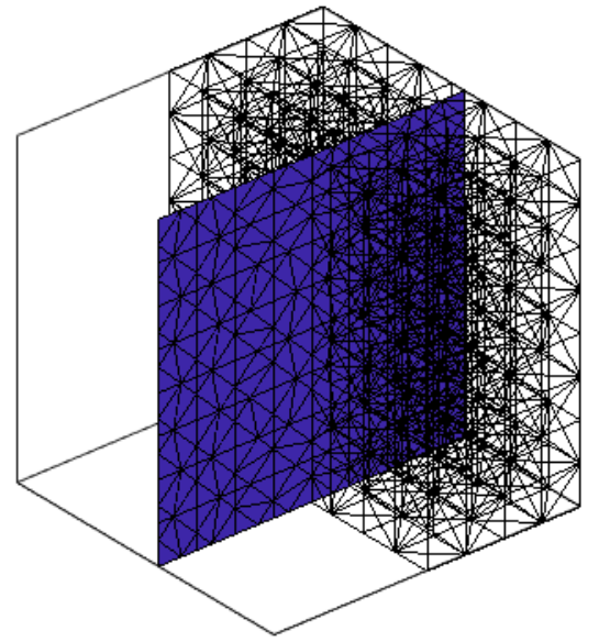
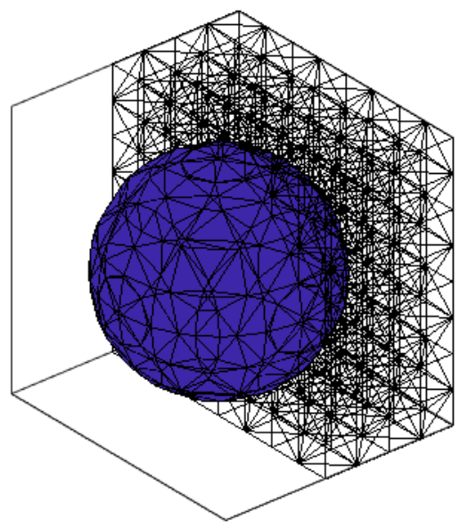
Refer to caption
Refer to caption
Refer to caption
Figure 6.1: Interface shapes: flat interface (left), a spheric interface (middle) and a torus interface (right).

6.1 Test 1(Stability)

In the first test, we study the numerical stability of the method with respect to mesh size and interface location. We first provide a group of numerical estimates for the quantity ηs\eta_{s} in (4.9) indicating a lower bound of the inf-sup constant. We consider the spheric interface shape shown in the middle plot of Figure 6.1 for the three groups of parameters.

(max⁡(β+,β−)min⁡(β+,β−),max⁡(α+,α−)min⁡(α+,α−))=(200,100),(200,1000),(2000,100)\begin{split}\left(\frac{\max(\beta^{+},\beta^{-})}{\min(\beta^{+},\beta^{-})},~~\frac{\max(\alpha^{+},\alpha^{-})}{\min(\alpha^{+},\alpha^{-})}\right)=(200,100),(200,1000),(2000,100)\end{split} (6.1)

where the minimal values are always set as 11, see the detailed parameter illustration in the right corner of plots in Figure 6.2. Then, we consider a sequence of meshes with N=10,20,30,40,50,60,70N=10,20,30,40,50,60,70. We plot the values of ηs\eta_{s} in Figure 6.2. Here, the computational results for the first two groups of parameters are presented in the first two plots, but for the third group, we separate the parameter (β+,α−)=(2000,100)(\beta^{+},\alpha^{-})=(2000,100) in a single plot to show more details. Overall, we can see that ηs\eta_{s} is bounded below. More specifically, we can make the following numerical observations:

  • •

    ηs\eta_{s} slightly decreases at the beginning, and then the curve proceeds to be flat as the mesh becomes finer.

  • •

    ηs\eta_{s} highly depends on the contrast of the parameters, and the larger contrast leads to smaller ηs\eta_{s}. Particularly, the values decrease from the first to the third group of parameters.

  • •

    Furthermore, for the third group that the parameters have the ratio (2000,100)(2000,100), when (α−,β+)=(100,2000)(\alpha^{-},\beta^{+})=(100,2000), ηs≈2.6×10⁻³\eta_{s}\approx 2.6\times 10^{-3} for the mesh N=20N=20, which is indeed close to zero. But it turns back to around 0.050.05 for finer meshes.

These observations are consistent with the analysis (cf. [39]) that the inf-sup condition only holds for sufficiently small mesh size.

Figure 6.2: Estimates of ηs\eta_{s} for various α\alpha, β\beta and mesh size.

Next, we test the condition number of 𝐁P​G{\bf B}^{PG} with respect to various interface locations. Consider a flat interface (𝐱−𝐱0)⋅𝐧=0({\bf x}-{\bf x}_{0})\cdot{\bf n}=0 passing through 𝐱0=[ϵ,0,0]{\bf x}_{0}=[\epsilon,0,0] with ϵ=10−j\epsilon=10^{-j}, j=1,2,…,6j=1,2,...,6 and the normal vector 𝐧=[1,0,0]⊤{\bf n}=[1,0,0]^{\top} such that the interface gradually moves to one face/edge of interface elements. Thus the small subelements exist for every interface element. The condition numbers are shown in Table 2 for various ϵ\epsilon. In fact, as the interface element shrinks to a non-interface element, the IFE functions will converge to standard FE functions which is “good” for computation.

ϵ\epsilon 10−110^{-1} 10−210^{-2} 10−310^{-3} 10−410^{-4} 10−510^{-5} 10−610^{-6}
cond(𝐁P​G{\bf B}^{PG}) 88267 83052 78834 84570 78253 81324
Table 2: Condition numbers for the flat interface with various ϵ\epsilon.

6.2 Example 2 (Optimal Convergence)

In the second test, we investigate the optimal convergence rates with respect to mesh size and speed of the fast solver. Consider a spheric interface with a radius r1r_{1} shown in the left plot of Figure 6.1. We still employ (1.3) as the model equation, and use the benchmark example from [39] of which the analytical solution is given by

𝐮={1β−​𝐱+1α−​n1​R1​(𝐱)​[(x2−x3),(x3−x1),(x1−x2)]⊤in​Ω−,1β+​𝐱+1α+​n2​R1​(𝐱)​R2​(𝐱)​[(x2−x3),(x3−x1),(x1−x2)]⊤in​Ω+,{\bf u}=\begin{cases}&\frac{1}{\beta^{-}}{\bf x}+\frac{1}{\alpha^{-}}n_{1}R_{1}({\bf x})[(x_{2}-x_{3}),(x_{3}-x_{1}),(x_{1}-x_{2})]^{\top}~~~~~~~~~~~~\text{in}~\Omega^{-},\\ &\frac{1}{\beta^{+}}{\bf x}+\frac{1}{\alpha^{+}}n_{2}R_{1}({\bf x})R_{2}({\bf x})[(x_{2}-x_{3}),(x_{3}-x_{1}),(x_{1}-x_{2})]^{\top}~~~~\text{in}~\Omega^{+},\end{cases} (6.2)

where 𝐱=[x1,x2,x3]⊤{\bf x}=[x_{1},x_{2},x_{3}]^{\top}, R1​(𝐱)=r12−‖𝐱‖2R_{1}({\bf x})=r^{2}_{1}-\|{\bf x}\|^{2}, R2​(𝐱)=r22−‖𝐱‖2R_{2}({\bf x})=r^{2}_{2}-\|{\bf x}\|^{2}, and n1=n2​(r22−r12)n_{1}=n_{2}(r^{2}_{2}-r^{2}_{1}). We let (α−,α+)=(β−,β+)=(1,100)(\alpha^{-},\alpha^{+})=(\beta^{-},\beta^{+})=(1,100) and (1,1000)(1,1000), and denote ρ=α+/α−=β+/β−\rho=\alpha^{+}/\alpha^{-}=\beta^{+}/\beta^{-}. We present the numerical results for N=10,…,70N=10,...,70 in Figure 6.3 which clearly show the optimal convergence rates.

To solve the linear system, we employ the preconditioner described in Section 4.2 with both GMRES and CG iteration strategies. Of course, it involves a direct solver on a smaller matrix of which the size depends on the expanding width ll, i.e., the size of 𝐁l(2,2){\bf B}^{(2,2)}_{l} in (4.4). But the block diagonal smoother in (4.7) can help in greatly reducing the iteration steps for convergence, and consequently significantly reduce the computational time. In fact, as ll is small, in practice we store the L​ULU factorization of 𝐁l(2,2){\bf B}^{(2,2)}_{l} to avoid repeatly compute the inverse. In Table 3, we present both the number of iterations and computational time for GMRES. It is highlighted that the preconditioning strategy even works for a CG method which in general does not converge for non-SPD matrices. The resuls are presented in Table 4, and we can observe that the CG method must need l=1l=1 at least for convergence. But once the block diagonal smoother in (4.7) is used, the CG method has better performance than GMRES. We may refer to our detailed discussions in Section 4.2, and point out again the important fact that the majority portion of 𝐁P​G{\bf B}^{PG} is symmetric, and the problematic portion is only around the interface which can be well-handled by the direct inverse (𝐁l(2,2))−1({\bf B}^{(2,2)}_{l})^{-1}. Overall, for both methods we observe that the expanding width ll depends on the contrast ρ\rho. For a larger contrast, there needs a relatively larger ll to ensure fast convergence. With an appropriately chosen expanding width, the algorithm converges in a small number of iterations which indeed takes significantly less computational time.

(a) OPENα−,α+)=(β−,β+)=(1,100)\alpha^{-},\alpha^{+})=(\beta^{-},\beta^{+})=(1,100)
(b) (α−,α+)=(β−,β+)=(1,1000)(\alpha^{-},\alpha^{+})=(\beta^{-},\beta^{+})=(1,1000)
Figure 6.3: Errors for Example 2 where the dashed line is the reference line indicating 𝒪⁡(h)\mathcal{O}(h).
# DoFs 79307930 5966059660 197190197190 462520462520 897650897650 15445801544580 24453102445310
ρ=100\rho=100, l=0l=0 63(2.63s) 66(14s) 66(29s) 67(51s) 68(108s) 68(191s) 68(283s)
ρ=100\rho=100, l=1l=1 35(2.11s) 40(7.89s) 39(14s) 40(28s) 40(56s) 38(100s) 41(147s)
ρ=1000\rho=1000, l=0l=0 212(8.87s) 244(60s) 263(117s) 223(185s) 246(404s) 272(817s) 234(1017s)
ρ=1000\rho=1000, l=1l=1 55(8.44s) 63(13.67s) 76(33s) 48(35s) 46(70s) 52(143s) 54(243s)
ρ=1000\rho=1000, l=2l=2 42(1.9s) 47(11.23s) 46(21s) 52(39s) 46(83s) 51(144s) 51(209s)
ρ=1000\rho=1000, l=3l=3 41(32s) 39(11s) 42(20s) 39(40s) 42(75s) 42(135s) 42(191s)
Table 3: Iteration numbers and computational time for the GMRES solver.
# DoFs 79307930 5966059660 197190197190 462520462520 897650897650 15445801544580 24453102445310
ρ=100\rho=100, l=0l=0 – 84(18s) 78(29s) – – – –
ρ=100\rho=100, l=1l=1 37(1.6s) 39(9.8s) 40(18s) 41(30s) 42(56s) 42(99s) 43(140s)
ρ=100\rho=100, l=2l=2 36(1.3s) 39(10s) 41(17s) 42(32s) 42(66s) 42(110s) 42(170s)
ρ=1000\rho=1000, l=0l=0 – – – – – – –
ρ=1000\rho=1000, l=1l=1 40(1.4s) 42(17s) 42(30s) 42(30s) 43(59s) 45(100s) 43(140s)
ρ=1000\rho=1000, l=2l=2 37(1.4s) 39(8.4s) 40(18s) 41(29s) 42(61s) 44(110s) 42(150s)
Table 4: Iteration numbers and computational time for the CG solver.

6.3 Example 3 (Application to a time-domain Maxwell equation)

In this test, we consider the scattering problem modeled by (1.2) in a time domain [0,T][0,T]. We partition it into MM sub-intervals: t0=0<t1<t2<⋯<tM=Tt_{0}=0<t_{1}<t_{2}<\cdots<t_{M}=T with equal length τ=T/M\tau=T/M. We then apply the implicit time-discretization introduced in [29] which reads

(ϵ​∂τ2𝐮hn,𝐯h)Ω+(σ​∂τ𝐮hn,𝐯h)Ω+(μ−1​curl⁡𝐮hn,curl⁡𝐯h)Ω=(𝐉t,𝐯h)Ω,∀𝐯h∈𝐒he,(\epsilon\partial^{2}_{\tau}{\bf u}^{n}_{h},{\bf v}_{h})_{\Omega}+(\sigma\partial_{\tau}{\bf u}^{n}_{h},{\bf v}_{h})_{\Omega}+(\mu^{-1}\operatorname{curl}{\bf u}^{n}_{h},\operatorname{curl}{\bf v}_{h})_{\Omega}=({\bf J}_{t},{\bf v}_{h})_{\Omega},~~~~\forall{\bf v}_{h}\in{\bf S}^{e}_{h}, (6.3)

where, for n≥2n\geq 2, ∂τ𝐮hn=(𝐮hn−𝐮hn−1)/τ\partial_{\tau}{\bf u}^{n}_{h}=({\bf u}^{n}_{h}-{\bf u}^{n-1}_{h})/\tau and ∂τ2𝐮hn=(∂τ𝐮hn−∂τ𝐮hn−1)/τ\partial^{2}_{\tau}{\bf u}^{n}_{h}=(\partial_{\tau}{\bf u}^{n}_{h}-\partial_{\tau}{\bf u}^{n-1}_{h})/\tau. Then, at each time step it can be discretized by the PG-IFE scheme with the parameters α=μ−1\alpha=\mu^{-1} and β=ϵ​τ−2+σ​τ−1\beta=\epsilon\tau^{-2}+\sigma\tau^{-1} and solved with the proposed fast solver. The optimal convergence rates can be also observed if the analytical solution is available, which is omitted for avoiding redundancy. Here, we consider a simulation problem of electromagnetic waves propagating through a torus where the analytical solution is difficult to derive if not impossible, but instead we compare the results of the IFE method and the standard FE method on fitted meshes.

The torus interface shown in the right plot of Figure 6.1 is described by a level-set signed-distance function:

γ⁡(𝐱)=((x1−z1)2+(x2−z2)2−r2)2+(x3−z3)2−r12,\gamma({\bf x})=(\sqrt{(x_{1}-z_{1})^{2}+(x_{2}-z_{2})^{2}}-r_{2})^{2}+(x_{3}-z_{3})^{2}-r_{1}^{2},

where z1=z2=0z_{1}=z_{2}=0, z3=−0.3z_{3}=-0.3 and r1=0.2r_{1}=0.2, r2=π/5r_{2}=\pi/5. We further set the medium parameters as ϵ+=0.05\epsilon^{+}=0.05, ϵ−=2​ϵ+\epsilon^{-}=2\epsilon^{+}, σ+=0.1\sigma^{+}=0.1, σ−=1\sigma^{-}=1 and μ+=4​π\mu^{+}=4\pi, μ−=3​μ+\mu^{-}=3\mu^{+}. Initially, we impose a Gaussian pulse

𝐮=exp⁡(−b​(a⁡(x1−z0)−ω​t)2)​[0,1,0]⊤{\bf u}=\exp(-b(a(x_{1}-z_{0})-\omega t)^{2})[0,1,0]^{\top} (6.4)

where a=ω​ϵ+​μ+a=\omega\sqrt{\epsilon^{+}\mu^{+}} modeling the speed of the electromagnetic wave. In addition, the boundary condition is set to match (6.4) except on the faces at 𝐱=−1,1{\bf x}=-1,1 where it is set as 𝟎\mathbf{0}. Set the source as 𝐉=𝟎{\bf J}=\mathbf{0}, let the time domain be [0,1.5][0,1.5] and let the step size be τ=1.5/128\tau=1.5/128. The IFE method is computed on a 64364^{3} unfitted mesh which contains 1572864 elements and 1872064 DoFs, while the simulation of the FE method is performed on a fitted mesh containing 1679542 elements and 2002947 DoFs.

Denote the numerical solutions by 𝐮hI​F​E{\bf u}^{IFE}_{h} and 𝐮hF​E{\bf u}^{FE}_{h}, respectively. To compare the simulation results, we first plot the evolution of the x2x_{2} component at some slices in Figure 6.4 at t=12​τt=12\tau, t=24​τt=24\tau, t=36​τt=36\tau and t=48​τt=48\tau. The results of the IFE and FE methods are almost identical demonstrating the effectiveness of the proposed method. In addition, we can clearly observe the delayed electromagnetic wave inside the torus agreeing with the physics. Next, we plot the electromagnetic fields inside the torus in Figure 6.5 such that we can also examine the direction. The plots still clearly show that the two methods have very similar simulation results.

t=12​τt=12\tau t=24​τt=24\tau t=36​τt=36\tau t=48​τt=48\tau
Refer to caption Refer to caption Refer to caption Refer to caption
Figure 6.4: Comparison of FE (top) and IFE (bottom) solutions at slices x1=5/32x_{1}=5/32, x2=5/16x_{2}=5/16, x3=−5/16x_{3}=-5/16.
t=12​τt=12\tau t=24​τt=24\tau t=36​τt=36\tau t=48​τt=48\tau
Refer to caption Refer to caption Refer to caption Refer to caption
Figure 6.5: Comparison of FE (top) and IFE (bottom) solutions of vector fields.

Appendix A Proof of Lemma 1

Here, we only show (2.3b), since it can yield (2.3a) by the argument in [38]. Since φΓ\varphi^{\Gamma} is sufficiently smooth, we obtain by the interpolation approximation that

‖∇φΓ−∇φhΓ‖L∞​(K)≤C​hK\|\nabla\varphi^{\Gamma}-\nabla\varphi^{\Gamma}_{h}\|_{L^{\infty}(K)}\leq Ch_{K} (A.1)

where CC depends on the second derivative of φΓ\varphi^{\Gamma}. As a signed-distance function, φΓ\varphi^{\Gamma} satisfies ‖∇φΓ‖=1\|\nabla\varphi^{\Gamma}\|=1, and thus (A.1) implies

|1−‖∇φhΓ​(𝐱)‖|≤C​hK,∀𝐱∈K.{\left|1-\|\nabla\varphi^{\Gamma}_{h}({\bf x})\|\right|}\leq Ch_{K},~~~\forall{\bf x}\in K. (A.2)

Note that the unit normal vectors of Γ\Gamma and ΓhK\Gamma^{K}_{h} are ∇φΓ\nabla\varphi^{\Gamma} and ∇φhΓ/‖∇φhΓ‖\nabla\varphi^{\Gamma}_{h}/\|\nabla\varphi^{\Gamma}_{h}\|, respectively. Then, for sufficiently small hh, (A.1) and (A.2) together yield

‖∇φΓ−∇φhΓ/‖∇φhΓ‖‖L∞​(K)≤‖∇φΓ−∇φhΓ+∇φΓ​(‖∇φhΓ‖−1)‖L∞​(K)min𝐱∈K⁡‖∇φhΓ​(𝐱)‖≲hK\|\nabla\varphi^{\Gamma}-\nabla\varphi^{\Gamma}_{h}/\|\nabla\varphi^{\Gamma}_{h}\|\|_{L^{\infty}(K)}\leq\frac{\|\nabla\varphi^{\Gamma}-\nabla\varphi^{\Gamma}_{h}+\nabla\varphi^{\Gamma}(\|\nabla\varphi^{\Gamma}_{h}\|-1)\|_{L^{\infty}(K)}}{\min_{{\bf x}\in K}\|\nabla\varphi^{\Gamma}_{h}({\bf x})\|}\lesssim h_{K}

which has finished the proof.

Appendix B Proof of Lemma 12

Here, we only prove (5.9a) with d=curl\,{\rm d}=\operatorname{curl}, i.e., a=1a=1, and the others are similar. Let 𝐯=𝐮E−×𝐧¯K−𝐮E+×𝐧¯K{\bf v}={\bf u}^{-}_{E}\times\bar{{\bf n}}_{K}-{\bf u}^{+}_{E}\times\bar{{\bf n}}_{K}. Without loss of generality, we define a local system (x^1,x^2,x^3)(\hat{x}_{1},\hat{x}_{2},\hat{x}_{3}) with x^3\hat{x}_{3} being the direction normal to ΓhωK\Gamma^{\omega_{K}}_{h}, i.e., 𝐧¯K\bar{{\bf n}}_{K}, and x^1,x^2\hat{x}_{1},\hat{x}_{2} spanning the plane containing ΓhωK\Gamma^{\omega_{K}}_{h} such that the interface surface can be represented by x^3=f⁡(x^1,x^2)\hat{x}_{3}=f(\hat{x}_{1},\hat{x}_{2}) with ff being a smooth function. Then,

𝐯⁡(x^1,x^2,f⁡(x^1,x^2))=𝐯⁡(x^1,x^2,0)+∫0f⁡(x^1,x^2)∂x^3𝐯⁡(x^1,x^2,x^3)​d​x^3{\bf v}(\hat{x}_{1},\hat{x}_{2},f(\hat{x}_{1},\hat{x}_{2}))={\bf v}(\hat{x}_{1},\hat{x}_{2},0)+\int_{0}^{f(\hat{x}_{1},\hat{x}_{2})}\partial_{\hat{x}_{3}}{\bf v}(\hat{x}_{1},\hat{x}_{2},\hat{x}_{3})\,{\rm d}\hat{x}_{3} (B.1)

which, by Hölder’s inequality, yields

‖𝐯‖L2​(ΓhωK)2=∫ΓhωK‖𝐯⁡(x^1,x^2,0)‖2​d​x^1​d​x^2≲∫ΓhωK‖𝐯⁡(x^1,x^2,f⁡(x^1,x^2))‖2​d​x^1​d​x^2+∫ΓhωK∫0f⁡(x^1,x^2)∥∂x^3𝐯(x^1,x^2,f(x^1,x^2))∥2dx^3|f(x^1,x^2)|dx^1dx^2\begin{split}\|{\bf v}\|^{2}_{L^{2}(\Gamma^{\omega_{K}}_{h})}&=\int_{\Gamma^{\omega_{K}}_{h}}\|{\bf v}(\hat{x}_{1},\hat{x}_{2},0)\|^{2}\,{\rm d}\hat{x}_{1}\,{\rm d}\hat{x}_{2}\lesssim\int_{\Gamma^{\omega_{K}}_{h}}\|{\bf v}(\hat{x}_{1},\hat{x}_{2},f(\hat{x}_{1},\hat{x}_{2}))\|^{2}\,{\rm d}\hat{x}_{1}\,{\rm d}\hat{x}_{2}\\ &+\int_{\Gamma^{\omega_{K}}_{h}}\int_{0}^{f(\hat{x}_{1},\hat{x}_{2})}\|\partial_{\hat{x}_{3}}{\bf v}(\hat{x}_{1},\hat{x}_{2},f(\hat{x}_{1},\hat{x}_{2}))\|^{2}\,{\rm d}\hat{x}_{3}|f(\hat{x}_{1},\hat{x}_{2})|\,{\rm d}\hat{x}_{1}\,{\rm d}\hat{x}_{2}\end{split} (B.2)

of which the last two integrals are denoted by (I)({\rm I}) and (II)({\rm II}), respectively. With (5.8), it is clear that

(II)≤max(x^1,x^2)∈ΓhωK⁡|f⁡(x^1,x^2)|​‖∂x^3𝐯‖L2​(ωK)2≲hK2​‖∇𝐯‖L2​(ωK)2.({\rm II})\leq\max_{(\hat{x}_{1},\hat{x}_{2})\in\Gamma^{\omega_{K}}_{h}}|f(\hat{x}_{1},\hat{x}_{2})|\|\partial_{\hat{x}_{3}}{\bf v}\|^{2}_{L^{2}(\omega_{K})}\lesssim h^{2}_{K}\|\nabla{\bf v}\|^{2}_{L^{2}(\omega_{K})}. (B.3)

As for (I)({\rm I}), we note that 1+‖∇f‖2≥1\sqrt{1+\|\nabla f\|^{2}}\geq 1, and thus obtain

(I)≤∫ΓhωK‖𝐯⁡(x^1,x^2,f⁡(x^1,x^2))‖2​1+‖∇f‖2​d​x^1​d​x^2=∫ΓωK‖𝐯‖2​𝑑s=‖𝐯‖L2​(ΓωK)2=‖(𝐮E−−𝐮E+)×(𝐧−𝐧¯K)‖L2​(ΓωK)2≲maxΓωK⁡‖𝐧−𝐧¯K‖2​‖𝐮E−−𝐮E+‖L2​(ΓωK)2≲hK2​‖𝐮‖E,1,ωK\begin{split}({\rm I})&\leq\int_{\Gamma^{\omega_{K}}_{h}}\|{\bf v}(\hat{x}_{1},\hat{x}_{2},f(\hat{x}_{1},\hat{x}_{2}))\|^{2}\sqrt{1+\|\nabla f\|^{2}}\,{\rm d}\hat{x}_{1}\,{\rm d}\hat{x}_{2}=\int_{\Gamma^{\omega_{K}}}\|{\bf v}\|^{2}\,{\rm d}s=\|{\bf v}\|^{2}_{L^{2}(\Gamma^{\omega_{K}})}\\ &=\|({\bf u}^{-}_{E}-{\bf u}^{+}_{E})\times({\bf n}-\bar{{\bf n}}_{K})\|^{2}_{L^{2}(\Gamma^{\omega_{K}})}\lesssim\max_{\Gamma^{\omega_{K}}}\|{\bf n}-\bar{{\bf n}}_{K}\|^{2}\|{\bf u}^{-}_{E}-{\bf u}^{+}_{E}\|^{2}_{L^{2}(\Gamma^{\omega_{K}})}\\ &\lesssim h^{2}_{K}\|{\bf u}\|_{E,1,\omega_{K}}\end{split} (B.4)

where we have used (𝐮E−−𝐮E+)×𝐧=0({\bf u}^{-}_{E}-{\bf u}^{+}_{E})\times{\bf n}=0 on ΓωK\Gamma^{\omega_{K}}, (5.8) and the trace inequality from Lemma 3.1 in [64].

Refer to caption
Refer to caption
Figure B.1: Two types of interface-cutting configuration for a regular tetrahedron. Left (Case 1): 3 intersection points and right (Case 2): 4 intersection points.

Appendix C Proof of Lemma 2 for a regular tetrahedron

We treat the cases of 3 or 4 intersection points shown in Figure B.1, separatly, where DiD_{i} are the intersection points of the approximate interface ΓhK\Gamma^{K}_{h} with the edges. Without loss of generality, we assume the tetrahedron has the vertices A1​(0,0,0)A_{1}(0,0,0), A2​(1,0,0)A_{2}(1,0,0), A3​(1/2,3/2,0)A_{3}(1/2,\sqrt{3}/2,0), A4​(1/2,3/6,6/3)A_{4}(1/2,\sqrt{3}/6,\sqrt{6}/3). The three faces are chosen as A1​A2​A3A_{1}A_{2}A_{3}, A1​A3​A4A_{1}A_{3}A_{4} and A1​A2​A4A_{1}A_{2}A_{4}. In addition, for Case 1 we let the intersection points be D1=d1​A2D_{1}=d_{1}A_{2}, D2=d2​A3D_{2}=d_{2}A_{3}, D3=d3​A4D_{3}=d_{3}A_{4}, and for Case 2 we let them be D1=d1​A2D_{1}=d_{1}A_{2}, D2=d2​A3D_{2}=d_{2}A_{3}, D3=(1−d3)​A4+d3​A3D_{3}=(1-d_{3})A_{4}+d_{3}A_{3} and D4=(1−d4)​A4+d4​A2D_{4}=(1-d_{4})A_{4}+d_{4}A_{2}, where di∈[0,1]d_{i}\in[0,1], i=1,2,3,4i=1,2,3,4, are parameters of their location. For Case 2, since DiD_{i} are coplanar, d4d_{4} can be expressed as

d4=d1​d3​(d2−1)d1​d2+d2​d3−d2−d1​d3.d_{4}=\frac{d_{1}d_{3}(d_{2}-1)}{d_{1}d_{2}+d_{2}d_{3}-d_{2}-d_{1}d_{3}}. (C.1)

We use Mathematica to express the determinant as

det​(MK)=f1​(d1,d2,d3)+f2​(d1,d2,d3)​α~+f3​(d1,d2,d3)​α~2f0​(d1,d2,d3)\text{det}(M_{K})=\frac{f_{1}(d_{1},d_{2},d_{3})+f_{2}(d_{1},d_{2},d_{3})\tilde{\alpha}+f_{3}(d_{1},d_{2},d_{3})\tilde{\alpha}^{2}}{f_{0}(d_{1},d_{2},d_{3})} (C.2)

where fi​(d1,d2,d3)f_{i}(d_{1},d_{2},d_{3}), i=0,1,2,3i=0,1,2,3, are some polynomials of d1,d2,d3d_{1},d_{2},d_{3}. We omit the explicit formulas for the functions fif_{i} here since they are complicated. When α~=1\tilde{\alpha}=1, i.e., AK=IA_{K}=I, it is straightforward to calculate det(MK)=−1/16\text{det}(M_{K})=-1/16, and thus

f1​(d1,d2,d3)+f2​(d1,d2,d3)+f3​(d1,d2,d3)=−116​f0​(d1,d2,d3).f_{1}(d_{1},d_{2},d_{3})+f_{2}(d_{1},d_{2},d_{3})+f_{3}(d_{1},d_{2},d_{3})=-\frac{1}{16}f_{0}(d_{1},d_{2},d_{3}). (C.3)

For Case 1, we can verify that fi(d1,d2,d3)≤0,i=1,2,3f_{i}(d_{1},d_{2},d_{3})\leq 0,~i=1,2,3 and f0​(d1,d2,d3)≥0f_{0}(d_{1},d_{2},d_{3})\geq 0. Thus, by (C.3) we have

f1​(d1,d2,d3)+f2​(d1,d2,d3)​α~+f3​(d1,d2,d3)​α~2≤min⁡{α~2,1}​∑i=1,2,3fi​(d1,d2,d3)=−min⁡{α~2,1}16​f0​(d1,d2,d3).\begin{split}&f_{1}(d_{1},d_{2},d_{3})+f_{2}(d_{1},d_{2},d_{3})\tilde{\alpha}+f_{3}(d_{1},d_{2},d_{3})\tilde{\alpha}^{2}\\ \leq&\min\{\tilde{\alpha}^{2},1\}\sum_{i=1,2,3}f_{i}(d_{1},d_{2},d_{3})=-\frac{\min\{\tilde{\alpha}^{2},1\}}{16}f_{0}(d_{1},d_{2},d_{3}).\end{split} (C.4)

For Case 2, we can veriify that fi(d1,d2,d3)≥0,i=1,2,3f_{i}(d_{1},d_{2},d_{3})\geq 0,~i=1,2,3 and f0​(d1,d2,d3)≤0f_{0}(d_{1},d_{2},d_{3})\leq 0. Similar to (C.4), we obtain

f1​(d1,d2,d3)+f2​(d1,d2,d3)​α~+f3​(d1,d2,d3)​α~2≥−min⁡{α~2,1}16​f0​(d1,d2,d3).f_{1}(d_{1},d_{2},d_{3})+f_{2}(d_{1},d_{2},d_{3})\tilde{\alpha}+f_{3}(d_{1},d_{2},d_{3})\tilde{\alpha}^{2}\geq-\frac{\min\{\tilde{\alpha}^{2},1\}}{16}f_{0}(d_{1},d_{2},d_{3}). (C.5)

Combining (C.4) and (C.4), for both cases we arrive at

det​(MK)≤−min⁡{α~2,1}16<0.\text{det}(M_{K})\leq-\frac{\min\{\tilde{\alpha}^{2},1\}}{16}<0. (C.6)

References

  • [1] R. Albanese and P. B. Monk, The inverse source problem for Maxwell’s equations, Inverse Problems, 22 (2006), pp. 1023–1035.
  • [2] H. Ammari, G. Bao, and J. L. Fleming, An inverse source problem for Maxwell’s equations in magnetoencephalography, SIAM J. Appl. Math., 62 (2002).
  • [3] H. Ammari, J. Chen, Z. Chen, D. Volkov, and H. Wang, Detection and classification from electromagnetic induction data, J. Comput. Phys., 301 (2015), pp. 201 – 217.
  • [4] L. B. ao da Veiga, F. Dassi, G. Manzini, and L. Mascotto, Virtual elements for maxwell’s equations, Comput. Math. Appl., (2021).
  • [5] D. N. Arnold, R. S. Falk, and R. Winther, Preconditioning in H(div) and applications, Math. Comp., 66 (1997).
  • [6] I. Babuška, G. Caloz, and J. E. Osborn, Special finite element methods for a class of second order elliptic problems with rough coefficients, SIAM J. Numer. Anal., 31 (1994), pp. 945–981.
  • [7] K. Bathe, The inf–sup condition and its evaluation for mixed finite element methods, Computers & Structures, 79 (2001), pp. 243–252.
  • [8] R. Becker, E. Burman, and P. Hansbo, A Nitsche extended finite element method for incompressible elasticity with discontinuous modulus of elasticity, Comput. Methods Appl. Mech. Engrg., 198 (2009), pp. 3352–3360.
  • [9] F. Ben Belgacem, A. Buffa, and Y. Maday, The mortar finite element method for 3d Maxwell equations: First results, SIAM J. Numer. Anal., 39 (2001), pp. 880–901.
  • [10] J. R. Brauer, J. J. Ruehl, M. A. Juds, M. J. V. Heiden, and A. A. Arkadan, Dynamic stress in magnetic actuator computed by coupled structural and electromagnetic finite elements, IEEE Trans. Magn., 32 (1996).
  • [11] S. C. Brenner, J. Cui, F. Li, and L. Y. Sung, A nonconforming finite element method for a two-dimensional curl–curl and grad-div problem, Numer. Math., 109 (2008), pp. 509–533.
  • [12] A. Buffa, M. Costabel, and M. Dauge, Algebraic convergence for anisotropic edge elements in polyhedral domains, Numer. Math., 101 (2005), pp. 29–65.
  • [13] E. Burman, S. Claus, P. Hansbo, M. G. Larson, and A. Massing, CutFEM: Discretizing geometry and partial differential equations, Internat. J. Numer. Methods Engrg., 104 (2015), pp. 472–501.
  • [14] E. Burman, J. Guzmán, M. A. Sánchez, and M. Sarkis, Robust flux error estimation of an unfitted nitsche method for high-contrast interface problems, IMA J. Numer. Anal., 38 (2018), pp. 646–668.
  • [15] Z. Cai and S. Cao, A recovery-based a posteriori error estimator for H(curl) interface problems, Comput. Methods Appl. Mech. Engrg., 296 (2015), pp. 169 – 195.
  • [16] S. Cao and L. Chen, Anisotropic error estimates of the linear virtual element method on polygonal meshes, SIAM J. Numer. Anal., 56 (2018), pp. 2913–2939.
  • [17] S. Cao, L. Chen, and R. Guo, A virtual finite element method for two dimensional Maxwell interface problems with a background unfitted mesh, Math. Models Methods Appl. Sci., 31 (2021), pp. 2907–2936.
  • [18]  , Immersed virtual element methods for Maxwell interface problems in three dimensions, ArXiv preprint, (2022).
  • [19] R. Casagrande, R. Hiptmair, and J. Ostrowski, An a priori error estimate for interior penalty discretizations of the curl-curl operator on non-conforming meshes, J. Math. Ind., 6 (2016), p. 4.
  • [20] R. Casagrande, C. Winkelmann, R. Hiptmair, and J. Ostrowski, DG treatment of non-conforming interfaces in 3D Curl-Curl problems, in Scientific Computing in Electrical Engineering, Cham, 2016, Springer International Publishing, pp. 53–61.
  • [21] D. Chapelle and K. Bathe, The inf-sup test, Computers & Structures, 47 (1993), pp. 537–545.
  • [22] J. Chen, Y. Liang, and J. Zou, Mathematical and numerical study of a three-dimensional inverse eddy current problem, SIAM J. Appl. Math., 80 (2020), pp. 1467–1492.
  • [23] L. Chen, iifem: an integrated finite element methods package in MATLAB, tech. rep., 2009.
  • [24] L. Chen, H. Wei, and M. Wen, An interface-fitted mesh generator and virtual element methods for elliptic interface problems, J. Comput. Phys., 334 (2017), pp. 327–348.
  • [25] Z. Chen, Q. Du, and J. Zou, Finite element methods with matching and nonmatching meshes for Maxwell equations with discontinuous coefficients, SIAM J. Numer. Anal., 37 (2000), pp. 1542–1570.
  • [26] Z. Chen, L. Wang, and W. Zheng, An adaptive multilevel method for time‐harmonic Maxwell equations with singularities, SIAM J. Sci. Comput., 29 (2007), pp. 118–138.
  • [27] Z. Chen, Y. Xiao, and L. Zhang, The adaptive immersed interface finite element method for elliptic and Maxwell interface problems, J. Comput. Phys., 228 (2009), pp. 5000 – 5019.
  • [28] C.-C. Chu, I. G. Graham, and T.-Y. Hou, A new multiscale finite element method for high-contrast elliptic interface problems, Math. Comp., 79 (2010), pp. 1915–1955.
  • [29] P. Ciarlet, Jr and J. Zou, Fully discrete finite element approaches for time-dependent Maxwell’s equations, Numer. Math., 82 (1999), pp. 193–219.
  • [30] M. Costabel and M. Dauge, Singularities of electromagnetic fields in polyhedral domains, Arch. Ration. Mech. Anal., 151 (2000), pp. 221–276.
  • [31] M. Costabel, M. Dauge, and S. Nicaise, Singularities of Maxwell interface problems., ESAIM: M2AN, 33 (1999), pp. 627–649.
  • [32]  , Corner Singularities of Maxwell Interface and Eddy Current Problems, Birkhäuser Basel, Basel, 2004, pp. 241–256.
  • [33] L. B. da Veiga and L. Mascotto, Interpolation and stability properties of low order face and edge virtual element spaces, IMA J. Numer. Anal., (2022).
  • [34] E. M. Dede, J. Lee, and T. Nomura, Multiphysics Simulation: Electromechanical System Applications and Optimization, Springer, 2014.
  • [35] H. Edelsbrunner, Triangulations and meshes in computational geometry, Acta Numerica, 9 (2000), pp. 133–213.
  • [36] S. Groß and A. Reusken, An extended pressure finite element space for two-phase incompressible flows with surface tension, J. Comput. Phys., 224 (2007), pp. 40 – 58. Special Issue Dedicated to Professor Piet Wesseling on the occasion of his retirement from Delft University of Technology.
  • [37] R. Guo, Solving parabolic moving interface problems with dynamical immersed spaces on unfitted meshes: Fully discrete analysis, SIAM J. Numer. Anal., 2 (2021), pp. 797–828.
  • [38] R. Guo and T. Lin, An immersed finite element method for elliptic interface problems in three dimensions, J. Comput. Phys., 414 (2020).
  • [39] R. Guo, Y. Lin, and J. Zou, Solving two dimensional H(curl)-elliptic interface systems with optimal convergence on unfitted meshes, arXiv:2011.11905, (2020).
  • [40] R. Guo, Y. L. T. Lin, and Q. Zhuang, Error analysis of symmetric linear/bilinear partially penalized immersed finite element methods for helmholtz interface problems, J. Comput. Appl. Math., (2021).
  • [41] P. Hansbo, M. G. Larson, and S. Zahedi, A cut finite element method for a stokes interface problem, Appl. Numer. Math., 85 (2014), pp. 90–114.
  • [42] R. Hiptmair, J. LI, and J. Zou, Convergence analysis of finite element methods for H⁡(d​i​v,Ω){H}(div;{\Omega})-elliptic interface problems, J. Numer. Math., 18 (2010), pp. 187–218.
  • [43] R. Hiptmair, J. Li, and J. Zou, Convergence analysis of finite element methods for H(curl; Ω\Omega)-elliptic interface problems, Numer. Math., 122 (2012), pp. 557–578.
  • [44] R. Hiptmair, A. Moiola, and I. Perugia, Stability results for the time-harmonic Maxwell equations with impedance boundary conditions, Math. Models Methods Appl. Sci., 21 (2011), pp. 2263–2287.
  • [45] R. Hiptmair and J. Xu, Nodal auxiliary space preconditioning in H(curl) and H(div) spaces, SIAM J. Numer. Anal., 45 (2007), pp. 2483–2509.
  • [46] S. Hou, P. Song, L. Wang, and H. Zhao, A weak formulation for solving elliptic interface problems without body fitted grid, J. Comput. Phys., 249 (2013), pp. 80 – 95.
  • [47] P. Houston, I. Perugia, A. Schneebeli, and D. Schötzau, Interior penalty method for the indefinite time-harmonic Maxwell equations, Numer. Math., 100 (2005), pp. 485–518.
  • [48] P. Houston, I. Perugia, and D. Schotzau, Mixed discontinuous galerkin approximation of the Maxwell operator, SIAM J. Numer. Anal., 42 (2004), pp. 434–459.
  • [49] J. Hu and H. Wang, An optimal multigrid algorithm for the combining p1p_{1}-q1q_{1} finite element approximations of interface problems based on local anisotropic fitting meshes, J. Sci. Comput., 88 (2021).
  • [50] Q. Hu, S. Shu, and J. Zou, A mortar edge element method with nearly optimal convergence for three-dimensional Maxwell’s equations, Math. Comp., 77 (2008), pp. 1333–1353.
  • [51] R. Kafafy, T. Lin, Y. Lin, and J. Wang, Three-dimensional immersed finite element methods for electric field simulation in composite materials, Internat. J. Numer. Methods Engrg., 64 (2005), pp. 940–972.
  • [52] J. Li, J. M. Melenk, B. Wohlmuth, and J. Zou, Optimal a priori estimates for higher order finite elements for elliptic interface problems, Appl. Numer. Math., 60 (2010), pp. 19–37.
  • [53] T. Lin, Y. Lin, and X. Zhang, Partially penalized immersed finite element methods for elliptic interface problems, SIAM J. Numer. Anal., 53 (2015), pp. 1121–1144.
  • [54] H. Liu, L. Zhang, X. Zhang, and W. Zheng, Interface-penalty finite element methods for interface problems in H1H^{1}, H(curl), and H(div), Comput. Methods Appl. Mech. Engrg., 367 (2020).
  • [55] G. Makinson and A. Shah, An iterative solution method for solving sparse nonsymmetric linear systems, Journal of Computational and Applied Mathematics, 15 (1986), pp. 339–352.
  • [56] P. Monk, Finite Element Methods for Maxwell’s Equations, Oxford University Press, 2003.
  • [57] J. C. Nedelec, Mixed finite elements in ℝ3\mathbb{R}^{3}, Numer. Math., 35 (1980), pp. 315–341.
  • [58] J. C. Nédélec, A new family of mixed finite elements in ℝ3\mathbb{R}^{3}, Numer. Math., 50 (1986), pp. 57–81.
  • [59] S. Osher and R. P. Fedkiw, Level set methods: An overview and some recent results, J. Comput. Phys., 169 (2001), pp. 463–502.
  • [60] P.-O. Persson and G. Strang, A simple mesh generator in Matlab, SIAM Review, 46 (2004), pp. 329–345.
  • [61] P. A. Raviart and J. M. Thomas, A mixed finite element method for 2-nd order elliptic problems, in Mathematical Aspects of Finite Element Methods, I. Galligani and E. Magenes, eds., Berlin, Heidelberg, 1977, Springer Berlin Heidelberg, pp. 292–315.
  • [62] K. Roppert, S. Schoder, F. Toth, and M. Kaltenbacher, Non-conforming nitsche interfaces for edge elements in curl–curl-type problems, IEEE Trans. Magn., 56 (2020).
  • [63] J. A. Sethian, Level set methods and fast marching methods, vol. 3 of Cambridge Monographs on Applied and Computational Mathematics, Cambridge University Press, Cambridge, second ed., 1999.
  • [64] F. Wang, Y. Xiao, and J. Xu, High-order extended finite element methods for solving interface problems, Comput. Methods Appl. Mech. Engrg., 364 (2020).
  • [65] T. Warburton and J. S. Hesthaven, On the constants in h​php-finite element trace inverse inequalities, Comput. Methods Appl. Mech. Engrg., 192 (2003), pp. 2765–2773.
  • [66] J. XU and Y. ZHU, Uniform convergent multigrid methods for elliptic problems with strongly discontinuous coefficients, Mathematical Models and Methods in Applied Sciences, 18 (2008), pp. 77–105.
  • [67] J. Xu and J. Zou, Some nonoverlapping domain decomposition methods, SIAM Review, 40 (1998), pp. 857–914.
  • [68] R. L. Z. Cai, T. A. Manteuffel, and S. F. McCormick, First-order system least squares for second-order partial differential equations: Part i, SIAM J. Numer. Anal., 31 (1994).
  • [69] S. Zhao and G. W. Wei, High-order FDTD methods via derivative matching for Maxwell’s equations with material interfaces, J. Comput. Phys., 200 (2004), pp. 60–103.