New graph-based multi-sample tests for high-dimensional and non-Euclidean data

Testing the equality of underlying distributions is a classical problem. As we entering the big data era, many problems involve the test on high-dimensional data or even non-Euclidean data and testing the homogeneity in distributions of more than two independent samples is gaining attention in many applied research fields. Formally speaking, given $K$ independent samples $Y_{11},Y_{12},\ldots,Y_{1n_{1}}\stackrel{{\scriptstyle iid}}{{\sim}}F_{1}$, $Y_{21},Y_{22},\ldots,Y_{2n_{2}}\stackrel{{\scriptstyle iid}}{{\sim}}F_{2}$, $\ldots$, $Y_{K1},Y_{K2},\ldots,Y_{Kn_{K}}\stackrel{{\scriptstyle iid}}{{\sim}}F_{K}$, we concern the following hypothese testing:

Here, $Y_{ij}$’s can be a high-dimensional vector or a non-Euclidean data object. Following are some motivating examples.

• •

  Identification of genetic pathways : A simultaneous analysis of a genetic pathway might provide clear insight into cause of the phenotypic changes [11, 19]. For example, the identification of important genetic pathways that drive the cancer progression may provide insights into the understanding of molecular mechanism of cancer progression [30]. Here, each observation is gene expression and the $K$-samples are development stages of cancer.

• •

  Survey data: One goal of survey is to detect any difference in the pattern of answers given by different groups of respondents [21]. In this case, multi-sample comparison would be useful since it is computationally more efficient than the pairwise comparison for large number of groups of respondents. Here, each observation is the survey result, e.g., binary/multiple-choice responses of questions, and the $K$-samples are groups of respondents.

• •

  Pricing in insurance data: Dealing with insurance data, it is often of interest to compare several portfolios or groups and this is particularly useful in pricing for risk pooling or price segmentation [27]. Here, the database presents a summary of claims and each observation consists of general information about claimant, such as medical charges or expenses [3, 12]. Then, each observation is claim information and the $K$-samples can be specific groups or different time intervals.

In this paper, we focus on $K>2$. The multi-sample test has been extensively stuided for univariate data [16, 18, 29]. Recently, there are many advances for dealing with high-dimensional data as well. For example, [5] proposed an empirical likelihood method through a density ratio model. [8] proposed a distribution-free multi-sample test based on the analysis of kernel density functional estimation. However, these methods mainly focus on differences in the mean. There are other methods using MANOVA [23], the maximum mean discrepancy [15], or a spectral graph partitioning [20]; however these methods are computationally extensive for large datasets.

Recently, graph-based two-sample tests attracted attention due to their flexibilities [6, 7, 10, 13, 24, 26]. This line of work leads to some promising generalizations for $K$-sample comparsion. For example, [21] considered the generalization of the methods proposed by [26] and [13], which utilize the nearest neighbor graph. [22] generalized the method proposed by [10] for multi-sample problems, which counts the number of edges between samples in the minimum spanning tree (MST), a spanning tree that connects all observations with the sum of distances of the edges in the tree minimized. [1] generalized the method proposed by [24] and proposed distribution-free multi-sample tests based on the minimum non-bipartite matching of the pooled sampled.

All these graph-based tests are robust and computationally efficient, and perform well for high-dimensional/non-Euclidean data. However, although they were proposed for general alternatives, they are not powerful for some common types of alternatives when the dimension is high.

To address this, we propose new graph-based tests that work for a wide range of alternatives. Given the similarity graph on $K$-samples, we take a different approach from the existing graph-based multi-sample tests in that we utilize both within-sample edges and between-sample edges so that the test statistic contains as much information as possible. We investigate a few combinations and study the asymptotic distributions of the new tests to make them computationally efficient for large datasets. Simulation experiments show that the new tests exhibit high power in both synthetic and real world data.

Let $N=\sum_{i=1}^{K}n_{i}$ be the total sample size. Define $G$ as the similarity graph, e.g., the MST, on the pooled observations $\{Y_{i1},\ldots,Y_{in_{i}}\}$ for $i=1,\ldots,K$. We work under the permutation null distribution, which places $(n_{1}!\cdots n_{K}!)/N!$ probability on each of the $N!/(n_{1}!\cdots n_{K}!)$ choices of $n_{i}$ out of the total $N$ observations for $i=1,\ldots,K$. With no further specification, P, E, Var, and Cov denote the probability, expectation, variance, and covaraince, repectively, under the permutation null distribution. We define $R_{ij}$ as the number of edges in $G$ with one endpoint in sample $i$, $\{Y_{i1},\ldots,Y_{in_{i}}\}$, and the other endpoint in sample $j$, $\{Y_{j1},\ldots,Y_{jn_{j}}\}$. Figure 1 illustrates $R_{ij}$’s on the MST constructed on the pool of three samples.

Unlike two-sample comparisons, many types of interactions could exist under the $K$-sample comparison. The existing graph-based multi-sample tests only consider information in either within-sample edges ($R_{ii}$’s) or between-sample edges ($R_{ij}$’s, $i\neq j$). For example, the test statistics in [1], [21], and [22] only consider the between-sample edges. Moreover, the test statistics in [21], and [22] and a test statistic in [1] use the sum of all between-sample edges, which is equivalent to using the sum of all within-sample edges. In the two-sample setting, $R_{11}+R_{12}+R_{22}$ equals to a constant (the number of edges in $G$). Thus, only using the two within-sample edges is sufficient [7]. In the $K$-sample setting, only using within-sample edges or only using between-sample edges can cause information loss. Thus, we explore to use them together.

Let $\textbf{R}^{W}$ be the vector of $K$ $R_{ii}$’s, $i=1,\ldots,K$, and $\textbf{R}^{B}$ be the vector of $K(K-1)/2$ $R_{ij}$’s, $1\leq i<j\leq K$. We consider two Mahalanobis-like quantities:

where $\Sigma_{W}=\textsf{Var}\big(\textbf{R}^{W}\big)$ and $\Sigma_{B}=\textsf{Var}\big(\textbf{R}^{B}\big)$. For location alternatives, observations from the same distribution would be preferentially closer to each other than observations from different distributions. Hence, when the null hypothesis (1) is not true, $\textbf{R}^{W}$ tends to be larger than its null expectation, making $S^{W}$ large. On the other hand, $\textbf{R}^{B}$ tends to be smaller than its null expectation, leading to large $S^{B}$ as well. For scale alternatives, most observation from the distribution having a larger variance tend to be closer to observations from the distribution with a smaller variance due to the curse of dimensionality (see details in [7]). This makes some $R_{ii}$’s smaller or larger than its null expecation, which leads to large $S^{W}$. For more complicated alternatives, there could be many possible scenarios. Using both within-sample and between-sample edges could catch more types of alternatives than using one of them only. Based on $S^{W}$ and $S^{B}$, one way to combine the information is to add them:

We also define a test statistic based on all linearly independent $R_{ij}$’s. Let $\textbf{R}^{A}$ be $\textbf{R}^{A}=\left(R_{11},R_{22},\ldots,R_{KK},R_{12},R_{13},\ldots,R_{(K-2)K}\right)^{T}$. Notice that $R_{(K-1)K}$ is left out. We then define another test statistic as

It can be shown that $\Sigma_{W}$ is always invertible [30]. For $\Sigma_{B}$ and $\Sigma_{A}$, it is difficult to check their invertibility theoretically. We check them numerically by simulating data from the following distributions: the multivariate Gaussian data $N_{d}(\textbf{0}_{d},\Sigma)$, multivariate log-normal data $\exp(N_{d}(\textbf{0}_{d},\Sigma))$, multivariate $t$-distributed data $t_{20}(\textbf{0}_{d},\Sigma)$, and chi-square data $\Sigma^{1/2}u$, where $u$ is length-$d$ vectors with each component i.i.d. from the $\chi_{3}^{2}$ distribution, $\textbf{0}_{d}$ is $d$ dimensional vector of zeros, and $\Sigma_{(i,j)}=0.4^{|i-j|}$. Here, we set $d$ and $n_{i}$ to be 50 and 30, respectively. When we check 1,000 datasets for each distribution and $K=3,\ldots,10$, the covariance matrices are invertible in all cases. Figure 2 plots a typical result of $\Sigma_{B}$ and $\Sigma_{A}$ for Gaussian data when $K=5$ and 10. We see that the diagonal elements dominate the other elements in both $\Sigma_{B}$ and $\Sigma_{A}$, making them nonsingular. In practice, one can check the covariance matrix first to see whether it is invertible before applying the method. If it is not, the generalized inverse can be used instead.

We pool observations from all $K$ samples and index them by $1,2,\dots,N$. Let $g_{t}^{(i)}=1$ if observation $t$ is from sample $i$ and 0 otherwise for $t=1,\ldots,N$ and $i=1,\ldots,K$. Let $I_{x}$ be the indicator function. For an edge $e=(u,v)\in G$, $R_{ij}$ can be rewritten as

Let $G_{t}$ be the subgraph of $G$ containing all edges that connect to node $t$ and $|G_{t}|$ be the number of edges in $G_{t}$ or the degree of node $t$ in $G$. Let $|G|$ be the total number of edges in $G$. Theorem 2.1 provides the analytic expressions of the expectation and the variance of $R_{ij}$ under the permutation null.

This theorem can be proved by combinatorial analysis and details are in Appendix A.

Given the new test statistics, the next step is to determine how large the test statistics are to provide enough evidence to reject the null hypothesis. In our framework, the cutoffs for the new tests can be obtained from the permutation null distribution. However, this approach is time-consuming when the sample size is large. Hence, we study the asymptotic distribution of the test statistics under the usual limiting regime: as $N\rightarrow\infty$,

where $\sum_{i=1}^{K}\lambda_{i}=1$. For the similarity graph $G$ and edges $e\in G$, we define

In other words, $A_{e}$ is a set of edges in $G$ connecting to an edge $e$ and $B_{e}$ is a set of edges in $G$ that connect to any edges in $A_{e}$.

The proof is provided in Appendix B.

The rank of $\Sigma_{B}$ and $\Sigma_{A}$ can be calculated from the function rankMatrix() in the R package Matrix. Figure 3 shows the chi-square quantile-quantile plots of $S^{W}$, $S^{B}$, and $S^{A}$ under different choices of $K$ and $d$ when $n_{i}=50$. We see that the asymptotic distributions of $S^{W}$, $S^{B}$, and $S^{A}$ can be well approximated by the chi-square distribution.

[14] showed that the graph-based two-sample test using the MST is consistent against all alternatives. This Henze-Penrose divergence between probability measures [2, 14] provides one direction to understand the consistency of graph-based two-sample tests, such as [10], [13], and [24]. An extension of these arguments can be adapted to show the consistency of the new test statistics against all alternatives in the multivariate setting.

The proof of this theorem is in Appendix C.

In this section, we examine the performance of the new tests under various settings. To this end, we follow the simulation setup in [1] and compare the new tests with other graph-based tests: the multi-sample Friedman-Rafsky test (FR) proposed by [22] and the MCM and MMCM tests proposed by [1], which can be implemented by an R package multicross. Here, we denote the tests based on $S$ and $S^{A}$ by $S$ and $A$, respectively, and the Bonferrnoi test on $S^{W}$ and $S^{B}$ by $SS$.

Some previous works [6, 7, 10] suggested to use the $k$-MST as $G$ to improve the power of the tests. Here, we use the 5-MST for S, SS, A, and FR. In all the following experiments, the significance level is set to be 0.05 and the empirical power is estimated by 1,000 iterations.

We consider the following scenarios (more simulation results can be found in Appendix D):

• •

  Location (S1): $i$-th distribution is $N_{d}\left(\mu(i-1)\textbf{1}_{d},I_{d}\right)$ $(1\leq i\leq K)$ where $n_{i}=50$, $\mu=0.14$ $(K=3)$, $\mu=0.1$ $(K=4)$, $\mu=0.07$ $(K=5)$, $d\in\{50,100,200,300\}$.

• •

  Scale (S2): $i$-th distribution is $N_{d}\left(\textbf{0}_{d},\{1+\sigma^{2}(i-1)\}I_{d}\right)$ $(1\leq i\leq K)$ where $n_{i}=50$, $\sigma^{2}=0.08$ $(K=3)$, $\sigma^{2}=0.05$ $(K=4)$, $\sigma^{2}=0.07$ $(K=5)$, $d\in\{50,100,200,300\}$.

• •

  Covariance (S3): $i$-th distribution is $N_{d}(\textbf{0}_{d},\Sigma^{(i)})$ where $K=3$, $n_{i}=50$, $d=100$, $\Sigma_{uv}^{(i)}=\rho_{i}^{|u-v|}$, and $\rho_{i}=0.1+\sigma^{2}(i-1)$ ($\sigma^{2}\in\{0.15,0.2,0.25,0.3\}$).

• •

  Kurtosis (S4): Observations in each coordinate are from independent $t$ distributions and they are standardized. Here, $K=3$, $n_{i}=50$, $d=100$. $i$-th distribution has the degree of freedom $\textrm{df}=\nu_{i}$ where $\nu_{i}=2+(i-1)\Delta$ ($\Delta\in\{0.1,0.2,0.3,0.4\}$, $i=1,2,3$).

• •

  Skewness and kurtosis (S5): Observations in each coordinate are from independent chi-square distributions and they are standardized. Here, $K=3$, $n_{i}=50$, $d=100$. $i$-th distribution has $\textrm{df}=\nu_{i}$ where $\nu_{i}=1+(i-1)\Delta$ ($\Delta\in\{1,2,3,4\}$, $i=1,2,3$).

• •

  Multivariate log-normal data (S6): $i$-th distribution is $\exp(N_{d}(0.04(i-1)\textbf{0}_{d},\Sigma))$ for location alternatives and $\exp(N_{d}(\textbf{0}_{d},(1+0.05(i-1))\Sigma))$ for scale alternatives $(1\leq i\leq K)$, where $K\in\{4,6,8,10\}$, $d=200$, $\Sigma_{uv}=0.4^{|u-v|}$.

• •

  Multivariate $t$-distributed data (S7): $i$-th distribution is $t_{20}(0.04(i-1)\textbf{0}_{d},\Sigma)$ for location alternatives and $t_{20}(\textbf{0}_{d},(1+0.1(i-1))\Sigma)$ for scale alternatives $(1\leq i\leq K)$, where $K\in\{4,6,8,10\}$, $d=200$, $\Sigma_{uv}=0.4^{|u-v|}$.

The results are shown in Figure 4. For location alternatives (S1), we see that the new tests in general outperform other tests, especially for high-dimensional cases. In particular, $S$ and $A$ exhibit high power, followed by $SS$. $FR$ also does well, but it is outperformed by the new tests as the dimension or $K$ increases. For scale alternatives (S2), the existing tests are drastically outperformed by the new tests. Among the new tests, $S$ shows the best performance and followed by $SS$, and then by $A$. For covariance differences (S3), we see that the new tests dominate in power. Moreover, the results under the scenarios S4 and S5 show that the new approaches are also very sensitive to differences in the skewness and kurtosis, while the existing tests cannot capture these differences. The results under scenarios S6 and S7 show that the new tests in general outperform the existing tests for the multivariate log-normal and $t$-distributed data, and the new tests work well for both symmetric and asymmetric distributions under moderate to high dimensions. The new tests also control the type I error well.

The overall pattern of the simulation results shows that the new tests improve with increasing separation and dimension and show high power for a wide range of alternatives. In particular, $S$ and $A$ exhibit high power for location alternatives and $S$ and $SS$ exhibit high power for scale alternatives. In practice, $SS$ would be preferred over $S$ as it is fast and effective to general alternatives. If further investigation is needed, the permutation test based on $S$ would also be useful.

We illustrate the new tests on the age dataset, namely the IMDb-WIKI database¹¹ 1 https://data.vision.ee.ethz.ch/cvl/rrothe/imdb-wiki/ [25]. The age dataset consists of 397,949 images of 19,545 celebrities with corresponding age labels. The data contain no personally identifiable information. Here, we follow the preprocessing of [17] where they use the representation $\phi(x):\mathcal{R}^{256\times 256}\rightarrow\mathcal{R}^{4096}$, mapping from the pixel space of images to the CNN’s last hidden layer learnt by [25]. We construct five groups $(K=5)$ according to the celebrity’s age label, 10-20, 20-30, 30-40, 40-50, and 50-60, where for example 10-20 indicates the images corresponding to the celebrity’s age label that is between 10 and 20.

We utilize the age dataset to examine how the new tests distinguish the images depending on the celebrity’s age. To this end, we conduct the testing procedures on subsets of the whole data so that we can approximate the empirical power of the tests. We simulate 1,000 randomly selected subsets of the data from each age group with sample sizes $n_{i}$ $(i=1,\ldots,5)$. Here, the significance level is set to be 0.01 for all tests.

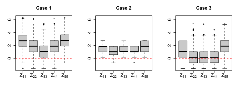
The first table of Table 1 shows the estimated power of the tests under different sample sizes. We see that the power of the tests increases as the sample size increases and the new tests outperform the existing tests in all cases. We further check the pattern of statistics under different cases (the second table of Table 1). We simulate 10,000 datasets when $n_{i}=10$ and there are 1,493 cases where all tests reject the null (Case 1), 15 cases where the only existing tests reject the null (FR, MCM, MCMM all reject; none of S, SS, A reject) (Case 2), and 558 cases where the only new tests reject the null (S, SS, A all reject; none of FR, MCM, MCMM reject) (Case 3) at 0.01 significance level.

We take a closer look at the test statistics and Figure 5 shows boxplots of within-sample statistics under each case, where $Z_{ii}=\left(R_{ii}-\textsf{E}(R_{ii})\right)/\sqrt{\textsf{Var}(R_{ii})}$ $(i=1,\ldots,5)$. Here, relatively large values of $Z_{ii}$ are the evidence against the null. In Case 3, $Z_{22}$, $Z_{33}$, and $Z_{44}$ are close to zero, which thus leads to poor performance of the existing tests. The new tests take into account both within-sample and between-sample statistics, and are more powerful. On the other hand, since the new tests are developed to cover a wide range of alternatives, the existing tests aimed at specific alternatives, e.g., location alternatives with small $K$ or symmetrically distributed alternatives, could show better performance. On other hand, even in Case 2, the new tests exhibit relatively small $p$-values as well (Table in Figure 5). More data analysis can be found in Appendix E.

In this paper, we propose new graph-based multi-sample tests for comparing multiple distributions by utilizing information embedded in groups as much as possible. When the number of samples or groups is large, computing pairwise distances for constructing the similarity graph could be computationally expensive. In this case, faster algorithms, such an approximate nearest neighbor algorithm that do not compute all pairwise distances [4], could be used to save time.

1. 1.

   For all authors…

   1. (a)

      Do the main claims made in the abstract and introduction accurately reflect the paper’s contributions and scope? [Yes]

   2. (b)

      Did you describe the limitations of your work? [Yes] See Section 5.

   3. (c)

      Did you discuss any potential negative societal impacts of your work? [No]

   4. (d)

      Have you read the ethics review guidelines and ensured that your paper conforms to them? [Yes]

2. 2.

   If you are including theoretical results…

   1. (a)

      Did you state the full set of assumptions of all theoretical results? [Yes] See Theorem 3.1 and Theorem 3.5.

   2. (b)

      Did you include complete proofs of all theoretical results? [Yes] See Appendix A and C.

3. 3.

   If you ran experiments…

   1. (a)

      Did you include the code, data, and instructions needed to reproduce the main experimental results (either in the supplemental material or as a URL)? [Yes] See the “code” folder in the supplementary material.

   2. (b)

      Did you specify all the training details (e.g., data splits, hyperparameters, how they were chosen)? [Yes] See Section 4.

   3. (c)

      Did you report error bars (e.g., with respect to the random seed after running experiments multiple times)? [No]

   4. (d)

      Did you include the total amount of compute and the type of resources used (e.g., type of GPUs, internal cluster, or cloud provider)? [No]

4. 4.

   If you are using existing assets (e.g., code, data, models) or curating/releasing new assets…

   1. (a)

      If your work uses existing assets, did you cite the creators? [Yes] See Section 5 for age image dataset.

   2. (b)

      Did you mention the license of the assets? [Yes] See Section 5.

   3. (c)

      Did you include any new assets either in the supplemental material or as a URL? [Yes] See Section 5 and “code” folder in the supplementary material.

   4. (d)

      Did you discuss whether and how consent was obtained from people whose data you’re using/curating? [Yes] See Section 5.

   5. (e)

      Did you discuss whether the data you are using/curating contains personally identifiable information or offensive content? [Yes] See Section 5.

5. 5.

   If you used crowdsourcing or conducted research with human subjects…

   1. (a)

      Did you include the full text of instructions given to participants and screenshots, if applicable? [N/A] We did not conduct research with human subjects.

   2. (b)

      Did you describe any potential participant risks, with links to Institutional Review Board (IRB) approvals, if applicable? [N/A]

   3. (c)

      Did you include the estimated hourly wage paid to participants and the total amount spent on participant compensation? [N/A]

References

- [1] Divyansh Agarwal, Somabha Mukherjee, Bhaswar Bikram Bhattacharya, and Nancy Ruonan Zhang. Distribution-free multisample test based on optimal matching with applications to single cell genomics. arXiv preprint arXiv:1906.04776, 2019.
- [2] Syed Mumtaz Ali and Samuel D Silvey. A general class of coefficients of divergence of one distribution from another. Journal of the Royal Statistical Society: Series B (Methodological), 28(1):131–142, 1966.
- [3] Yves Ismaël Ngounou Bakam and Denys Pommeret. K-sample test for equality of copulas. arXiv preprint arXiv:2112.05623, 2021.
- [4] Alina Beygelzimer, Sham Kakadet, John Langford, Sunil Arya, David Mount, and Shengqiao Li. Fnn: fast nearest neighbor search algorithms and applications. R package version, 1(1), 2013.
- [5] Song Cai, Jiahua Chen, and James V Zidek. Hypothesis testing in the presence of multiple samples under density ratio models. Statistica Sinica, pages 761–783, 2017.
- [6] Hao Chen, Xu Chen, and Yi Su. A weighted edge-count two-sample test for multivariate and object data. Journal of the American Statistical Association, (just-accepted), 2017.
- [7] Hao Chen and Jerome H Friedman. A new graph-based two-sample test for multivariate and object data. Journal of the American statistical association, 112(517):397–409, 2017.
- [8] Su Chen. A new distribution-free k-sample test: Analysis of kernel density functionals. Canadian Journal of Statistics, 48(2):167–186, 2020.
- [9] Alberto Ferrari. A note on sum and difference of correlated chi-squared variables. arXiv preprint arXiv:1906.09982, 2019.
- [10] Jerome H Friedman and Lawrence C Rafsky. Multivariate generalizations of the wald-wolfowitz and smirnov two-sample tests. The Annals of Statistics, pages 697–717, 1979.
- [11] Enrico Glaab, Anaïs Baudot, Natalio Krasnogor, Reinhard Schneider, and Alfonso Valencia. Enrichnet: network-based gene set enrichment analysis. Bioinformatics, 28(18):i451–i457, 2012.
- [12] Kyle L Grazier and William G’Sell. Group medical insurance claims database collection and analysis. Society of Actuaries, http://www. soa. org/files/pdf/Large_Claims_Report. pdf, 2004.
- [13] Norbert Henze. A multivariate two-sample test based on the number of nearest neighbor type coincidences. The Annals of Statistics, pages 772–783, 1988.
- [14] Norbert Henze and Mathew D Penrose. On the multivariate runs test. The Annals of Statistics, 27(1):290–298, 1999.
- [15] Ilmun Kim. Comparing a large number of multivariate distributions. arXiv preprint arXiv:1904.05741, 2019.
- [16] William H Kruskal et al. A nonparametric test for the several sample problem. The Annals of Mathematical Statistics, 23(4):525–540, 1952.
- [17] Ho Chung Leon Law, Dougal Sutherland, Dino Sejdinovic, and Seth Flaxman. Bayesian approaches to distribution regression. In International Conference on Artificial Intelligence and Statistics, pages 1167–1176, 2018.
- [18] Boris Yu Lemeshko and Irina V Veretelnikova. On some new k-samples tests for testing the homogeneity of distribution laws. In 2018 XIV International Scientific-Technical Conference on Actual Problems of Electronics Instrument Engineering (APEIE), pages 153–157. IEEE, 2018.
- [19] Weijun Luo, Michael S Friedman, Kerby Shedden, Kurt D Hankenson, and Peter J Woolf. Gage: generally applicable gene set enrichment for pathway analysis. BMC bioinformatics, 10(1):1–17, 2009.
- [20] S Mukhopadhyay and K Wang. Nonparametric high-dimensional k-sample comparison. Biometrika (to appear), 2020.
- [21] Dan Nettleton and T Banerjee. Testing the equality of distributions of random vectors with categorical components. Computational statistics & data analysis, 37(2):195–208, 2001.
- [22] Adam Petrie. Graph-theoretic multisample tests of equality in distribution for high dimensional data. Computational Statistics & Data Analysis, 96:145–158, 2016.
- [23] Maria L Rizzo, Gábor J Székely, et al. Disco analysis: A nonparametric extension of analysis of variance. The Annals of Applied Statistics, 4(2):1034–1055, 2010.
- [24] Paul R Rosenbaum. An exact distribution-free test comparing two multivariate distributions based on adjacency. Journal of the Royal Statistical Society: Series B (Statistical Methodology), 67(4):515–530, 2005.
- [25] Rasmus Rothe, Radu Timofte, and Luc Van Gool. Deep expectation of real and apparent age from a single image without facial landmarks. International Journal of Computer Vision, 126(2-4):144–157, 2018.
- [26] Mark F Schilling. Multivariate two-sample tests based on nearest neighbors. Journal of the American Statistical Association, 81(395):799–806, 1986.
- [27] Peng Shi, Xiaoping Feng, and Jean-Philippe Boucher. Multilevel modeling of insurance claims using copulas. The Annals of Applied Statistics, 10(2):834–863, 2016.
- [28] George PH Styan. Notes on the distribution of quadratic forms in singular normal variables. Biometrika, 57(3):567–572, 1970.
- [29] Jin Zhang and Yuehua Wu. k-sample tests based on the likelihood ratio. Computational Statistics & Data Analysis, 51(9):4682–4691, 2007.
- [30] Qingyang Zhang, Ghadeer Mahdi, Jian Tinker, and Hao Chen. A graph-based multi-sample test for identifying pathways associated with cancer progression. Computational Biology and Chemistry, 87:107285, 2020.