Efficient Adiabatic Rapid Passage in the Presence of Noise
Abstract
Adiabatic Rapid Passage (ARP) is a powerful technique for efficient transfer of population between quantum states. In the lab, the efficiency of ARP is often limited by noise on either the energies of the states or the frequency of the driving field. We study ARP in the simple setting of a two-level system subject to sinusoidal fluctuations on the energy level separation by numerically solving the optical Bloch equations in the absence of damping. We investigate the dependence of the efficiency of population transfer on the frequency and amplitude of the perturbation, and find that it is predominantly affected by resonant coupling when the detuning matches the frequency of the noise. We present intuitive principles for when ARP becomes inefficient within this model, and provide a sufficient condition for the population transfer to be above an arbitrary threshold.
I Introduction
Coherent population transfer is an important tool for state preparation in many systems, such as trapped ions Sørensen et al. 2006, Rydberg atoms Zhou et al. 2020; Beterov et al. 2016, molecules Dürr et al. 2004; Wang et al. 2015 and more. A common technique to achieve efficient population transfer in a two-level system is Adiabatic Rapid Passage (ARP), which typically sweeps the detuning of a driving field across resonance slowly in order to achieve full population transfer. Compared to other population inversion methods such as a -pulse (i.e. a resonant pulse with time-integrated area of ), an advantage of ARP is that it does not depend on precise control of the resonant frequency, or the amplitude and timing of the pulse. Therefore, ARP is robust against small changes in resonance, making it especially effective for population inversion in inhomogeneously broadened samples.
For ARP to be successful, the frequency sweep must be both “rapid” and “adiabatic”, as its name suggests. The sweep should be fast compared to the excited state lifetime, while slow compared to the period of a resonant Rabi oscillation. By the adiabatic theorem, if the sweep is sufficiently slow, then the quantum state of the system adiabatically follows the instantaneous energy eigenstate Kato 1950. Far from resonance, the bare states and those dressed by the driving field coincide, while at resonance an avoided-crossing occurs. The lower eigenstate is adiabatically connected to the ground state when detuning , and is connected to the excited state when . Therefore, when an atom starts in the ground state and the field detuning slowly changes from to (where ), the atom remains in the lower eigenstate, becoming excited by the end of the chirp, thus achieving population inversion. In the case where detuning is chirped linearly in time, the efficiency of population transfer by ARP is given by the Landau-Zener formula Wittig 2005, and depends on the speed of the sweep.
In practice, ARP is performed in finite time, over a finite frequency range, and is subject to noise from the environment. Therefore, studying the performance of ARP in these realistic scenarios is crucial to testing its robustness. There have been many studies on the effect of both “off-diagonal noise,” which is related to fluctuations of the coupling strength between levels, and “diagonal noise,” which is related to fluctuations of the separation between energy levels. Off-diagonal coloured Gaussian noise has been studied in Pokrovsky and Sinitsyn 2002; Kenmoe et al. 2013, slow off-diagonal noise in Luo and Raikh 2017, and off-diagonal harmonic noise in Kraft et al. 2013. Here, we investigate the effect of diagonal noise, which has been studied in the large amplitude and rapid fluctuation limit with a stochastic model in Kayanuma 1984a; Kayanuma 1984b. We aim to understand the effect of perturbations with arbitrary profiles, by focusing on the sinusoidal time-variation of the energy level separation due to a single Fourier component of the noise. The setup of the problem and the system Hamiltonian will be presented in Section II. The results of our simulations and their implications will be discussed in Section III. In particular, we investigate the role of resonances between the noise and the system, and study how the effect depends on the frequency and amplitude of the noise. We also present a comparison between our simulations and a non-adiabatic model presented in Chasseur et al. 2015 that noticed similar behavior. Finally, we end with a discussion on noise tolerance, and find a condition for good population transfer despite the noise.
II The Two-Level System and Hamiltonian
We consider a two-level system driven by an external field with linearly chirped frequency. The energy difference between the levels is subject to a sinusoidal perturbation, which represents the noise on the system. An energy level diagram is shown in Figure 1,
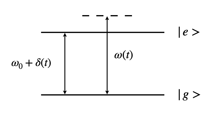
where is the unperturbed energy difference between the two levels, and is the perturbation, given by . The frequency of the driving field is chirped linearly across resonance so that . The detuning between the driving field and the system is therefore .
Under the Rotating-Wave Approximation (RWA), the Hamiltonian of the system can be written as
| (1) |
where , are the ground and excited states and is the bare Rabi frequency. For simplicity, we set in the following discussions.
Figure 2 shows the instantaneous eigenvalues of the Hamiltonian in three different regimes. In the limit of small-amplitude noise (i.e. , Fig 2(a)), the noise is a weak perturbation on the Landau-Zener Hamiltonian, , and one would expect the effect of the noise on the population transfer to be very weak. In the limit of small noise frequency (i.e. duration of the sweep, Figure 2(b)), the noise appears almost linear during the sweep time, , so that the detuning as a function of time can be viewed simply as a new linear sweep with slope and shifted endpoints. When is much less than the duration of the sweep and the amplitude of the noise is moderate, as shown in Figure 2(c), the effect of the noise can no longer be explained by the simple intuitions for the previous two limiting cases. This regime is the focus of discussion in the following section.


III Discussion
III.1 Noise resonances
Without the noise term , the Hamiltonian becomes
| (2) |
Under the assumption that , , the problem has a well-known analytic solution: the fraction of atoms that undergo a diabatic transition is given by the Landau-Zener formula Zener 1932
| (3) |
which means the fraction of atoms that end up in the exited state is . In the limit of slow sweeps (), all atoms adiabatically follow the dressed state and end up in the excited state. An example of a noiseless ARP sweep over a finite frequency range ( to ) is presented in Figure 3(a), which shows the trajectory of the Bloch vector on the Bloch sphere, and the excited state population over time. The atomic population that starts in the ground state makes a transition as detuning sweeps across zero, and ends up in the excited state by the end of the process.


With a sinusoidal perturbation , the evolution becomes more complicated primarily because additional resonances occur when reaches an integer multiple of the noise frequency Ashhab et al. 2007, as exemplified in Figure 3(b). The occurrence of these additional resonances can be understood as the result of frequency modulation on the driving field. The frequency modulation leads to sidebands with frequencies () away from the carrier frequency. The sidebands resonate with the system during the sweep when the aforementioned condition is reached, giving rise to additional “noise resonances.” Such noise resonances are problematic in an ARP process, because they can compromise the efficiency of population transfer. As the detuning sweeps across these noise resonances, unwanted population transfer occurs, resulting in a suboptimal excited state population at the end of the process. This becomes clear in the example shown in Figure 3(b). In a noisy ARP sweep, beside the population transfer near zero detuning, there are two other population jumps (which show up on the Bloch sphere as spirals) that occur when the resonance condition with the noise is reached. As a consequence, the final transfer efficiency is well below the ideal result.
To confirm that the noise affects population transfer primarily by means of noise resonances, rather than some other interaction with the system, we present another example in Figure 3(c), which shows an ARP sweep under the same noise as the previous example, but with a shortened sweep range, so that the noise frequency falls outside the range of detuning chirp, which means the noise resonance condition is never reached. The noise in this case causes the Bloch vector trajectory to oscillate about the adiabatic trajectory in Figure 3(a), but without significant deviations. Accordingly, the transfer efficiency of the sweep is comparable to that of the noiseless case.
III.2 Noise parameters and ARP efficiency
While it seems like the efficiency loss associated with the noise can be circumvented by simply shortening the range of the sweep, this is not always possible since the noise in an experiment might have multiple frequency components or even a continuous frequency spectrum. It is therefore worthwhile to investigate the relation between population transfer efficiency of the ARP sweep, , and parameters of the noise, namely its frequency , amplitude , and phase . We note that while population transfer can have a phase dependence, the goal of our investigation is to understand the effect of noise, where the phase is unknown and varies from shot to shot. Therefore in the following discussion, the results we present are always phase-averaged.
Figure 4 shows the efficiency of noisy ARP sweeps with a fixed noise amplitude and variable frequency. Note that the efficiency goes to unity as the noise frequency approaches zero, which corresponds to the limiting case of Fig. 2(b). The efficiency also goes to 1 as the noise frequency exceeds the range of the sweep (), as discussed in the previous section. In between these two limits, population transfer depends critically on the noise frequency: in this example, a noise with frequency leads to almost zero transfer, whereas a noise with frequency results in a transfer efficiency of 1. oscillates as a function of in this regime. The oscillation becomes faster as increases and is modulated by an envelope which goes to 1 in the limits of both small and large . The spacing between adjacent peaks of the oscillating function depends inversely on .

Figure 5(a) plots as a function of both and . The graph has a striped pattern, where the spacing between adjacent stripes is consistent with our previous observation, i.e. proportional to . This spacing also depends inversely on the sweep rate, as shown in Figure 5(b) and 5(c). Note that Figure 5(b) and 5(c) only shows a small range of noise frequency around . Many other notable features of Figure 5, such as the tilting of the stripes, and the vanishing of the strip patterns at large amplitudes, will be further explored in the following section in comparison to a simplified model.


III.3 Comparison with the “multi-jump” model
The same Hamiltonian is studied in Chasseur et al. 2015, but in the diabatic regime (), and in the context of optimal control. A simplified model (the “multi-jump” model) for the state’s evolution is proposed, which focuses on what happens when the detuning crosses a noise resonance. Every sweep across a resonance is modeled by multiplying the state vector with a unitary matrix. By construction, this model simulates only the population jumps at resonances , and disregards the small oscillations that occur in between.
By comparing predictions of the multi-jump model with our simulations, we find that it is a good predictor of the final population transfer in the fast-sweep regime, which is the regime for which the model is intended. But even outside its native regime, the model performs surprisingly well in capturing some important features of the population transfer efficiency .
Figure 6 compares the ARP efficiencies predicted by our simulations and by the multi-jump model. The simplified model makes two important predictions: a horizontal striped pattern that becomes less distinct when ; and regions of maximum population transfer when (). These conditions are marked in Figure 6(a) and 6(b), which display the prediction by the model and the result of our simulations. While does not predict the correct maxima in the simulations, it gives the correct vertical spacing between adjacent strips, which, as we observed in the previous section, is inversely related to and positively related to sweep rate . The multi-jump model fails to predict the tilting and distortion of the striped pattern, and we have yet to find an intuitive explanation for this observation.
The maximum transfer condition predicted by the multi-jump model is equivalent to requiring that the noise be in phase at all noise resonances (i.e. when , where ). At the point in the ARP sweep when sidebands of the frequency-modulated driving field become resonant with the system, if they all have the same phase, then they contribute constructively to the population transfer (Fig. 7(a)); if the phase at adjacent noise resonances is out of phase, then they contribute destructively (Fig. 7(b)).
The critical ratio is marked in Figure 6. This is roughly the boundary of the striped pattern, and comes from the first zero of the Bessel function . According to Chasseur et al. 2015, this is the condition for the bare resonance () to be suppressed by the population transfer at the noise resonances.


III.4 Noise tolerance
From a practical perspective, it is useful to quantify the level of noise an ARP sweep can tolerate, while still having a reasonably high population transfer efficiency. Since the standard for high efficiency can differ between applications, we proceed by considering an arbitrary threshold between 0 and 1. We define any ARP sweep with efficiency to be “acceptable,” where is the ideal efficiency given by the Landau-Zener formula, .
One way to quantify noise tolerance is to determine, for a given frequency of noise, the maximum amplitude the noise can have such that the efficiency of the sweep is still acceptable. This characterization is done in Figure 8(a), which shows the maximum acceptable amplitude for a range of noise frequencies, with a sweep rate of and threshold of . We observe that while the maximum allowable noise amplitude varies considerably with small changes in , a sufficient lower boundary exists and depends linearly on . Below this sufficient condition (the orange line in Figure 8(a)), the population transfer is guaranteed to be above the threshold value (in this example, 99%).


Figure 8(b) demonstrates that the slope of this sufficient boundary depends on the sweep rate of the ARP, where the acceptable threshold is set to . Here, we notice that the slope() appears linear (on a logarithmic scale), up to . The same is true for results by the multi-jump model, which are plotted in red.
Based on the multi-jump model, keeping only the contribution of -1st, 0th, and 1st order resonances (which is a good approximation when the noise is not too strong, because the higher order sidebands due to frequency modulation are negligible when modulation amplitude is small), we find an explicit expression for the excited state fraction , which depends on and . From here we obtain a lower bound for , assuming and , given by
| (4) |
Then a sufficient condition for is , which leads to
| (5) |
and thus
| (6) |
Eq. 6 provides a sufficient condition for an ARP efficiency to be above the threshold . As shown in Figure 8(b), up to , Eq. 6 agrees excellently with the multi-jump points, and is close to the simulation points. The discrepancy is due to the fact that the model is used outside of its intended regime (the diabatic limit).
IV Conclusion
By performing numerical simulations, we find that, in the presence of sinusoidal noise, the efficiency of ARP is influenced by resonances that occur between the system and the noise. The noise has less of an effect, in general, if the amplitude is small, or if its frequency is low or high. Specifically, if the noise frequency exceeds the full range over which the detuning is chirped, then its effect on population transfer is almost negligible. The ARP efficiency depends critically on noise frequency in the intermediate frequency regime. The regions in parameter space with maximum transfer efficiency are similar to those predicted by the diabatic multi-jump model. While the functional form of the efficiency is complicated, we propose a sufficient condition to achieve high population transfer by studying the worst-case scenario, which can be used to quantify noise tolerance in an ARP process.
V Acknowledgements
The authors would like to thank Joseph McGowan and Nick Mantella for helpful discussions, as well as Dr. Yuval Sanders for kindly answering our questions about his paper Chasseur et al. 2015. This work was supported by the Natural Sciences and Engineering Research Council of Canada. AMS is a Fellow of CIFAR.
References
- Sørensen et al. (2006) J. L. Sørensen, D. Møller, T. Iversen, J. B. Thomsen, F. Jensen, P. Staanum, D. Voigt, and M. Drewsen, 8, 261 (2006).
- Zhou et al. (2020) M.-T. Zhou, J.-L. Liu, P.-F. Sun, Z.-Y. An, J. Li, X.-H. Bao, and J.-W. Pan, Phys. Rev. A 102, 013706 (2020).
- Beterov et al. (2016) I. I. Beterov, M. Saffman, E. A. Yakshina, D. B. Tretyakov, V. M. Entin, S. Bergamini, E. A. Kuznetsova, and I. I. Ryabtsev, Phys. Rev. A 94, 062307 (2016).
- Dürr et al. (2004) S. Dürr, T. Volz, A. Marte, and G. Rempe, Phys. Rev. Lett. 92, 020406 (2004).
- Wang et al. (2015) F. Wang, X. He, X. Li, B. Zhu, J. Chen, and D. Wang, 17, 035003 (2015).
- Kato (1950) T. Kato, Journal of the Physical Society of Japan 5, 435 (1950), https://doi.org/10.1143/JPSJ.5.435 .
- Wittig (2005) C. Wittig, The Journal of Physical Chemistry B 109, 8428 (2005).
- Pokrovsky and Sinitsyn (2002) V. L. Pokrovsky and N. A. Sinitsyn, (2002), 10.1103/PhysRevB.67.144303.
- Kenmoe et al. (2013) M. B. Kenmoe, H. N. Phien, M. N. Kiselev, and L. C. Fai, Physical review. B, Condensed matter and materials physics 87 (2013), 10.1103/PhysRevB.87.224301.
- Luo and Raikh (2017) Z.-X. Luo and M. E. Raikh, Physical review. B 95 (2017), 10.1103/PhysRevB.95.064305.
- Kraft et al. (2013) M. Kraft, S. Burkhardt, R. Mannella, and S. Wimberger, Fluctuation and Noise Letters 12, 1340005 (2013).
- Kayanuma (1984a) Y. Kayanuma, Journal of the Physical Society of Japan 53, 108 (1984a), https://doi.org/10.1143/JPSJ.53.108 .
- Kayanuma (1984b) Y. Kayanuma, Journal of the Physical Society of Japan 53, 118 (1984b), https://doi.org/10.1143/JPSJ.53.118 .
- Chasseur et al. (2015) T. Chasseur, L. S. Theis, Y. R. Sanders, D. J. Egger, and F. K. Wilhelm, Phys. Rev. A 91, 043421 (2015).
- Zener (1932) C. Zener, Proceedings of the Royal Society of London. Series A, Containing papers of a mathematical and physical character 137, 696 (1932).
- Ashhab et al. (2007) S. Ashhab, J. R. Johansson, A. M. Zagoskin, and F. Nori, Phys. Rev. A 75, 063414 (2007).
- Malinovsky and Krause (2001) V. Malinovsky and J. Krause, The European Physical Journal D - Atomic, Molecular, Optical and Plasma Physics 14 (2001), 10.1007/s100530170212.
- Noel et al. (2012) T. Noel, M. R. Dietrich, N. Kurz, G. Shu, J. Wright, and B. B. Blinov, Phys. Rev. A 85, 023401 (2012).
*