跳到论文正文
W Papers独立论文阅读器 arXiv:2205.13684 论文正文 计算阅读时间 · 0%
引用这篇论文根据当前论文元数据生成,正式投稿前建议核对。


License: arXiv.org perpetual non-exclusive license
arXiv:2205.13684v2 [stat.ML] 09 Nov 2022

Learning with Stochastic Orders

Carles Domingo-Enrich Affiliation: Courant Institute of Mathematical Sciences, New York University    Yair Schiff Affiliation: IBM Research AI    Youssef Mroueh Affiliation: IBM Research AI
Abstract

Learning high-dimensional distributions is often done with explicit likelihood modeling or implicit modeling via minimizing integral probability metrics (IPMs). In this paper, we expand this learning paradigm to stochastic orders, namely, the convex or Choquet order between probability measures. Towards this end, exploiting the relation between convex orders and optimal transport, we introduce the Choquet-Toland distance between probability measures, that can be used as a drop-in replacement for IPMs. We also introduce the Variational Dominance Criterion (VDC) to learn probability measures with dominance constraints, that encode the desired stochastic order between the learned measure and a known baseline. We analyze both quantities and show that they suffer from the curse of dimensionality and propose surrogates via input convex maxout networks (ICMNs), that enjoy parametric rates. We provide a min-max framework for learning with stochastic orders and validate it experimentally on synthetic and high-dimensional image generation, with promising results. Finally, our ICMNs class of convex functions and its derived Rademacher Complexity are of independent interest beyond their application in convex orders.

1 Introduction

Learning complex high-dimensional distributions with implicit generative models [Goodfellow et al. 2014, Mohamed and Lakshminarayanan 2017, Arjovsky et al. 2017] via minimizing integral probability metrics (IPMs) [Müller 1997a] has lead to the state of the art generation across many data modalities [Karras et al. 2019, De Cao and Kipf 2018, Padhi et al. 2020]. An IPM compares probability distributions with a witness function belonging to a function class ℱ\mathcal{F}, e.g., the class of Lipchitz functions, which makes the IPM correspond to the Wasserstein distance 1. While estimating the witness function in such large function classes suffer from the curse of dimensionality, restricting it to a class of neural networks leads to the so called neural net distance [Arora et al. 2017] that enjoys statistical parametric rates.

In probability theory, the question of comparing distributions is not limited to assessing only equality between two distributions. Stochastic orders were introduced to capture the notion of dominance between measures. Similar to IPMs, stochastic orders can be defined by looking at the integrals of measures over function classes ℱ\mathcal{F} [Müller 1997b]. Namely, for μ+,μ−∈𝒫1​(ℝd)\mu_{+},\mu_{-}\in\mathcal{P}_{1}(\mathbb{R}^{d}), μ+\mu_{+} dominates μ−\mu_{-}, or μ−⪯μ+\mu_{-}\preceq\mu_{+}, if for any function f∈ℱf\in\mathcal{F}, we have ∫ℝdf⁡(x)​d​μ−​(x)≤∫ℝdf⁡(x)​d​μ+​(x)\int_{\mathbb{R}^{d}}f(x)\,d\mu_{-}(x)\leq\int_{\mathbb{R}^{d}}f(x)\,d\mu_{+}(x) (See 1(a) for an example). In the present work, we focus on the Choquet or convex order [Ekeland and Schachermayer 2014] generated by the space of convex functions (See Sec. 2 for more details).

Previous work has focused on learning with stochastic orders in the one dimensional setting, as it has prominent applications in mathematical finance and distributional reinforcement learning (RL). The survival function gives a characterisation of the convex order in one dimension (See 1(b) and Sec. 2 for more details). For instance, in portfolio optimization [Xue et al. 2020, Post et al. 2018, Dentcheva and Ruszczynski 2003] the goal is to find the portfolio that maximizes a utility under dominance constraints of a known benchmark or baseline. A similar concept was introduced in distributional RL [Martin et al. 2020] for learning policies with dominance constraints on the distribution of the reward. While these works are limited to the univariate setting, our work is the first, to the best of our knowledge, that provides a computationally tractable characterization of stochastic orders that is scalable in high dimensions and is sample efficient.

The paper is organized as follows: we introduce in Sec. 3 the Variational Dominance Criterion (VDC); the VDC between measures μ+\mu_{+} and μ−\mu_{-} takes value 0 if and only if μ+\mu_{+} dominates μ−\mu_{-} in the convex order. The VDC suffers from the curse of dimension and can not be estimated efficiently from samples. To remediate this, we introduce in Sec. 4, a VDC surrogate via Input Convex Maxout Networks (ICMNs). ICMNs are new variants of Input Convex Neural Nets Amos et al. 2017 that we propose as proxy for convex functions and study their complexity. We show in Sec. 4 that the surrogate VDC has parametric rates and can be efficiently estimated from samples. The surrogate VDC can be computed using (stochastic) gradient descent on the parameters of the ICMN and can characterize convex dominance (See 1(c)). We then show in Sec. 5 how to use the VDC and its surrogate to define a pseudo distance on the probability Space. Finally we propose in Sec. 6 penalizing generative models training losses with the surrogate VDC to learn implicit generative models that have better coverage and spread than known baselines. This leads to a min-max game similar to GANs. We validate our framework in Sec. 7 with experiments on portfolio optimization and image generation.

Refer to caption
(a)
Refer to caption
(b)
Refer to caption
(c)
Figure 1: VDC example in 1D. 1(a) :μ+\mu_{+} is mixture of 3 Gaussians , μ−\mu_{-} corresponds to a single mode of the mixture. μ+\mu_{+} dominates μ−\mu_{-} in the convex order. 1(b) : uni-variate characterization of the convex order with survival functions (See Sec. 2 for details). 1(c): Surrogate VDC computation with Input Convex Maxout Network and gradient descent. The surrogate VDC tends to zero at the end of the training and hence characterizes the convex dominance of μ+\mu_{+} on μ−\mu_{-}.

2 The Choquet or convex order

Denote by 𝒫⁡(ℝd)\mathcal{P}(\mathbb{R}^{d}) the set of Borel probability measures on ℝd\mathbb{R}^{d} and by 𝒫1​(ℝd)⊂𝒫⁡(ℝd)\mathcal{P}_{1}(\mathbb{R}^{d})\subset\mathcal{P}(\mathbb{R}^{d}) the subset of those which have finite first moment: μ∈𝒫1​(ℝ)\mu\in\mathcal{P}_{1}(\mathbb{R}) if and only if ∫ℝd‖x‖​𝑑μ​(x)<+∞\int_{\mathbb{R}^{d}}\|x\|\,d\mu(x)<+\infty.

Comparing probability distributions

Integral probability metrics (IPMs) are pseudo-distances between probability measures μ,ν\mu,\nu defined as dℱ​(μ,ν)=supf∈ℱ𝔼μ​f−𝔼ν​fd_{\mathcal{F}}(\mu,\nu)=\sup_{f\in\mathcal{F}}\mathbb{E}_{\mu}f-\mathbb{E}_{\nu}f, for a given function class ℱ\mathcal{F} which is symmetric with respect to sign flips. They are ubiquitous in optimal transport and generative modeling to compare distributions: if ℱ\mathcal{F} is the set of functions with Lipschitz constant 1, then the resulting IPM is the 1-Wasserstein distance; if ℱ\mathcal{F} is the unit ball of an RKHS, the IPM is its maximum mean discrepancy. Clearly, dℱ​(μ,ν)=0d_{\mathcal{F}}(\mu,\nu)=0 if and only 𝔼μ​f=𝔼ν​f\mathbb{E}_{\mu}f=\mathbb{E}_{\nu}f for all f∈ℱf\in\mathcal{F}, and when ℱ\mathcal{F} is large enough, this is equivalent to μ=ν\mu=\nu.

The Choquet or convex order

When the class ℱ\mathcal{F} is not symmetric with respect to sign flips, comparing the expectations 𝔼μ​f\mathbb{E}_{\mu}f and 𝔼ν​f\mathbb{E}_{\nu}f for f∈ℱf\in\mathcal{F} does not yield a pseudo-distance. In the case where ℱ\mathcal{F} is the set of convex functions, the convex order naturally arises instead:

Definition 1 (Choquet order, Ekeland and Schachermayer 2014, Def. 4).

For μ−,μ+∈𝒫1​(ℝd)\mu_{-},\mu_{+}\in\mathcal{P}_{1}(\mathbb{R}^{d}), we say that μ−⪯μ+\mu_{-}\preceq\mu_{+} if for any convex function f:ℝd→ℝf:\mathbb{R}^{d}\to\mathbb{R}, we have

∫ℝdf⁡(x)​d​μ−​(x)≤∫ℝdf⁡(x)​d​μ+​(x).\textstyle\int_{\mathbb{R}^{d}}f(x)\,d\mu_{-}(x)\leq\int_{\mathbb{R}^{d}}f(x)\,d\mu_{+}(x). (1)

μ−⪯μ+\mu_{-}\preceq\mu_{+} is classically denoted as “μ−\mu_{-} is a balayée of μ+\mu_{+}", or “μ+\mu_{+} dominates μ−\mu_{-}". It turns out that ⪯\preceq is a partial order on 𝒫1​(ℝd)\mathcal{P}_{1}(\mathbb{R}^{d}), meaning that reflexivity (μ⪯μ\mu\preceq\mu), antisymmetry (if μ⪯ν\mu\preceq\nu and ν⪯μ\nu\preceq\mu, then μ=ν\mu=\nu), and transitivity (if μ1⪯μ2\mu_{1}\preceq\mu_{2} and μ2⪯μ3\mu_{2}\preceq\mu_{3}, then μ1⪯μ3\mu_{1}\preceq\mu_{3}) hold. As an example, if μ−\mu_{-}, μ+\mu_{+} are Gaussians μ−=N⁡(0,Σ−)\mu_{-}=N(0,\Sigma_{-}), μ+=N⁡(0,Σ+)\mu_{+}=N(0,\Sigma_{+}), then μ−⪯μ+\mu_{-}\preceq\mu_{+} if and only if Σ−⪯Σ+\Sigma_{-}\preceq\Sigma_{+} in the positive-semidefinite order [Müller 2001]. Also, since linear functions are convex, μ−⪯μ+\mu_{-}\preceq\mu_{+} implies that both measures have the same expectation: 𝔼x∼μ−​x=𝔼x∼μ+​x\mathbb{E}_{x\sim\mu_{-}}x=\mathbb{E}_{x\sim\mu_{+}}x.

In the univariate case, μ−⪯μ+\mu_{-}\preceq\mu_{+} implies that supp⁡(μ−)⊆supp⁡(μ+)\mathrm{supp}(\mu_{-})\subseteq\mathrm{supp}(\mu_{+}) and that Var⁡(μ−)≤Var⁡(μ+)\mathrm{Var}(\mu_{-})\leq\mathrm{Var}(\mu_{+}), and we have that μ−⪯μ+\mu_{-}\preceq\mu_{+} holds if and only if for all x∈ℝx\in\mathbb{R}, ∫x+∞F¯μ−​(t)​𝑑t≤∫x+∞F¯μ+​(t)​𝑑t\int_{x}^{+\infty}\bar{F}_{\mu_{-}}(t)\,dt\leq\int_{x}^{+\infty}\bar{F}_{\mu_{+}}(t)\,dt, where F¯⋅\bar{F}_{\cdot} is the survival function (one minus the cumulative distribution function). Note that this characterization can be checked efficiently if one has access to samples of μ−\mu_{-} and μ+\mu_{+}.

In the high-dimensional case, there exists an alternative characterization of the convex order:

Proposition 1 (Ekeland and Schachermayer 2014, Thm. 10).

If μ−,μ+∈𝒫1​(ℝd)\mu_{-},\mu_{+}\in\mathcal{P}_{1}(\mathbb{R}^{d}), we have μ−⪯μ+\mu_{-}\preceq\mu_{+} if and only if there exists a Markov kernel RR (i.e. ∀x∈ℝd\forall x\in\mathbb{R}^{d}, ∫ℝdy​d​Rx​(y)=x\int_{\mathbb{R}^{d}}y\,dR_{x}(y)=x) such that μ+=∫ℝdRx​d​μ−\mu_{+}=\int_{\mathbb{R}^{d}}R_{x}\,d\mu_{-}.

Equivalently, there exists a coupling (X,Y)(X,Y) such that Law⁡(X)=μ−\mathrm{Law}(X)=\mu_{-}, Law⁡(Y)=μ+\mathrm{Law}(Y)=\mu_{+} and X=𝔼⁡(Y|X)X=\mathbb{E}(Y|X) almost surely. Intuitively, this means that μ+\mu_{+} is more spread out than μ−\mu_{-}. Remark that this characterization is difficult to check, especially in high dimensions.

3 The Variational Dominance Criterion

In this section, we present a quantitative way to deal with convex orders. Given a bounded open convex subset Ω⊆ℝd\Omega\subseteq\mathbb{R}^{d} and a compact set 𝒦⊆ℝd\mathcal{K}\subseteq\mathbb{R}^{d}, let 𝒜={u:Ω→ℝ,u convex and ∇u∈𝒦 almost everywhere}\mathcal{A}=\{u:\Omega\to\mathbb{R},\ u\text{ convex and }\nabla u\in\mathcal{K}\text{ almost everywhere}\}. We define the Variational Dominance Criterion (VDC) between probability measures μ+\mu_{+} and μ−\mu_{-} supported on Ω\Omega in analogously to IPMs, replacing ℱ\mathcal{F} by 𝒜\mathcal{A}:

VDC𝒜(μ+||μ−):=supu∈𝒜∫Ωud(μ−−μ+).\textstyle\mathrm{VDC}_{\mathcal{A}}(\mu_{+}||\mu_{-}):=\sup_{u\in\mathcal{A}}\int_{\Omega}u\,d(\mu_{-}-\mu_{+}). (2)

Remark that when 0∈𝒦0\in\mathcal{K}, VDC𝒜(μ+||μ−)≥0\mathrm{VDC}_{\mathcal{A}}(\mu_{+}||\mu_{-})\geq 0 because the zero function belongs to the set 𝒜\mathcal{A}. We reemphasize that since 𝒜\mathcal{A} is not symmetric with respect to sign flips as f∈𝒜f\in\mathcal{A} does not imply −f∈𝒜-f\in\mathcal{A}, the properties of the VDC are very different from those of IPMs. Most importantly, the following proposition, shown in App. A, links the VDC to the Choquet order.

Proposition 2.

Let 𝒦\mathcal{K} compact such that the origin belongs to the interior of 𝒦\mathcal{K}. If μ+,μ−∈𝒫⁡(Ω)\mu_{+},\mu_{-}\in\mathcal{P}(\Omega), VDC𝒜(μ+||μ−):=supu∈𝒜∫Ωud(μ−−μ+)=0\mathrm{VDC}_{\mathcal{A}}(\mu_{+}||\mu_{-}):=\sup_{u\in\mathcal{A}}\int_{\Omega}u\,d(\mu_{-}-\mu_{+})=0 if and only if ∫Ωu​d​(μ−−μ+)≤0\int_{\Omega}u\,d(\mu_{-}-\mu_{+})\leq 0 for any convex function on Ω\Omega (i.e. μ−⪯μ+\mu_{-}\preceq\mu_{+} according to the Choquet order).

That is, Prop. 2 states that the VDC between μ+\mu_{+} and μ−\mu_{-} takes value 0 if and only if μ+\mu_{+} dominates μ−\mu_{-}. Combining this with the interpretation of Prop. 1, we see that intuitively, the quantity VDC𝒜(μ+||μ−)\mathrm{VDC}_{\mathcal{A}}(\mu_{+}||\mu_{-}) is small when μ+\mu_{+} is more spread out than μ−\mu_{-}, and large otherwise. Hence, if we want to enforce or induce a Choquet ordering between two measures in an optimization problem, we can include the VDC (or rather, its surrogate introduced in Sec. 4) as a penalization term in the objective. Before this, we explore the connections between VDC and optimal transport, and study some statistical properties of the VDC.

3.1 The VDC and optimal transport

Toland duality provides a way to interpret the VDC through the lens of optimal transport. In the following, W2​(μ,ν)W_{2}(\mu,\nu) denotes the 2-Wasserstein distance between μ\mu and ν\nu.

Theorem 1 (Toland duality, adapted from Thm. 1 of Carlier 2008).

For any μ+,μ−∈𝒫⁡(Ω)\mu_{+},\mu_{-}\in\mathcal{P}(\Omega), the VDC satisfies:

VDC𝒜(μ+||μ−)=supν∈𝒫⁡(𝒦){12W22(μ+,ν)−12W22(μ−,ν)}−12∫Ω∥x∥2d(μ+−μ−)(x)\displaystyle\mathrm{VDC}_{\mathcal{A}}(\mu_{+}||\mu_{-})=\sup_{\nu\in\mathcal{P}(\mathcal{K})}\left\{\frac{1}{2}W_{2}^{2}(\mu_{+},\nu)-\frac{1}{2}W_{2}^{2}(\mu_{-},\nu)\right\}-\frac{1}{2}\int_{\Omega}\|x\|^{2}\ d(\mu_{+}-\mu_{-})(x) (3)

The optimal convex function uu of VDC in (2) and the optimal ν\nu in the right-hand side of (3) satisfy (∇u)#​μ+=(∇u)#​μ−=ν(\nabla{u})_{\#}\mu_{+}=(\nabla{u})_{\#}\mu_{-}=\nu, where (∇u)#​μ+(\nabla{u})_{\#}\mu_{+} denotes the pushforward of μ+\mu_{+} by ∇u\nabla{u}.

Note that under the assumption 0∈𝒦0\in\mathcal{K}, Thm. 1 implies that VDC𝒜(μ+||μ−)=0\mathrm{VDC}_{\mathcal{A}}(\mu_{+}||\mu_{-})=0 if and only if W22​(μ+,ν)−12​∫Ω‖x‖2​d​μ+≤W22​(μ−,ν)−12​∫Ω‖x‖2​d​μ−W_{2}^{2}(\mu_{+},\nu)-\frac{1}{2}\int_{\Omega}\|x\|^{2}\ d\mu_{+}\leq W_{2}^{2}(\mu_{-},\nu)-\frac{1}{2}\int_{\Omega}\|x\|^{2}\ d\mu_{-} for any ν∈𝒫⁡(𝒦)\nu\in\mathcal{P}(\mathcal{K}). Under the equivalence VDC𝒜(μ+||μ−)=0⇔μ+⪰μ−\mathrm{VDC}_{\mathcal{A}}(\mu_{+}||\mu_{-})=0\iff\mu_{+}\succeq\mu_{-} shown by Prop. 2, this provides yet another characterization of the convex order for arbitrary dimension.

3.2 Statistical rates for VDC estimation

In this subsection, we prove an upper bound on the statistical rate of estimation of VDC𝒜(μ||ν)\mathrm{VDC}_{\mathcal{A}}(\mu||\nu) using the estimator VDC𝒜(μn||νn)\mathrm{VDC}_{\mathcal{A}}(\mu_{n}||\nu_{n}) based on the empirical distributions μn=1n​∑i=1nδxi\mu_{n}=\frac{1}{n}\sum_{i=1}^{n}\delta_{x_{i}}, νn=1n​∑i=1nδyi\nu_{n}=\frac{1}{n}\sum_{i=1}^{n}\delta_{y_{i}} built from i.i.d. samples (xi)i=1n(x_{i})_{i=1}^{n}, (yi)i=1n(y_{i})_{i=1}^{n} from μ\mu and ν\nu, respectively.

Theorem 2.

Let Ω=[−1,1]d\Omega=[-1,1]^{d} and 𝒦={x∈ℝd|‖x‖2≤C}\mathcal{K}=\{x\in\mathbb{R}^{d}\,|\,\|x\|_{2}\leq C\} for an arbitrary C>0C>0. With probability at least 1−δ1-\delta,

|VDC𝒜(μ||ν)−VDC𝒜(μn||νn)|≤18​C2​d​log⁡(δ4)(2n)+8Kn−2d,\textstyle|\mathrm{VDC}_{\mathcal{A}}(\mu||\nu)-\mathrm{VDC}_{\mathcal{A}}(\mu_{n}||\nu_{n})|\leq\sqrt{18C^{2}d\log(\frac{\delta}{4})}(\frac{2}{\sqrt{n}})+8Kn^{-\frac{2}{d}}, (4)

where 𝒦\mathcal{K} depends on CC and dd.

The dependency on n−2dn^{-\frac{2}{d}} is indicative of the curse of dimension: we need a number of samples nn exponential in dd to control the estimation error. While Thm. 2 only shows an upper bound on the difference between the VDC and its estimator, in Subsec. 5.1 we study a related setting where a Ω~​(n−2d)\tilde{\Omega}(n^{-\frac{2}{d}}) lower bound is available. Hence, we hypothesize that VDC estimation is in fact cursed by dimension in general.

4 A VDC surrogate via input convex maxout networks

Given the link between the VDC and the convex order, one is inclined to use the VDC as a quantitative proxy to induce convex order domination in optimization problems. Estimating the VDC implies solving an optimization problem over convex functions. In practice, we only have access to the empirical versions μn,νn\mu_{n},\nu_{n} of the probability measures μ,ν\mu,\nu; we could compute the VDC between the empirical measures by solving a linear program similar to the ones used in non-parametric convex regression [Hildreth 1954]. However, the statistical rates for the VDC estimation from samples are cursed by dimension (Subsec. 3.2), which means that we would need a number of samples exponential in the dimension to get a good estimate. Our approach is to focus on a surrogate problem instead:

supu∈𝒜^∫Ωu​d​(μ−−μ+),\textstyle\sup_{u\in\hat{\mathcal{A}}}\,\int_{\Omega}u\ d(\mu_{-}-\mu_{+}), (5)

where 𝒜^\hat{\mathcal{A}} is a class of neural network functions included in 𝒜\mathcal{A} over which we can optimize efficiently. In constructing 𝒜^\hat{\mathcal{A}}, we want to hardcode the constraints uu convex and ∇u∈𝒦\nabla u\in\mathcal{K} almost everywhere into the neural network architectures. A possible approach would be to use the input convex neural networks (ICNNs) introduced by Amos et al. 2017, which have been used as a surrogate of convex functions for generative modeling with normalizing flows [Huang et al. 2021] in optimal transport Korotin et al. 2021a, Korotin et al. 2021b, Huang et al. 2021, Makkuva et al. 2020 and large scale Wasserstein flows Alvarez-Melis et al. 2021, Bunne et al. 2021, Mokrov et al. 2021.

However, we found in early experimentation that a superior alternative is to use input convex maxout networks (ICMNs), which are maxout networks [Goodfellow et al. 2013] that are convex with respect to inputs. Maxout networks and ICMNs are defined as follows:

Definition 2 (Maxout networks).

For a depth L≥2L\geq 2, let ℳ=(m1,…,mL)\mathcal{M}=(m_{1},\dots,m_{L}) be a vector of positive integers such that m1=dm_{1}=d. Let FL,ℳ,kF_{L,\mathcal{M},k} be the space of kk-maxout networks of depth LL and widths ℳ\mathcal{M}, which contains functions of the form

f⁡(x)=1mL​∑i=1mLai​maxj∈[k]​⟨wi,j(L−1),(x(L−1),1)⟩,ai∈ℝ,wi,j(L−1)∈ℝmL−1+1\textstyle f(x)=\frac{1}{\sqrt{m_{L}}}\sum_{i=1}^{m_{L}}a_{i}\max_{j\in[k]}\langle w^{(L-1)}_{i,j},(x^{(L-1)},1)\rangle,\qquad a_{i}\in\mathbb{R},\,w^{(L-1)}_{i,j}\in\mathbb{R}^{m_{L-1}+1} (6)

where for any 2≤ℓ≤L−12\leq\ell\leq L-1, and any 1≤i≤mℓ1\leq i\leq m_{\ell}, the ii-th component of x(ℓ)=(x1(ℓ),…,xmℓ(ℓ))x^{(\ell)}=(x^{(\ell)}_{1},\dots,x^{(\ell)}_{m_{\ell}}) is computed recursively as:

xi(ℓ)=1mℓ​maxj∈[k]​⟨wi,j(ℓ−1),(x(ℓ−1),1)⟩,wi,j(ℓ)∈ℝmℓ+1,\textstyle x^{(\ell)}_{i}=\frac{1}{\sqrt{m_{\ell}}}\max_{j\in[k]}\langle w^{(\ell-1)}_{i,j},(x^{(\ell-1)},1)\rangle,\qquad w^{(\ell)}_{i,j}\in\mathbb{R}^{m_{\ell}+1}, (7)

with x(1)=xx^{(1)}=x.

Definition 3 (Input convex maxout networks or ICMNs).

A maxout network ff of the form (6)-(7) is an input convex maxout network if (i) for any 1≤i≤ML1\leq i\leq M_{L}, ai≥0a_{i}\geq 0, and (ii) for any 2<ℓ≤L−12<\ell\leq L-1, 1≤i≤mℓ+11\leq i\leq m_{\ell+1}, 1≤j≤k1\leq j\leq k, the first mℓm_{\ell} components of wi,j(ℓ)w^{(\ell)}_{i,j} are non-negative. We denote the space of ICMNs as FL,ℳ,k,+F_{L,\mathcal{M},k,+}.

In other words, a maxout network is an ICMN if all the non-bias weights beyond the first layer are constrained to be non-negative. This definition is analogous to the one of ICNNs in Amos et al. 2017, which are also defined as neural networks with positivity constraints on non-bias weights beyond the first layer. Prop. 5 in App. B shows that ICMNs are convex w.r.t to their inputs.

It remains to impose the condition ∇u∈𝒦\nabla u\in\mathcal{K} almost everywhere, which in practice is enforced by adding the norms of the weights as a regularization term to the loss function. For theoretical purposes, we define FL,ℳ,k​(1)F_{L,\mathcal{M},k}(1) (resp. FL,ℳ,k,+​(1)F_{L,\mathcal{M},k,+}(1)) as the subset of FL,ℳ,kF_{L,\mathcal{M},k} (resp. FL,ℳ,k,+F_{L,\mathcal{M},k,+}) such that for all 1≤ℓ≤L−11\leq\ell\leq L-1, 1≤i≤mℓ1\leq i\leq m_{\ell}, 1≤j≤k1\leq j\leq k, ‖wi,j(ℓ)‖2≤1\|w^{(\ell)}_{i,j}\|_{2}\leq 1, and ‖a‖2=∑i=1mLai2≤1\|a\|_{2}=\sum_{i=1}^{m_{L}}a_{i}^{2}\leq 1. The following proposition, proven in App. B, shows simple bounds on the values of the functions in FL,ℳ,k​(1)F_{L,\mathcal{M},k}(1) and their derivatives.

Proposition 3.

Let ff be an ICMN that belongs to FL,ℳ,k​(1)F_{L,\mathcal{M},k}(1). For xx almost everywhere in ℬ1​(ℝd)\mathcal{B}_{1}(\mathbb{R}^{d}), ‖∇f​(x)‖≤1\|\nabla f(x)\|\leq 1. Moreover, for all x∈ℬ1​(ℝd)x\in\mathcal{B}_{1}(\mathbb{R}^{d}), |f⁡(x)|≤L|f(x)|\leq L, and for 1≤ℓ≤L1\leq\ell\leq L, ‖x(ℓ)‖≤ℓ\|x^{(\ell)}\|\leq\ell.

When 𝒦=ℬ1​(ℝd)\mathcal{K}=\mathcal{B}_{1}(\mathbb{R}^{d}), we have that the space of ICMNs FL,ℳ,k,+​(1)F_{L,\mathcal{M},k,+}(1) is included in 𝒜\mathcal{A}. Hence, we define the surrogate VDC associated to FL,ℳ,k,+​(1)F_{L,\mathcal{M},k,+}(1) as:

VDCFL,ℳ,k,+​(1)(μ+||μ−)=supu∈FL,ℳ,k,+​(1)∫Ωu​d​(μ−−μ+).\textstyle\begin{split}\textstyle\mathrm{VDC}_{F_{L,\mathcal{M},k,+}(1)}(\mu_{+}||\mu_{-})&\textstyle=\sup_{u\in F_{L,\mathcal{M},k,+}(1)}\int_{\Omega}u\,d(\mu_{-}-\mu_{+}).\end{split} (8)
Theorem 3.

Suppose that for all 1≤ℓ≤L1\leq\ell\leq L, the widths mℓm_{\ell} satisfy mℓ≤mm_{\ell}\leq m, and assume that μ,ν\mu,\nu are supported on the ball of ℝd\mathbb{R}^{d} of radius rr. With probability at least 1−δ1-\delta,

|VDCFL,ℳ,k,+​(1)(μ||ν)−VDCFL,ℳ,k,+​(1)(μn||νn)|\textstyle|\mathrm{VDC}_{F_{L,\mathcal{M},k,+}(1)}(\mu||\nu)-\mathrm{VDC}_{F_{L,\mathcal{M},k,+}(1)}(\mu_{n}||\nu_{n})| (9)
≤18​r2​log⁡(δ4)​(2n)+512​(L−1)​k​m​(m+1)n​((L+1)​log⁡(2)+log⁡(L2+1)2+π2),\textstyle\leq\sqrt{18r^{2}\log(\frac{\delta}{4})}\big(\frac{2}{\sqrt{n}}\big)+512\sqrt{\frac{(L-1)km(m+1)}{n}}\big(\sqrt{(L+1)\log(2)+\frac{\log(L^{2}+1)}{2}}+\frac{\sqrt{\pi}}{2}\big), (10)

We see from Thm. 3 that VDCFL,ℳ,k,+​(1)\mathrm{VDC}_{F_{L,\mathcal{M},k,+}(1)} in contrast to VDC𝒜\mathrm{VDC}_{\mathcal{A}} has parametric rates and hence favorable properties to be estimated from samples. In the following section, wes see that VDC can be used to defined a pseudo-distance on the probability space.

5 From the convex order back to a pseudo-distance

We define the Choquet-Toland distance (CT distance) as the map dCT,𝒜:𝒫⁡(Ω)×𝒫⁡(Ω)→ℝd_{\text{CT},\mathcal{A}}:\mathcal{P}(\Omega)\times\mathcal{P}(\Omega)\to\mathbb{R} given by

dCT,𝒜(μ+,μ−):=VDC𝒜(μ+||μ−)+VDC𝒜(μ−||μ+).\textstyle d_{\text{CT},\mathcal{A}}(\mu_{+},\mu_{-}):=\mathrm{VDC}_{\mathcal{A}}(\mu_{+}||\mu_{-})+\mathrm{VDC}_{\mathcal{A}}(\mu_{-}||\mu_{+}). (11)

That is, the CT distance between μ+\mu_{+} and μ−\mu_{-} is simply the sum of Variational Dominance Criteria. Applying Thm. 1, we obtain that dCT,𝒜​(μ+,μ−)=12​(supν∈𝒫⁡(𝒦){W22​(μ+,ν)−W22​(μ−,ν)}+supν∈𝒫⁡(𝒦){W22​(μ+,ν)−W22​(μ−,ν)})d_{\text{CT},\mathcal{A}}(\mu_{+},\mu_{-})=\frac{1}{2}(\sup_{\nu\in\mathcal{P}(\mathcal{K})}\left\{W_{2}^{2}(\mu_{+},\nu)-W_{2}^{2}(\mu_{-},\nu)\right\}+\sup_{\nu\in\mathcal{P}(\mathcal{K})}\left\{W_{2}^{2}(\mu_{+},\nu)-W_{2}^{2}(\mu_{-},\nu)\right\}). The following result, shown in App. C, states that dC​T,Kd_{CT,K} is indeed a distance.

Theorem 4.

Suppose that the origin belongs to the interior of 𝒦\mathcal{K}. dCT,𝒜d_{\text{CT},\mathcal{A}} is a distance, i.e. it fulfills

  1. (i)

    dCT,𝒜​(μ+,μ−)≥0d_{\text{CT},\mathcal{A}}(\mu_{+},\mu_{-})\geq 0 for any μ+,μ−∈𝒫⁡(Ω)\mu_{+},\mu_{-}\in\mathcal{P}(\Omega) (non-negativity).

  2. (ii)

    dCT,𝒜​(μ+,μ−)=0d_{\text{CT},\mathcal{A}}(\mu_{+},\mu_{-})=0 if and only if μ+=μ−\mu_{+}=\mu_{-} (identity of indiscernibles).

  3. (iii)

    If μ1,μ2,μ3∈𝒫⁡(Ω)\mu_{1},\mu_{2},\mu_{3}\in\mathcal{P}(\Omega), we have that dCT,𝒜​(μ1,μ2)≤dCT,𝒜​(μ1,μ3)+dCT,𝒜​(μ3,μ2)d_{\text{CT},\mathcal{A}}(\mu_{1},\mu_{2})\leq d_{\text{CT},\mathcal{A}}(\mu_{1},\mu_{3})+d_{\text{CT},\mathcal{A}}(\mu_{3},\mu_{2}).

As in (8), we define the surrogate CT distance as:

dCT,FL,ℳ,k,+​(1)​(μ+,μ−)\textstyle d_{\text{CT},F_{L,\mathcal{M},k,+}(1)}(\mu_{+},\mu_{-}) =VDCFL,ℳ,k,+​(1)(μ+||μ−)+VDCFL,ℳ,k,+​(1)(μ−||μ+).\textstyle=\mathrm{VDC}_{F_{L,\mathcal{M},k,+}(1)}(\mu_{+}||\mu_{-})+\mathrm{VDC}_{F_{L,\mathcal{M},k,+}(1)}(\mu_{-}||\mu_{+}). (12)

5.1 Statistical rates for CT distance estimation

We show almost-tight upper and lower bounds on the expectation of the Choquet-Toland distance between a probability measure and its empirical version. Namely, 𝔼⁡[dCT,𝒜​(μ,μn)]=O⁡(n−2d),Ω⁡(n−2d/log⁡(n))\mathbb{E}[d_{\text{CT},\mathcal{A}}(\mu,\mu_{n})]=O(n^{-\frac{2}{d}}),\Omega(n^{-\frac{2}{d}}/\log(n)).

Theorem 5.

Let C0,C1C_{0},C_{1} be universal constants independent of the dimension dd. Let Ω=[−1,1]d\Omega=[-1,1]^{d}, and 𝒦={x∈ℝd|‖x‖2≤C}\mathcal{K}=\{x\in\mathbb{R}^{d}\,|\,\|x\|_{2}\leq C\}. Let μn\mu_{n} be the nn-sample empirical measure corresponding to a probability measure μ\mu over [−1,1]d[-1,1]^{d}. When μ\mu is the uniform probability measure and n≥C1​log⁡(d)n\geq C_{1}\log(d), we have that

𝔼⁡[dCT,𝒜​(μ,μn)]≥C0​Cd⁡(1+C)​log⁡(n)​n−2d.\textstyle\mathbb{E}[d_{\text{CT},\mathcal{A}}(\mu,\mu_{n})]\geq C_{0}\sqrt{\frac{C}{d(1+C)\log(n)}}n^{-\frac{2}{d}}. (13)

For any probability measure μ\mu over [−1,1]d[-1,1]^{d},

𝔼⁡[dCT,𝒜​(μ,μn)]≤K​n−2d,\textstyle\mathbb{E}[d_{\text{CT},\mathcal{A}}(\mu,\mu_{n})]\leq Kn^{-\frac{2}{d}}, (14)

where KK is a constant depending on CC and dd (but not the measure μ\mu).

Overlooking logarithmic factors, we can summarize Thm. 5 as 𝔼⁡[dCT,𝒜​(μ,μn)]≍n−2d\mathbb{E}[d_{\text{CT},\mathcal{A}}(\mu,\mu_{n})]\asymp n^{-\frac{2}{d}}. The estimation of the CT distance is cursed by dimension: one needs a sample size exponential with the dimension dd for μn\mu_{n} to be at a desired distance from μ\mu. It is also interesting to contrast the rate n−2dn^{-\frac{2}{d}} with the rates for similar distances. For example, for the rr-Wasserstein distance we have 𝔼⁡[Wrr​(μ,μn)]≍n−rd\mathbb{E}[W_{r}^{r}(\mu,\mu_{n})]\asymp n^{-\frac{r}{d}} (Singh and Póczos 2018, Section 4). Given the link of the CT distance and VDC with the squared 2-Wasserstein distance (see Subsec. 3.1), the n−2dn^{-\frac{2}{d}} rate is natural.

The proof of Thm. 5, which can be found in App. D, is based on upper-bounding and lower-bounding the metric entropy of the class of bounded Lipschitz convex functions with respect to an appropriate pseudo-norm. Then we use Dudley’s integral bound and Sudakov minoration to upper and lower-bound the Rademacher complexity of this class, and we finally show upper and lower bounds of the CT distance by the Rademacher complexity. Bounds on the metric entropy of bounded Lipschitz convex functions have been computed and used before [Balazs et al. 2015, Guntuboyina and Sen 2013], but in LpL^{p} and supremum norms, not in our pseudo-norm.

Next, we see that the surrogate CT distance defined in (12) does enjoy parametric estimation rates.

Theorem 6.

Suppose that for all 1≤ℓ≤L1\leq\ell\leq L, the widths mℓm_{\ell} satisfy mℓ≤mm_{\ell}\leq m. We have that

𝔼⁡[dCT,FL,ℳ,k,+​(1)​(μ,μn)]\textstyle\mathbb{E}[d_{\text{CT},F_{L,\mathcal{M},k,+}(1)}(\mu,\mu_{n})] ≤256​(L−1)​k​m​(m+1)n​((L+1)​log⁡(2)+log⁡(L2+1)2+π2),\textstyle\leq 256\sqrt{\frac{(L-1)km(m+1)}{n}}\left(\sqrt{(L+1)\log(2)+\frac{\log(L^{2}+1)}{2}}+\frac{\sqrt{\pi}}{2}\right), (15)

In short, we have that 𝔼⁡[dCT,FL,ℳ,k,+​(1)​(μ,μn)]=O⁡(L​m​kn)\mathbb{E}[d_{\text{CT},F_{L,\mathcal{M},k,+}(1)}(\mu,\mu_{n})]=O(Lm\sqrt{\frac{k}{n}}). Hence, if we take the number of samples nn larger than kk times the squared product of width and depth, we can make the surrogate CT distance small. Thm. 6, proven in App. D, is based on a Rademacher complexity bound for the space FL,ℳ,k​(1)F_{L,\mathcal{M},k}(1) of maxout networks which may be of independent interest; to our knowledge, existing Rademacher complexity bounds for maxout networks are restricted to depth-two networks [Balazs et al. 2015, Kontorovich 2018].

Theorems 5 and 6 show the advantages of the surrogate CT distance over the CT distance are not only computational but also statistical; the CT distance is such a strong metric that moderate-size empirical versions of a distribution are always very far from it. Hence, it is not a good criterion to compare how close an empirical distribution is to a population distribution. In contrast, the surrogate CT distance between a distribution and its empirical version is small for samples of moderate size. An analogous observation for the Wasserstein distance versus the neural net distance was made by Arora et al. 2017.

If μn\mu_{n}, νn\nu_{n} are empirical versions of μ,ν\mu,\nu, it is also interesting to bound |dCT,FL,ℳ,k,+​(1)​(μn,νn)−dCT,𝒜​(μ,ν)|≤|dCT,FL,ℳ,k,+​(1)​(μn,νn)−dCT,FL,ℳ,k,+​(1)​(μ,ν)|+|dCT,FL,ℳ,k,+​(1)​(μ,ν)−dCT,𝒜​(μ,ν)||d_{\text{CT},F_{L,\mathcal{M},k,+}(1)}(\mu_{n},\nu_{n})-d_{\text{CT},\mathcal{A}}(\mu,\nu)|\leq|d_{\text{CT},F_{L,\mathcal{M},k,+}(1)}(\mu_{n},\nu_{n})-d_{\text{CT},F_{L,\mathcal{M},k,+}(1)}(\mu,\nu)|+|d_{\text{CT},F_{L,\mathcal{M},k,+}(1)}(\mu,\nu)-d_{\text{CT},\mathcal{A}}(\mu,\nu)|. The first term has a O⁡(k/n)O(\sqrt{k/n}) bound following from Thm. 6, while the second term is upper-bounded by 2​supf∈𝒜inff~∈FL,ℳ,k​(1)‖f−f~‖∞2\sup_{f\in\mathcal{A}}\inf_{\tilde{f}\in F_{L,\mathcal{M},k}(1)}\|f-\tilde{f}\|_{\infty}, which is (twice) the approximation error of the class 𝒜\mathcal{A} by the class FL,ℳ,k​(1)F_{L,\mathcal{M},k}(1). Such bounds have only been derived in L=2L=2: Balazs et al. 2015 shows that supf∈𝒜inff~∈F2,(d,1),k​(1)∥f−f~∥∞=O(dk−2/d)\sup_{f\in\mathcal{A}}\inf_{\tilde{f}\in F_{2,(d,1),k}(1)}\|f-\tilde{f}\|_{\infty}=O(dk^{-2/d}). Hence, we need kk exponential in dd to make the second term small, and thus n≫kn\gg k exponential in dd to make the first term small.

6 Learning distributions with the surrogate VDC and CT distance

We provide a min-max framework to learn distributions with stochastic orders. As in the generative adversarial network (GAN, Goodfellow et al. 2014, Arjovsky et al. 2017) framework, we parametrize probability measures implicitly as the pushforward μ=g#​μ0\mu=g_{\#}\mu_{0} of a base measure μ0\mu_{0} by a generator function gg in a parametric class 𝒢\mathcal{G} and we optimize over gg. The loss functions involve a maximization over ICMNs corresponding to the computation of a surrogate VDC or CT distance (and possibly additional maximization problems), yielding a min-max problem analogous to GANs.

Enforcing dominance constraints with the surrogate VDC. In some applications, we want to optimize a loss L:𝒫⁡(Ω)→ℝL:\mathcal{P}(\Omega)\to\mathbb{R} under the constraint that μ=g#​μ0\mu=g_{\#}\mu_{0} dominates a baseline measure ν\nu. We can enforce, or at least, bias μ\mu towards the dominance constraint by adding a penalization term proportional to the surrogate VDC between μ\mu and ν\nu, in application of Prop. 2.

A first instance of this approach appears in portfolio optimization [Xue et al. 2020, Post et al. 2018]. Let ξ=(ξ1,…,ξp)\xi=(\xi_{1},\dots,\xi_{p}) be a random vector of return rates of pp assets and let Y1:=G1​(ξ)Y_{1}:=G_{1}(\xi), Y2:=G2​(ξ)Y_{2}:=G_{2}(\xi) be real-valued functions of ξ\xi which represent the return rates of two different asset allocations or portfolios, e.g. Gi​(ξ)=⟨ωi,ξ⟩G_{i}(\xi)=\langle\omega_{i},\xi\rangle with ωi∈ℝp\omega_{i}\in\mathbb{R}^{p}. The goal is to find a portfolio G2G_{2} that enhances a benchmark portfolio G1G_{1} in a certain way. For a portfolio GG with return rate Y:=G⁡(ξ)Y:=G(\xi), we let FY(1)​(x)=Pξ​(Y≤x)F_{Y}^{(1)}(x)=P_{\xi}(Y\leq x) be the CDF of its return rate, and FY(2)​(x)=∫−∞xFY(1)​(x′)​d​x′F_{Y}^{(2)}(x)=\int_{-\infty}^{x}F_{Y}^{(1)}(x^{\prime})\,dx^{\prime}. If Y1,Y2Y_{1},Y_{2} are the return rates of G1,G2G_{1},G_{2}, we say that Y2Y_{2} dominates Y1Y_{1} in second order, or Y2⪰2Y1Y_{2}\succeq_{2}Y_{1} if for all x∈ℝx\in\mathbb{R}, FY2(2)​(x)≤FY1(2)​(x)F_{Y_{2}}^{(2)}(x)\leq F_{Y_{1}}^{(2)}(x), which intuitively means that the return rates Y2Y_{2} are less spread out than those Y1Y_{1}, i.e. the risk is smaller. Formally, the portfolio optimization problem can be written as:

maxG2𝔼[Y2:=G2(ξ)],s.t.Y2⪰2Y1:=G1(ξ).\textstyle\max_{G_{2}}\ \mathbb{E}[Y_{2}:=G_{2}(\xi)],\qquad\mathrm{s.t.}\ Y_{2}\succeq_{2}Y_{1}:=G_{1}(\xi). (16)

It turns out that Y2⪰2Y1Y_{2}\succeq_{2}Y_{1} if and only if 𝔼⁡[(η−Y2)+]≤𝔼⁡[(η−Y1)+]\mathbb{E}[(\eta-Y_{2})_{+}]\leq\mathbb{E}[(\eta-Y_{1})_{+}] for any η∈ℝ\eta\in\mathbb{R}, or yet equivalently, if 𝔼⁡[u⁡(Y2)]≥𝔼⁡[u⁡(Y1)]\mathbb{E}[u(Y_{2})]\geq\mathbb{E}[u(Y_{1})] for all concave non-decreasing u:ℝ→ℝu:\mathbb{R}\to\mathbb{R} [Dentcheva and Ruszczyński 2004]. Although different, note that the second order is intimately connected to the Choquet order for 1-dimensional distributions, and it can be handled with similar tools. Define FL,ℳ,k,−+(1)F_{L,\mathcal{M},k,-+}(1) as the subset of FL,ℳ,k,+​(1)F_{L,\mathcal{M},k,+}(1) such that the first m1m_{1} components of the weights wi,j(1)w^{(1)}_{i,j} are non-positive for all 1≤i≤m21\leq i\leq m_{2}, 1≤j≤k1\leq j\leq k. If we set the input width m1=1m_{1}=1, we can encode the condition Y2⪰2Y1Y_{2}\succeq_{2}Y_{1} as VDCFL,ℳ,k,−+(1)(ν||μ)\mathrm{VDC}_{F_{L,\mathcal{M},k,-+}(1)}(\nu||\mu), where ν=ℒ⁡(Y1)\nu=\mathcal{L}(Y_{1}) and μ=ℒ⁡(Y2)\mu=\mathcal{L}(Y_{2}) are the distributions of Y1Y_{1}, Y2Y_{2}, resp. Hence, with the appropriate Lagrange multiplier we convert problem (16) into a min-max problem between μ\mu and the potential uu of VDC\mathrm{VDC}

minμ:μ=ℒ⁡(⟨ξ,ω2⟩)−∫ℝxdμ(x)+λVDCFL,ℳ,k,−+(1)(ν||μ).\textstyle\min_{\mu:\mu=\mathcal{L}(\langle\xi,\omega_{2}\rangle)}\ -\int_{\mathbb{R}}x\,d\mu(x)+\lambda\mathrm{VDC}_{F_{L,\mathcal{M},k,-+}(1)}(\nu||\mu). (17)

A second instance of this approach is in GAN training. Assuming that we have a baseline generator g0g_{0} that can be obtained via regular training, we consider the problem:

ming∈𝒢{maxf∈ℱ{𝔼X∼νn[f(X)]−𝔼Y∼μ0[f(g(Y))]}+λVDCFL,ℳ,k,+​(1)(g#μ0||(g0)#μ0)}.\textstyle\min_{g\in\mathcal{G}}\left\{\max_{f\in\mathcal{F}}\{\mathbb{E}_{X\sim\nu_{n}}[f(X)]-\mathbb{E}_{Y\sim\mu_{0}}[f(g(Y))]\}+\lambda\mathrm{VDC}_{F_{L,\mathcal{M},k,+}(1)}(g_{\#}\mu_{0}||(g_{0})_{\#}\mu_{0})\right\}. (18)

The first term in the objective function is the usual WGAN loss [Arjovsky et al. 2017], although it can be replaced by any other standard GAN loss. The second term, which is proportional to VDCFL,ℳ,k,+​(1)(g#μ0||(g0)#μ0)=maxu∈FL,ℳ,k,+​(1){𝔼Y∼μ0[u(g0(Y))]−𝔼Y∼μ0[u(g(Y))]}\mathrm{VDC}_{F_{L,\mathcal{M},k,+}(1)}(g_{\#}\mu_{0}||(g_{0})_{\#}\mu_{0})=\max_{u\in F_{L,\mathcal{M},k,+}(1)}\{\mathbb{E}_{Y\sim\mu_{0}}[u(g_{0}(Y))]-\mathbb{E}_{Y\sim\mu_{0}}[u(g(Y))]\}, enforces that g#​μ0⪰(g0)#​μ0g_{\#}\mu_{0}\succeq(g_{0})_{\#}\mu_{0} in the Choquet order, and thus uu acts as a second ‘Choquet’ critic. Tuning λ\lambda appropriately, the rationale is that we want a generator that optimizes the standard GAN loss, with the condition that the generated distribution dominates the baseline distribution. As stated by Prop. 1, dominance in the Choquet order translates to g#​μ0g_{\#}\mu_{0} being more spread out than (g0)#​μ0(g_{0})_{\#}\mu_{0}, which should help avoid mode collapse and improve the diversity of generated samples. In practice, this min-max game is solved via Algorithm 1 given in App. F. For the Choquet critic, this amounts to an SGD step followed by a projection step to impose non-negativity of hidden to hidden weights.

Generative modeling with the surrogate CT distance.

The surrogate Choquet-Toland distance is well-suited for generative modeling, as it can used in GANs in place of the usual discriminator. Namely, if ν\nu is a target distribution, νn\nu_{n} is its empirical distribution, and 𝒟={μ=g#​μ0|g∈𝒢}\mathcal{D}=\{\mu=g_{\#}\mu_{0}|g\in\mathcal{G}\} is a class of distributions that can be realized as the push-forward of a base measure μ0∈𝒫⁡(ℝd0)\mu_{0}\in\mathcal{P}(\mathbb{R}^{d_{0}}) by a function g:ℝd0→ℝdg:\mathbb{R}^{d_{0}}\to\mathbb{R}^{d}, the problem to solve is g∗=argming∈𝒢dCT,FL,ℳ,k,+​(1)​(g#​μ0,νn)=argming∈𝒢{maxu∈FL,ℳ,k,+​(1)⁡{𝔼X∼νn​[u⁡(X)]−𝔼Y∼μ0​[u⁡(g⁡(Y))]}+maxu∈FL,ℳ,k,+​(1)⁡{𝔼Y∼μ0​[u⁡(g⁡(Y))]−𝔼X∼νn​[u⁡(X)]}}g^{*}=\argmin_{g\in\mathcal{G}}d_{\text{CT},F_{L,\mathcal{M},k,+}(1)}(g_{\#}\mu_{0},\nu_{n})=\argmin_{g\in\mathcal{G}}\{\max_{u\in F_{L,\mathcal{M},k,+}(1)}\{\mathbb{E}_{X\sim\nu_{n}}[u(X)]-\mathbb{E}_{Y\sim\mu_{0}}[u(g(Y))]\}+\max_{u\in F_{L,\mathcal{M},k,+}(1)}\{\mathbb{E}_{Y\sim\mu_{0}}[u(g(Y))]-\mathbb{E}_{X\sim\nu_{n}}[u(X)]\}\}. Algorithm 2 given in App. F summarizes learning with the surrogate CT distance.

7 Experiments

Portfolio optimization under dominance constraints

In this experiment, we use the VDC to optimize an illustrative example from Xue et al. 2020 (Example 1) that follows the paradigm laid out in Sec. 6. In this example, ξ∈ℝ∼P\xi\in\mathbb{R}\sim P is drawn uniformly from [0,1][0,1], we define the benchmark portfolio as:

G1​(ξ)={i20ξ∈[0.05×i,0.05×(i+1))i=0,…,191ξ=1G_{1}(\xi)=\begin{cases}\frac{i}{20}&\xi\in[0.05\times i,0.05\times(i+1))\ \ \ \ i=0,\ldots,19\\ 1&\xi=1\end{cases}

and the optimization is over the parameterized portfolio G2​(ξ):=G⁡(ξ,z)=z​ξG_{2}(\xi):=G(\xi;z)=z\xi.

The constrained optimization problem is thus specified as:

minz−𝔼P[G(ξ;z)]s.t.G(ξ;z)⪰2G1(ξ), 1≤z≤2\min_{z}\ \ -\mathbb{E}_{P}[G(\xi;z)]\ \ \ \mathrm{s.t.}\ \ G(\xi;z)\succeq_{2}G_{1}(\xi),\ 1\leq z\leq 2

As stated in Xue et al. 2020, this example has a known solution at z=2z=2 where 𝔼P​[G2​(ξ,2)]=1\mathbb{E}_{P}[G_{2}(\xi;2)]=1 outperforms the benchmark 𝔼P​[G1​(ξ)]=0.5.\mathbb{E}_{P}[G_{1}(\xi)]=0.5. We relax the constrained optimization by including it in the objective function, thus creating min-max game (17) introduced in Sec. 6. We parameterize FL,ℳ,k,−+(1)F_{L,\mathcal{M},k,-+}(1) with a 3-layer, fully-connected, decreasing ICMN with hidden dimension 32 and maxout kernel size of 4. After 5000 steps of stochastic gradient descent on zz (learning rate 1e−3\mathrm{e}^{-3}) and the parameters of the ICMN (learning rate 1e−3\mathrm{e}^{-3}), using a batch size of 512 and λ=1\lambda=1, we are able to attain accurate approximate values of the known solution: z=2,z=2, 1512​∑j=1512[Gz​(ξj)]=1.042,\frac{1}{512}\sum_{j=1}^{512}[G_{z}(\xi_{j})]=1.042, and 1512​∑j=1512[G1​(ξj)]=0.496.\frac{1}{512}\sum_{j=1}^{512}[G_{1}(\xi_{j})]=0.496.

Refer to caption
(a) g∗g^{*} CIFAR-10 samples
Refer to caption
Refer to caption
Refer to caption
(b) Initialisation
Refer to caption
Refer to caption
Refer to caption
(c) 5k iterations
Refer to caption
Refer to caption
Refer to caption
(d) 80k iterations
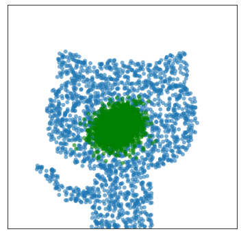
Figure 2: Training generative models by enforcing dominance with surrogate VDC on pre-trained CIFAR-10 WGAN-GP (Left) and with surrogate CT distance on 2D point clouds (Right). Ground truth point cloud distributions (blue) consist of swiss roll (Top), circle of eight gaussians (Middle), and Github icon converted to a point cloud (Bottom).

Image generation with baseline model dominance

Another application of learning with the VDC is in the high-dimensional setting of CIFAR-10 [Krizhevsky and Hinton 2009] image generation. As detailed in Sec. 6, we start by training a baseline generator g0g_{0} using the regularized Wasserstein-GAN paradigm (WGAN-GP) introduced in Arjovsky et al. 2017, Gulrajani et al. 2017, where gradient regularization is computed for the discriminator with respect to interpolates between real and generated data. When training g∗g^{*} and g0g_{0}, we used the same WGAN-GP hyperparameter configuration. We set λ\lambda in Equation (18) to 10 (see App. F and App. H for more details).

Table 1: FID scores for WGAN-GP and WGAN-GP with VDC surrogate for convex functions approximated by either ICNNs with softplus activations or ICMNs. ICMNs improve upon the baseline g0g_{0} and outperform ICNNs with softplus. FID score for WGAN-GP + VDC includes mean values ±\pm one standard deviation for 5 repeated runs with different random initialization seeds.
FID
g0g_{0}: WGAN-GP 69.67
g∗g^{*}: WGAN-GP + VDC CP-Flow ICNN 83.470 ±\pm 3.732
g∗g^{*}: WGAN-GP + VDC ICMN (Ours) 67.317 ±\pm 0.776

Training runs for g∗g^{*} and g0g_{0} were performed in computational environments that contained 1 CPU and 1 A100 GPU. To evaluate performance of g∗g^{*} vs. g0g_{0}, we rely on the Fréchet Inception Distance (FID) introduced in Heusel et al. 2017. Note that when training a WGAN-GP baseline from scratch we used hyperparameters that potentially differ from those used in state-of-the-art implementations. Additionally, for computing FIDs we use a pytorch-lightning implementation of the inception network, which is different from the widely used Tensorflow implementation [Salimans et al. 2016], resulting in potential discrepancies in our reported baseline FID and those in the literature. FID results are reported in Table 1, where we see improved image quality from g∗g^{*} (as measured by lower FID) relative to the pre-trained baseline g0g_{0}. We therefore find that the VDC surrogate improves upon g0g_{0} by providing g∗g^{*} with larger support, preventing mode collapse. Samples generated from g∗g^{*} are displayed in 2(a).

In order to highlight the representation power of ICMNs, we replace them in the VDC estimation by the ICNN implementation of Huang et al. 2021. Instead of maxout activation, Huang et al. 2021 uses a Softplus activation and instead of a projection step it also uses a Softplus operation to impose the non-negativity of hidden to hidden weights to enforce convexity. We see in Table 1 that VDC’s estimation with ICMN outperforms Huang et al. 2021 ICNNs. While ICMNs have maximum of affine functions as a building block, ICNN’s proof of universality in Huang et al. 2021 relies on approximating the latter, this could be one of the reason behind ICMN superiority.

Probing mode collapse To investigate how training with the surrogate VDC regularizer helps alleviate mode collapse in GAN training, we implemented GANs trained with the IPM objective alone and compared this to training with the surrogate VDC regularizer for a mixture of 8 Gaussians target distribution. In Figure 3 given in App. G we quantify mode collapse by looking at two scores: 1) the entropy of the discrete assignment of generated points to the means of the mixture 2) the negative log likelihood (NLL) of the Gaussian mixture. When training with the VDC regularizer to improve upon the collapsed generator g0g_{0} (which is taken from step 55k from the unregularized GAN training), we see more stable training and better mode coverage as quantified by our scores.

2D point cloud generation with dC​Td_{CT} We apply learning with the CT distance in a 2D generative modeling setting. Both the generator and CT critic architectures are comprised of fully-connected neural networks with maxout non-linearities of kernel size 2. Progression of the generated samples can be found in the right-hand panel of Figure 2, where we see the trained generator accurately learn the ground truth distribution. All experiments were performed in a single-CPU compute environment.

8 Conclusion

In this paper, we introduced learning with stochastic order in high dimensions via surrogate Variational Dominance Criterion and Choquet-Toland distance. These surrogates leverage input convex maxout networks, a new variant of input convex neural networks. Our surrogates have parametric statistical rates and lead to new learning paradigms by incorporating dominance constraints that improve upon a baseline. Experiments on synthetic and real image generation yield promising results. Finally, our work, although theoretical in nature, can be subject to misuse, similar to any generative method.

References

  • Alvarez-Melis et al. [2021] D. Alvarez-Melis, Y. Schiff, and Y. Mroueh. Optimizing functionals on the space of probabilities with input convex neural networks, 2021.
  • Amos et al. [2017] B. Amos, L. Xu, and J. Z. Kolter. Input convex neural networks. In Proceedings of the 34th International Conference on Machine Learning, volume 70 of Proceedings of Machine Learning Research, pages 146–155. PMLR, 06–11 Aug 2017.
  • Arjovsky et al. [2017] M. Arjovsky, S. Chintala, and L. Bottou. Wasserstein gan. arXiv preprint arXiv:1701.07875, 2017.
  • Arora et al. [2017] S. Arora, R. Ge, Y. Liang, T. Ma, and Y. Zhang. Generalization and equilibrium in generative adversarial nets (GANs). In Proceedings of the 34th International Conference on Machine Learning-Volume 70, pages 224–232. JMLR, 2017.
  • Balazs et al. [2015] G. Balazs, A. György, and C. Szepesvari. Near-optimal max-affine estimators for convex regression. In Proceedings of the Eighteenth International Conference on Artificial Intelligence and Statistics, volume 38, pages 56–64. PMLR, 2015.
  • Bronshtein [1976] E. M. Bronshtein. ϵ\epsilon-entropy of convex sets and functions. Siberian Mathematical Journal, 17:393–398, 1976.
  • Bunne et al. [2021] C. Bunne, L. Meng-Papaxanthos, A. Krause, and M. Cuturi. Jkonet: Proximal optimal transport modeling of population dynamics, 2021.
  • Carlier [2008] G. Carlier. Remarks on toland’s duality, convexity constraint and optimal transport. Pacific Journal of Optimization, 4, 09 2008.
  • De Cao and Kipf [2018] N. De Cao and T. Kipf. Molgan: An implicit generative model for small molecular graphs. arXiv preprint arXiv:1805.11973, 2018.
  • Dentcheva and Ruszczynski [2003] D. Dentcheva and A. Ruszczynski. Optimization with stochastic dominance constraints. SIAM Journal on Optimization, 14(2):548–566, 2003.
  • Dentcheva and Ruszczyński [2004] D. Dentcheva and A. Ruszczyński. Optimality and duality theory for stochastic optimization problems with nonlinear dominance constraints. Mathematical Programming, 99:329–350, 01 2004. doi: 10.1007/s10107-003-0453-z.
  • Dudley [1967] R. M. Dudley. The sizes of compact subsets of hilbert space and continuity of gaussian processes. Journal of Functional Analysis, 1(3):290–330, 1967.
  • Ekeland and Schachermayer [2014] I. Ekeland and W. Schachermayer. Optimal transport and the geometry of L1​(ℝd)L^{1}(\mathbb{R}^{d}). Proceedings of the American Mathematical Society, 142, 10 2014.
  • Falcon et al. [2019] W. Falcon et al. Pytorch lightning. GitHub. Note: https://github. com/PyTorchLightning/pytorch-lightning, 3:6, 2019.
  • Goodfellow et al. [2013] I. Goodfellow, D. Warde-Farley, M. Mirza, A. Courville, and Y. Bengio. Maxout networks. In Proceedings of the 30th International Conference on Machine Learning, volume 28, pages 1319–1327. PMLR, 2013.
  • Goodfellow et al. [2014] I. Goodfellow, J. Pouget-Abadie, M. Mirza, B. Xu, D. Warde-Farley, S. Ozair, A. Courville, and Y. Bengio. Generative adversarial nets. In Advances in Neural Information Processing Systems, pages 2672–2680, 2014.
  • Gulrajani et al. [2017] I. Gulrajani, F. Ahmed, M. Arjovsky, V. Dumoulin, and A. C. Courville. Improved training of Wasserstein GANs. In Advances in Neural Information Processing Systems, pages 5767–5777, 2017.
  • Guntuboyina and Sen [2013] A. Guntuboyina and B. Sen. Covering numbers for convex functions. IEEE Transactions on Information Theory, 59(4):1957–1965, 2013.
  • Heusel et al. [2017] M. Heusel, H. Ramsauer, T. Unterthiner, B. Nessler, and S. Hochreiter. GANs trained by a two time-scale update rule converge to a local Nash equilibrium. In Advances in Neural Information Processing Systems, pages 6626–6637, 2017.
  • Hildreth [1954] C. Hildreth. Point estimates of ordinates of concave functions. Journal of the American Statistical Association, 49(267):598–619, 1954.
  • Huang et al. [2021] C.-W. Huang, R. T. Q. Chen, C. Tsirigotis, and A. Courville. Convex potential flows: Universal probability distributions with optimal transport and convex optimization. In International Conference on Learning Representations, 2021.
  • Karras et al. [2019] T. Karras, S. Laine, and T. Aila. A style-based generator architecture for generative adversarial networks. In Proceedings of the IEEE/CVF conference on computer vision and pattern recognition, pages 4401–4410, 2019.
  • Kingma and Ba [2015] D. P. Kingma and J. Ba. Adam: A Method for Stochastic Optimization. In International Conference on Learning Representations, 2015.
  • Kontorovich [2018] A. Kontorovich. Rademacher complexity of k-fold maxima of hyperplanes, 2018.
  • Korotin et al. [2021a] A. Korotin, L. Li, A. Genevay, J. Solomon, A. Filippov, and E. Burnaev. Do neural optimal transport solvers work? a continuous wasserstein-2 benchmark. In A. Beygelzimer, Y. Dauphin, P. Liang, and J. W. Vaughan, editors, Advances in Neural Information Processing Systems, 2021a.
  • Korotin et al. [2021b] A. Korotin, L. Li, J. Solomon, and E. Burnaev. Continuous wasserstein-2 barycenter estimation without minimax optimization. In International Conference on Learning Representations, 2021b.
  • Krizhevsky and Hinton [2009] A. Krizhevsky and G. Hinton. Learning multiple layers of features from tiny images. Technical report, Citeseer, 2009.
  • Makkuva et al. [2020] A. Makkuva, A. Taghvaei, S. Oh, and J. Lee. Optimal transport mapping via input convex neural networks. In H. D. I. A. Singh, editor, Proceedings of the 37th International Conference on Machine Learning, volume 119, pages 6672–6681. PMLR, 2020.
  • Martin et al. [2020] J. D. Martin, M. Lyskawinski, X. Li, and B. Englot. Stochastically dominant distributional reinforcement learning. In Proceedings of the 37th International Conference on Machine Learning, ICML’20. JMLR.org, 2020.
  • Mohamed and Lakshminarayanan [2017] S. Mohamed and B. Lakshminarayanan. Learning in implicit generative models. In ICLR, 2017.
  • Mokrov et al. [2021] P. Mokrov, A. Korotin, L. Li, A. Genevay, J. Solomon, and E. Burnaev. Large-scale wasserstein gradient flows, 2021.
  • Mroueh and Sercu [2017] Y. Mroueh and T. Sercu. Fisher gan. Advances in Neural Information Processing Systems, 30, 2017.
  • Müller [1997a] A. Müller. Integral probability metrics and their generating classes of functions. Advances in Applied Probability, 29(2):429–443, 1997a.
  • Müller [1997b] A. Müller. Stochastic orders generated by integrals: A unified study. Advances in Applied Probability, 29(2):414–428, 1997b.
  • Müller [2001] A. Müller. Stochastic ordering of multivariate normal distributions. Annals of the Institute of Statistical Mathematics, 53:567–575, 02 2001.
  • Padhi et al. [2020] I. Padhi, P. Dognin, K. Bai, C. N. d. Santos, V. Chenthamarakshan, Y. Mroueh, and P. Das. Learning implicit text generation via feature matching. arXiv preprint arXiv:2005.03588, 2020.
  • Paszke et al. [2019] A. Paszke, S. Gross, F. Massa, A. Lerer, J. Bradbury, G. Chanan, T. Killeen, Z. Lin, N. Gimelshein, L. Antiga, A. Desmaison, A. Kopf, E. Yang, Z. DeVito, M. Raison, A. Tejani, S. Chilamkurthy, B. Steiner, L. Fang, J. Bai, and S. Chintala. Pytorch: An imperative style, high-performance deep learning library. In H. Wallach, H. Larochelle, A. Beygelzimer, F. d’Alché Buc, E. Fox, and R. Garnett, editors, Advances in Neural Information Processing Systems 32, pages 8024–8035. Curran Associates, Inc., 2019.
  • Post et al. [2018] T. Post, S. Karabatı, and S. Arvanitis. Portfolio optimization based on stochastic dominance and empirical likelihood. Journal of Econometrics, 206(1):167–186, 2018. ISSN 0304-4076.
  • Salimans et al. [2016] T. Salimans, I. Goodfellow, W. Zaremba, V. Cheung, A. Radford, X. Chen, and X. Chen. Improved techniques for training GANs. In Advances in Neural Information Processing Systems, pages 2234–2242, 2016.
  • Singh and Póczos [2018] S. Singh and B. Póczos. Minimax distribution estimation in wasserstein distance, 2018.
  • Sriperumbudur et al. [2009] B. K. Sriperumbudur, K. Fukumizu, A. Gretton, B. Schölkopf, and G. R. G. Lanckriet. On integral probability metrics, φ\varphi-divergences and binary classification, 2009.
  • Sudakov [1973] V. N. Sudakov. A remark on the criterion of continuity of gaussian sample function. In Proceedings of the Second Japan-USSR Symposium on Probability Theory, pages 444–454, Berlin, Heidelberg, 1973. Springer Berlin Heidelberg.
  • Wainwright [2019] M. J. Wainwright. High-Dimensional Statistics: A Non-Asymptotic Viewpoint. Cambridge Series in Statistical and Probabilistic Mathematics. Cambridge University Press, 2019.
  • Xue et al. [2020] M. Xue, Y. Shi, and H. Sun. Portfolio optimization with relaxation of stochastic second order dominance constraints via conditional value at risk. Journal of Industrial and Management Optimization, 16(6):2581–2602, 2020.

Table of contents

  1. 1.

    Proofs of Sec. 3 15

  2. 2.

    Proofs of Sec. 4 18

  3. 3.

    Proofs of Sec. 5 22

  4. 4.

    Proofs of Subsec. 5.1 22

  5. 5.

    Simple examples in dimension 1 for VDC and dC​Td_{CT} 27

  6. 6.

    Algorithms for learning distributions with surrogate VDC and CT distance 28

  7. 7.

    Probing mode collapse 28

  8. 8.

    Additional experimental details 30

  9. 9.

    Assets 33

Appendix A Proofs of Sec. 3

Proof of Prop. 2. Since 𝒜\mathcal{A} is included in the set of convex functions, the implication from right to left is straightforward.

For the other implication, we prove the contrapositive. Suppose that uu is a convex function on Ω\Omega such that ∫Ωu​d​(μ−−μ+)>0\int_{\Omega}u\,d(\mu_{-}-\mu_{+})>0. Then we show that we can construct u~∈𝒜\tilde{u}\in\mathcal{A} such that ∫Ωu~​d​(μ−−μ+)>0\int_{\Omega}\tilde{u}\,d(\mu_{-}-\mu_{+})>0, which shows that the supremum over 𝒜\mathcal{A} is strictly positive. Denote by 𝒞\mathcal{C} the set of convex functions f:ℝd→ℝf:\mathbb{R}^{d}\to\mathbb{R} which are the point-wise supremum of finitely many affine functions, i.e. f⁡(x)=maxi∈I⁡{⟨yi,x⟩−ai}f(x)=\max_{i\in I}\{\langle y_{i},x\rangle-a_{i}\} for some finite family (yi,ai)∈ℝd×ℝ(y_{i},a_{i})\in\mathbb{R}^{d}\times\mathbb{R}. For any convex function gg, there is an increasing sequence (gn)n⊆𝒞(g_{n})_{n}\subseteq\mathcal{C} such that g=supngng=\sup_{n}g_{n} pointwise (Ekeland and Schachermayer 2014, p. 3). Applying this to uu, we know there exists an increasing sequence (un)n⊆𝒞(u_{n})_{n}\subseteq\mathcal{C} such that u=limn→∞unu=\lim_{n\to\infty}u_{n}. By the dominated convergence theorem,

limn→∞∫Ωun​d​(μ−−μ+)=∫Ωu​d​(μ−−μ+)>0,\textstyle\lim_{n\to\infty}\int_{\Omega}u_{n}\,d(\mu_{-}-\mu_{+})=\int_{\Omega}u\,d(\mu_{-}-\mu_{+})>0, (19)

which means that for some NN large enough, ∫ΩuN​d​(μ−−μ+)>0\int_{\Omega}u_{N}\,d(\mu_{-}-\mu_{+})>0 as well. Since uNu_{N} admits a representation f⁡(x)=maxi∈I⁡{⟨yi,x⟩−ai}f(x)=\max_{i\in I}\{\langle y_{i},x\rangle-a_{i}\} for some finite family II, it may be trivially extended to a convex function on ℝd\mathbb{R}^{d}.

Let (ηϵ)ϵ(\eta_{\epsilon})_{\epsilon} be a family of non-negative radially symmetric functions in C2​(ℝd)C^{2}(\mathbb{R}^{d}) supported on the ball ℬϵ​(0)\mathcal{B}_{\epsilon}(0) of radius ϵ\epsilon centered at zero, and such that ∫ℝdηϵ​(x)​𝑑x=1\int_{\mathbb{R}^{d}}\eta_{\epsilon}(x)\,dx=1. Let Ωϵ={x∈Ω|dist​(x,∂Ω)≥ϵ}\Omega_{\epsilon}=\{x\in\Omega\,|\,\text{dist}(x,\partial\Omega)\geq\epsilon\}. For any x∈ℝdx\in\mathbb{R}^{d}, we have that

(uN∗ηϵ)​(x)=∫ℝdηϵ​(x−y)​u​(y)​𝑑y=∫ℝdηϵ​(y′)​uN​(x−y′)​d​y′.\textstyle(u_{N}*\eta_{\epsilon})(x)=\int_{\mathbb{R}^{d}}\eta_{\epsilon}(x-y)u(y)\,dy=\int_{\mathbb{R}^{d}}\eta_{\epsilon}(y^{\prime})u_{N}(x-y^{\prime})\,dy^{\prime}. (20)

By the convexity of uNu_{N}, we have that uN​(λ​x+(1−λ)​x′−y′)≤λ​uN​(x−y′)+(1−λ)​uN​(x′−y′)u_{N}(\lambda x+(1-\lambda)x^{\prime}-y^{\prime})\leq\lambda u_{N}(x-y^{\prime})+(1-\lambda)u_{N}(x^{\prime}-y^{\prime}) for any x,x′,y′∈ℝdx,x^{\prime},y^{\prime}\in\mathbb{R}^{d}. Thus, (20) implies that (uN∗ηϵ)​(λ​x+(1−λ)​x′)≤λ⁡(uN∗ηϵ)​(x)+(1−λ)​(uN∗ηϵ)​(x′)(u_{N}*\eta_{\epsilon})(\lambda x+(1-\lambda)x^{\prime})\leq\lambda(u_{N}*\eta_{\epsilon})(x)+(1-\lambda)(u_{N}*\eta_{\epsilon})(x^{\prime}), which means that uN∗ηϵu_{N}*\eta_{\epsilon} is convex. Also, by the dominated convergence theorem,

limϵ→0∫Ω(uN∗ηϵ)​d​(μ−−μ+)=∫ΩuN​d​(μ−−μ+)>0\textstyle\lim_{\epsilon\to 0}\int_{\Omega}(u_{N}*\eta_{\epsilon})\,d(\mu_{-}-\mu_{+})=\int_{\Omega}u_{N}\,d(\mu_{-}-\mu_{+})>0 (21)

Hence, there exists ϵ0>0\epsilon_{0}>0 such that ∫Ω(uN∗ηϵ)​d​(μ−−μ+)>0\int_{\Omega}(u_{N}*\eta_{\epsilon})\,d(\mu_{-}-\mu_{+})>0. Since uN∗ηϵ0u_{N}*\eta_{\epsilon_{0}} is in C2​(ℝd)C^{2}(\mathbb{R}^{d}) by the properties of convolutions, its gradient is continuous. Since the closure Ω¯\bar{\Omega} is compact because Ω\Omega is bounded, by the Weierstrass theorem we have that

supx∈Ω¯‖∇(uN∗ηϵ0)​(x)‖2<+∞\textstyle\sup_{x\in\overline{\Omega}}\|\nabla(u_{N}*\eta_{\epsilon_{0}})(x)\|_{2}<+\infty (22)

Let r>0r>0 be such that the ball ℬr​(0)\mathcal{B}_{r}(0) is included in 𝒦\mathcal{K}. Rescaling uN∗ηϵ0u_{N}*\eta_{\epsilon_{0}} by an appropriate constant, we have that supx∈Ω¯‖∇(uN∗ηϵ0)​(x)‖2<r\sup_{x\in\overline{\Omega}}\|\nabla(u_{N}*\eta_{\epsilon_{0}})(x)\|_{2}<r, and that means that ∇(uN∗ηϵ0)​(x)∈𝒦\nabla(u_{N}*\eta_{\epsilon_{0}})(x)\in\mathcal{K} for any x∈Ωx\in\Omega. Thus, uN∗ηϵ0∈𝒜u_{N}*\eta_{\epsilon_{0}}\in\mathcal{A}, and that means that supu∈𝒜{∫Ωu​d​(μ−−μ+)}>0\sup_{u\in\mathcal{A}}\{\int_{\Omega}u\,d(\mu_{-}-\mu_{+})\}>0, concluding the proof. ∎

Lemma 1.

Let Ω=[−1,1]d\Omega=[-1,1]^{d} and 𝒦={x∈ℝd|‖x‖2≤C}\mathcal{K}=\{x\in\mathbb{R}^{d}\,|\,\|x\|_{2}\leq C\}. The function class 𝒜={u:Ω→ℝ,u convex and ∇u a.e. ∈𝒦}\mathcal{A}=\{u:\Omega\to\mathbb{R},\ u\text{ convex and }\nabla u\text{ a.e. }\in\mathcal{K}\} is equal to the space Fd​(M,C)F_{d}(M,C) of convex functions on [−1,1]d[-1,1]^{d} such that |f⁡(x)|≤M|f(x)|\leq M and |f⁡(x)−f⁡(y)|≤C​‖x−y‖|f(x)-f(y)|\leq C\|x-y\| for any x,y∈[−1,1]dx,y\in[-1,1]^{d}, up to a constant term. Here, M=C​dM=C\sqrt{d}.

Proof.

Looking at problem (2), note that adding a constant to a function u∈𝒜u\in\mathcal{A} does not change the value of the objective function. Thus, we can add the restriction that u⁡(0)=0u(0)=0, and since Ω\Omega is compact and has Lipschitz constant upper-bounded by supx∈K‖x‖\sup_{x\in K}\|x\|, any such function uu must fulfill M:=supu∈𝒜supx∈Ω|u⁡(x)|<+∞M:=\sup_{u\in\mathcal{A}}\sup_{x\in\Omega}|u(x)|<+\infty. Thus, we have that functions in 𝒜\mathcal{A} belong to {u:Ω→ℝ,u convex and ∇u a.e.∈K,supx∈Ω|u(x)|≤M}\{u:\Omega\to\mathbb{R},\ u\text{ convex and }\nabla u\text{ a.e.}\in K,\sup_{x\in\Omega}|u(x)|\leq M\} up to a constant term, for a well chosen MM.

Now we will use the particular form of Ω\Omega and 𝒦\mathcal{K}. First, note that we can take M=C​dM=C\sqrt{d} without loss of generality. Given u∈𝒜u\in\mathcal{A}, we have that ‖∇u​(x)‖2≤C\|\nabla u(x)\|_{2}\leq C for a.e. x∈[−1,1]dx\in[-1,1]^{d}. By the mean value theorem, we have that |u⁡(x)−u⁡(y)|=|∫01⟨∇f​(t​x+(1−t)​y),x−y⟩​𝑑t|≤C​‖x−y‖|u(x)-u(y)|=|\int_{0}^{1}\langle\nabla f(tx+(1-t)y),x-y\rangle\,dt|\leq C\|x-y\|, implying that uu is CC-Lipschitz. This shows that A⊆Fd​(M,C)A\subseteq F_{d}(M,C). Rademacher’s theorem states that CC-Lipschitz functions are a.e. differentiable, and gradient norms must be upper-bounded by CC wherever gradients exist as otherwise one reaches a contradiction. Hence, Fd​(M,C)⊆AF_{d}(M,C)\subseteq A, concluding the proof. ∎

Lemma 2 (Metric entropy of convex functions, Bronshtein 1976, Thm. 6).

Let Fd​(M,C)F_{d}(M,C) be the compact space of convex functions on [−1,1]d[-1,1]^{d} such that |f⁡(x)|≤M|f(x)|\leq M and |f⁡(x)−f⁡(y)|≤C​‖x−y‖|f(x)-f(y)|\leq C\|x-y\| for any x,y∈[−1,1]dx,y\in[-1,1]^{d}. The metric entropy of this space with respect to the uniform norm topology satisfies

logN(δ;Fd(M,C),∥⋅∥∞)≤Kδ−d2,\textstyle\log N(\delta;F_{d}(M,C),\|\cdot\|_{\infty})\leq K\delta^{-\frac{d}{2}}, (23)

for some constant 𝒦\mathcal{K} that depend on CC, MM and dd.

Lemma 3 (Dudley’s entropy integral bound, Wainwright 2019, Thm. 5.22, Dudley 1967).

Let {Xθ|θ∈𝕋}\{X_{\theta}\,|\,\theta\in\mathbb{T}\} be a zero-mean sub-Gaussian process with respect the metric ρX\rho_{X} on 𝕋\mathbb{T}. Let D=supθ,θ′∈𝕋ρX​(θ,θ′)D=\sup_{\theta,\theta^{\prime}\in\mathbb{T}}\rho_{X}(\theta,\theta^{\prime}). Then for any δ∈[0,D]\delta\in[0,D] such that N⁡(δ,𝕋,ρX)≥10N(\delta;\mathbb{T},\rho_{X})\geq 10, we have

𝔼⁡[supθ,θ′∈𝕋(Xθ−Xθ′)]≤𝔼⁡[supγ,γ′∈𝕋ρX​(γ,γ′)≤δ(Xγ−Xγ′)]+32​∫δDlog⁡N⁡(t,𝕋,ρX)​𝑑t.\textstyle\mathbb{E}[\sup_{\theta,\theta^{\prime}\in\mathbb{T}}(X_{\theta}-X_{\theta^{\prime}})]\leq\mathbb{E}\bigg[\sup_{\begin{subarray}{c}\gamma,\gamma^{\prime}\in\mathbb{T}\\ \rho_{X}(\gamma,\gamma^{\prime})\leq\delta\end{subarray}}(X_{\gamma}-X_{\gamma^{\prime}})\bigg]+32\int_{\delta}^{D}\sqrt{\log N(t;\mathbb{T},\rho_{X})}\,dt. (24)
Proposition 4.

For any family of nn points (Xi)i=1n⊆[−1,1]d{(X_{i})}_{i=1}^{n}\subseteq[-1,1]^{d}, the empirical Rademacher complexity of the function class Fd​(M,C)F_{d}(M,C) satisfies

𝔼ϵ​[‖𝕊n‖Fd​(M,C)]≤K​n−2d,\textstyle\mathbb{E}_{\epsilon}[\|\mathbb{S}_{n}\|_{F_{d}(M,C)}]\leq Kn^{-\frac{2}{d}}, (25)

where 𝒦\mathcal{K} is a constant depending on MM, CC and dd.

Proof.

We choose 𝕋n={(f⁡(Xi))i=1n∈ℝn|f∈Fd​(M,C)}\mathbb{T}_{n}=\{(f(X_{i}))_{i=1}^{n}\in\mathbb{R}^{n}\ |\ f\in F_{d}(M,C)\}, we define the Rademacher process Xf=∑i=1nϵi​f​(Xi)X_{f}=\sum_{i=1}^{n}\epsilon_{i}f(X_{i}), which is sub-Gaussian with respect to the metric ρn​(f,f′)=∑i=1n(f⁡(Xi)−f′​(Xi))2\rho_{n}(f,f^{\prime})=\sqrt{\sum_{i=1}^{n}(f(X_{i})-f^{\prime}(X_{i}))^{2}}. Remark that D≤2​M​nD\leq 2M\sqrt{n}. For any δ∈[0,D]\delta\in[0,D], we apply 3 setting f′≡0f^{\prime}\equiv 0 and we get

𝔼ϵ​[‖𝕊n‖Fd​(M,C)]=1n​𝔼​[supf∈𝕋nXf′]≤1n​(𝔼⁡[supf,f′∈𝕋nρn​(f,f′)≤δ(Xf−Xf′)]+32​∫δDlog⁡N⁡(t,Fd​(M,C),ρn)​dt).\textstyle\begin{split}\textstyle\mathbb{E}_{\epsilon}[\|\mathbb{S}_{n}\|_{F_{d}(M,C)}]&\textstyle=\frac{1}{n}\mathbb{E}\left[\sup_{f\in\mathbb{T}_{n}}X_{f^{\prime}}\right]\\ \textstyle&\textstyle\leq\frac{1}{n}\bigg(\mathbb{E}\bigg[\sup_{\begin{subarray}{c}f,f^{\prime}\in\mathbb{T}_{n}\\ \rho_{n}(f,f^{\prime})\leq\delta\end{subarray}}(X_{f}-X_{f^{\prime}})\bigg]+32\int_{\delta}^{D}\sqrt{\log N(t;F_{d}(M,C),\rho_{n})}\,dt\bigg).\end{split} (26)

Note that for any f,f′∈Fd​(M,C)f,f^{\prime}\in F_{d}(M,C), ρn​(f,f′)≤n​‖f−f′‖∞\rho_{n}(f,f^{\prime})\leq\sqrt{n}\|f-f^{\prime}\|_{\infty}, which means that logN(δ;Fd(M,C),ρn)≤logN(δ/n;Fd(M,C),∥⋅∥∞)\log N(\delta;F_{d}(M,C),\rho_{n})\leq\log N(\delta/\sqrt{n};F_{d}(M,C),\|\cdot\|_{\infty}). Thus, 2 implies that

log⁡N⁡(δ,Fd​(M,C),ρn)≤K​(δn)−d2=K​δ−d2​nd4,\textstyle\log N(\delta;F_{d}(M,C),\rho_{n})\leq K\left(\frac{\delta}{\sqrt{n}}\right)^{-\frac{d}{2}}=K\delta^{-\frac{d}{2}}n^{\frac{d}{4}}, (27)

Hence,

∫δDlog⁡N⁡(t,Fd​(M,C),ρn)​𝑑t\textstyle\int_{\delta}^{D}\sqrt{\log N(t;F_{d}(M,C),\rho_{n})}\,dt ≤∫δDK​nd8​t−d4​𝑑t=[K​nd8−d4+1​t−d4+1]δD\textstyle\leq\int_{\delta}^{D}\sqrt{K}n^{\frac{d}{8}}t^{-\frac{d}{4}}\,dt=\bigg[\frac{\sqrt{K}n^{\frac{d}{8}}}{-\frac{d}{4}+1}t^{-\frac{d}{4}+1}\bigg]^{D}_{\delta} (28)
≤K​nd8d4+1​(δ−d4+1−(2​M​n)−d4+1)\textstyle\leq\frac{\sqrt{K}n^{\frac{d}{8}}}{\frac{d}{4}+1}(\delta^{-\frac{d}{4}+1}-(2M\sqrt{n})^{-\frac{d}{4}+1}) (29)

We set δ=n12−2d\delta=n^{\frac{1}{2}-\frac{2}{d}}, and we get that δ−d4+1=n(12−2d)​(−d4+1)=n−d8+1−2d\delta^{-\frac{d}{4}+1}=n^{(\frac{1}{2}-\frac{2}{d})(-\frac{d}{4}+1)}=n^{-\frac{d}{8}+1-\frac{2}{d}}. Hence, the right-hand side of (28) is upper-bounded by Kd4+1​n1−2d\frac{\sqrt{K}}{\frac{d}{4}+1}n^{1-\frac{2}{d}}. And since ∑i=1nϵi​(f⁡(Xi)−f′​(Xi))≤∑i=1n|f⁡(Xi)−f′​(Xi)|≤n​ρn​(f,f′)\sum_{i=1}^{n}\epsilon_{i}(f(X_{i})-f^{\prime}(X_{i}))\leq\sum_{i=1}^{n}|f(X_{i})-f^{\prime}(X_{i})|\leq\sqrt{n}\rho_{n}(f,f^{\prime}), we have

𝔼⁡[supγ,γ′∈𝕋ρX​(γ,γ′)≤δ(Xγ−Xγ′)]≤n​δ=n​n12−2d=n1−2d.\textstyle\mathbb{E}\bigg[\sup_{\begin{subarray}{c}\gamma,\gamma^{\prime}\in\mathbb{T}\\ \rho_{X}(\gamma,\gamma^{\prime})\leq\delta\end{subarray}}(X_{\gamma}-X_{\gamma^{\prime}})\bigg]\leq\sqrt{n}\delta=\sqrt{n}n^{\frac{1}{2}-\frac{2}{d}}=n^{1-\frac{2}{d}}. (30)

Plugging these bounds back into (26), we obtain

𝔼ϵ​[‖𝕊n‖Fd​(M,C)]≤(Kd4+1+1)​n−2d.\textstyle\mathbb{E}_{\epsilon}[\|\mathbb{S}_{n}\|_{F_{d}(M,C)}]\leq\bigg(\frac{\sqrt{K}}{\frac{d}{4}+1}+1\bigg)n^{-\frac{2}{d}}. (31)

Since 𝒦\mathcal{K} already depends on dd, we rename it as 𝒦←Kd4+1+1\mathcal{K}\leftarrow\frac{\sqrt{K}}{\frac{d}{4}+1}+1, concluding the proof. ∎

Proof of Thm. 2. Let Fd​(C)F_{d}(C) be the space of convex functions on [−1,1]d[-1,1]^{d} such that |f⁡(x)|≤C​d|f(x)|\leq C\sqrt{d} and |f⁡(x)−f⁡(y)|≤C​‖x−y‖|f(x)-f(y)|\leq C\|x-y\| for any x,y∈[−1,1]dx,y\in[-1,1]^{d}. 1 shows that when Ω=[−1,1]d\Omega=[-1,1]^{d} and 𝒦={x∈ℝd|‖x‖2≤C}\mathcal{K}=\{x\in\mathbb{R}^{d}\,|\,\|x\|_{2}\leq C\}, functions in 𝒜\mathcal{A} belong to Fd​(C)F_{d}(C) up to a constant term, which means that VDC𝒜(μ||μ)=supu∈Fd​(C)∫Ωud(μ−−μ+)\mathrm{VDC}_{\mathcal{A}}(\mu||\mu)=\sup_{u\in F_{d}(C)}\int_{\Omega}u\,d(\mu_{-}-\mu_{+}). Theorem 11 of Sriperumbudur et al. 2009 shows that for any function class ℱ\mathcal{F} on Ω\Omega such that r:=supf∈ℱ,x∈Ω|f⁡(x)|<+∞r:=\sup_{f\in\mathcal{F},x\in\Omega}|f(x)|<+\infty, with probability at least 1−δ1-\delta we have

|supf∈ℱ{𝔼μ​f​(x)−𝔼μ​f​(x)}−supf∈ℱ{𝔼μn​f​(x)−𝔼μn​f​(x)}|\textstyle|\sup_{f\in\mathcal{F}}\{\mathbb{E}_{\mu}f(x)-\mathbb{E}_{\mu}f(x)\}-\sup_{f\in\mathcal{F}}\{\mathbb{E}_{\mu_{n}}f(x)-\mathbb{E}_{\mu_{n}}f(x)\}| (32)
≤18​r2​log⁡(δ4)​(1m+1n)+2​ℛ^n​(ℱ,(xi)i=1n)+2​ℛ^n​(ℱ,(yi)i=1n),\textstyle\leq\sqrt{18r^{2}\log(\frac{\delta}{4})}(\frac{1}{\sqrt{m}}+\frac{1}{\sqrt{n}})+2\hat{\mathcal{R}}_{n}(\mathcal{F},(x_{i})_{i=1}^{n})+2\hat{\mathcal{R}}_{n}(\mathcal{F},(y_{i})_{i=1}^{n}), (33)

where ℛ^n\hat{\mathcal{R}}_{n} denotes the empirical Rademacher complexity. Prop. 4 shows that ℛ^n​(Fd​(C),(xi)i=1n)≤K​n−2d\hat{\mathcal{R}}_{n}(F_{d}(C),(x_{i})_{i=1}^{n})\leq Kn^{-\frac{2}{d}} for any (xi)i=1n∈Ω⊆[−1,1]d(x_{i})_{i=1}^{n}\in\Omega\subseteq[-1,1]^{d}, where 𝒦\mathcal{K} depends on CC and dd. This concludes the proof. ∎

Appendix B Proofs of Sec. 4

Proposition 5.

Input convex maxout networks (3) are convex with respect to their input.

Proof.

The proof is by finite induction. We show that for any 2≤ℓ≤L−12\leq\ell\leq L-1 and 1≤i≤mℓ1\leq i\leq m_{\ell}, the function x↦xi(ℓ)x\mapsto x^{(\ell)}_{i} is convex. The base case ℓ=2\ell=2 holds because x↦xi(2)=1m2​maxj∈[k]​⟨wi,j(1),(x,1)⟩x\mapsto x_{i}^{(2)}=\frac{1}{\sqrt{m_{2}}}\max_{j\in[k]}\langle w^{(1)}_{i,j},(x,1)\rangle is a pointwise supremum of convex (affine) functions, which is convex. For the induction case, we have that x↦xi(ℓ−1)x\mapsto x^{(\ell-1)}_{i} is convex for any 1≤i≤mℓ−11\leq i\leq m_{\ell-1} by the induction hypothesis. Since a linear combination of convex functions with non-negative coefficients is convex, we have that for any 1≤i≤mℓ1\leq i\leq m_{\ell}, 1≤j≤k1\leq j\leq k, x↦⟨wi,j(ℓ−1),(x(ℓ−1),1)⟩x\mapsto\langle w^{(\ell-1)}_{i,j},(x^{(\ell-1)},1)\rangle is convex. Finally, x↦xi(ℓ)=1mℓ​maxj∈[k]​⟨wi,j(ℓ−1),(x(ℓ−1),1)⟩x\mapsto x^{(\ell)}_{i}=\frac{1}{\sqrt{m_{\ell}}}\max_{j\in[k]}\langle w^{(\ell-1)}_{i,j},(x^{(\ell-1)},1)\rangle is convex because it is the pointwise supremum of convex functions. ∎

Proof of Prop. 3. We can reexpress f⁡(x)f(x) as:

f⁡(x)\displaystyle f(x) =1mL​∑i=1mLai​⟨wi,jL−1,i∗(L−1),(x(L−1),1)⟩,jL−1,i∗=argmaxj∈[k]⟨wi,j(L−1),(x(L−1),1)⟩\displaystyle=\frac{1}{\sqrt{m_{L}}}\sum_{i=1}^{m_{L}}a_{i}\langle w^{(L-1)}_{i,j^{*}_{L-1,i}},(x^{(L-1)},1)\rangle,\quad j^{*}_{L-1,i}=\argmax_{j\in[k]}\langle w^{(L-1)}_{i,j},(x^{(L-1)},1)\rangle (34)
xi(ℓ)\displaystyle x^{(\ell)}_{i} =1mℓ​⟨wi,jℓ−1,i∗(ℓ−1),(x(ℓ−1),1)⟩,jℓ−1,i∗=argmaxj∈[k]⟨wi,jℓ−1,i∗(ℓ−1),(x(ℓ−1),1)⟩.\displaystyle=\frac{1}{\sqrt{m_{\ell}}}\langle w^{(\ell-1)}_{i,j^{*}_{\ell-1,i}},(x^{(\ell-1)},1)\rangle,\quad j^{*}_{\ell-1,i}=\argmax_{j\in[k]}\langle w^{(\ell-1)}_{i,j^{*}_{\ell-1,i}},(x^{(\ell-1)},1)\rangle. (35)

For 1≤ℓ≤L−11\leq\ell\leq L-1, we define the matrices Wℓ∗∈ℝmℓ+1,mℓW^{*}_{\ell}\in\mathbb{R}^{m_{\ell+1},m_{\ell}} such that their ii-th row is the vector [1mℓ+1wi,jℓ,i∗(ℓ)]1:mℓ[\frac{1}{\sqrt{m_{\ell+1}}}w^{(\ell)}_{i,j^{*}_{\ell,i}}]_{1:m_{\ell}}, i.e. the vector containing the first mℓm_{\ell} components of 1mℓ+1​wi,jℓ,i∗(ℓ)\frac{1}{\sqrt{m_{\ell+1}}}w^{(\ell)}_{i,j^{*}_{\ell,i}}. Iterating the chain rule, one can see that for almost every x∈ℝdx\in\mathbb{R}^{d}, 11 1 The gradient of ff is well defined when there exists a neighborhood of xx for which ff is an affine function.

∇f​(x)=(W1∗)⊤​(W2∗)⊤​…​(WL−1∗)⊤​a\textstyle\nabla f(x)=(W^{*}_{1})^{\top}(W^{*}_{2})^{\top}\dots(W^{*}_{L-1})^{\top}a (36)

Since the spectral norm ∥⋅∥2\|\cdot\|_{2} is sub-multiplicative and ‖A‖2=‖A⊤‖2\|A\|_{2}=\|A^{\top}\|_{2}, we have that ‖∇f​(x)‖=‖(W1∗)⊤​(W2∗)⊤​…​(WL−1∗)⊤‖2​‖a‖=‖W1∗‖2​‖W2∗‖2​…​‖WL−1∗‖2​‖a‖\|\nabla f(x)\|=\|(W^{*}_{1})^{\top}(W^{*}_{2})^{\top}\dots(W^{*}_{L-1})^{\top}\|_{2}\|a\|=\|W^{*}_{1}\|_{2}\|W^{*}_{2}\|_{2}\dots\|W^{*}_{L-1}\|_{2}\|a\|. We compute the Frobenius norm of Wℓ∗W^{*}_{\ell}:

∥Wℓ∗∥F2=1mℓ∑i=1mℓ‖[wi,jℓ,i∗(ℓ)]1:mℓ‖2≤1mℓ∑i=1mℓ‖wi,jℓ,i∗(ℓ)‖2≤1.\textstyle\|W^{*}_{\ell}\|_{F}^{2}=\frac{1}{m_{\ell}}\sum_{i=1}^{m_{\ell}}\left\|[w^{(\ell)}_{i,j^{*}_{\ell,i}}]_{1:m_{\ell}}\right\|^{2}\leq\frac{1}{m_{\ell}}\sum_{i=1}^{m_{\ell}}\left\|w^{(\ell)}_{i,j^{*}_{\ell,i}}\right\|^{2}\leq 1. (37)

Since for any matrix AA, ‖A‖2≤‖A‖F\|A\|_{2}\leq\|A\|_{F}, and the vector aa satisfies ‖a‖≤1\|a\|\leq 1, we obtain that ‖∇f​(x)‖≤1\|\nabla f(x)\|\leq 1. To obtain the bound on |f⁡(x)||f(x)|, we use again the expression (34). For 1≤ℓ≤L−11\leq\ell\leq L-1, we let bℓ∈ℝmℓ+1b_{\ell}\in\mathbb{R}^{m_{\ell+1}} be the vector such that the ii-th component is [1mℓ+1​wi,jℓ,i∗(ℓ)]mℓ+1[\frac{1}{\sqrt{m_{\ell+1}}}w^{(\ell)}_{i,j^{*}_{\ell,i}}]_{m_{\ell}+1}. Since |[1mℓ+1​wi,jℓ,i∗(ℓ)]mℓ+1|≤1mℓ+1|[\frac{1}{\sqrt{m_{\ell+1}}}w^{(\ell)}_{i,j^{*}_{\ell,i}}]_{m_{\ell}+1}|\leq\frac{1}{\sqrt{m_{\ell+1}}}, ‖bℓ‖≤1\|b_{\ell}\|\leq 1. It is easy to see that

f(x)=a⊤WL−1∗⋯W1∗x+∑ℓ=1L−1a⊤WL−1∗⋯Wℓ+1∗bℓ.\textstyle f(x)=a^{\top}W^{*}_{L-1}\cdots W^{*}_{1}x+\sum_{\ell=1}^{L-1}a^{\top}W^{*}_{L-1}\cdots W^{*}_{\ell+1}b_{\ell}. (38)

Thus,

|f(x)|≤∥a∥(∥WL−1∗⋯W1∗x∥+∑ℓ=1L−1∥WL−1∗⋯Wℓ+1∗bℓ∥)≤L.\textstyle|f(x)|\leq\|a\|\bigg(\|W^{*}_{L-1}\cdots W^{*}_{1}x\|+\sum_{\ell=1}^{L-1}\|W^{*}_{L-1}\cdots W^{*}_{\ell+1}b_{\ell}\|\bigg)\leq L. (39)

The bound on ‖x(ℓ)‖\|x^{(\ell)}\| follows similarly, as xℓ=W∗ℓ−1⋯W∗1x+∑ℓ′=1ℓ−1a⊤W∗ℓ−1⋯W∗ℓ+1bℓx^{\ell}=W^{*}_{\ell-1}\cdots W^{*}_{1}x+\sum_{\ell^{\prime}=1}^{\ell-1}a^{\top}W^{*}_{\ell-1}\cdots W^{*}_{\ell+1}b_{\ell}. ∎

Proposition 6.

Let FL,ℳ,k​(1)F_{L,\mathcal{M},k}(1) be the subset of FL,ℳ,kF_{L,\mathcal{M},k} such that for all 1≤ℓ≤L−11\leq\ell\leq L-1, 1≤i≤mℓ1\leq i\leq m_{\ell}, 1≤j≤k1\leq j\leq k, ‖wi,j(ℓ)‖2≤1\|w^{(\ell)}_{i,j}\|_{2}\leq 1, and ‖a‖2=∑i=1mLai2≤1\|a\|_{2}=\sum_{i=1}^{m_{L}}a_{i}^{2}\leq 1. For any f∈FL,ℳ,k​(1)f\in F_{L,\mathcal{M},k}(1) and x∈ℬ1​(ℝd)x\in\mathcal{B}_{1}(\mathbb{R}^{d}), we have that |f⁡(x)|≤1|f(x)|\leq 1. The metric entropy of FL,ℳ,k​(1)F_{L,\mathcal{M},k}(1) with respect to ρ~n\tilde{\rho}_{n} admits the upper bound:

log⁡N⁡(δ,FL,ℳ,k​(1),ρ~n)≤∑ℓ=2Lk​mℓ​(mℓ−1+1)​log⁡(1+23+L−ℓδ)+mL​log⁡(1+4δ)\textstyle\log N\left(\delta;F_{L,\mathcal{M},k}(1),\tilde{\rho}_{n}\right)\leq\sum_{\ell=2}^{L}km_{\ell}(m_{\ell-1}+1)\log\left(1+\frac{2^{3+L-\ell}}{\delta}\right)+m_{L}\log\left(1+\frac{4}{\delta}\right) (40)
Proof.

We define the function class GL,ℳ,kG_{L,\mathcal{M},k} that contains the functions from ℝd\mathbb{R}^{d} to ℝmL\mathbb{R}^{m_{L}} of the form

g⁡(x)\textstyle g(x) =(1mL​maxj∈[k]​⟨wi,j(L−1),(x(L−1),1)⟩)i=1mL,\textstyle=\bigg(\frac{1}{\sqrt{m_{L}}}\max_{j\in[k]}\langle w^{(L-1)}_{i,j},(x^{(L-1)},1)\rangle\bigg)_{i=1}^{m_{L}}, (41)
∀2\textstyle\forall 2 ≤ℓ≤L−1,xi(ℓ)=1mℓ​maxj∈[k]​⟨wi,j(ℓ−1),(x(ℓ−1),1)⟩,x(1)=x,\textstyle\leq\ell\leq L-1,\quad x^{(\ell)}_{i}=\frac{1}{\sqrt{m_{\ell}}}\max_{j\in[k]}\langle w^{(\ell-1)}_{i,j},(x^{(\ell-1)},1)\rangle,\quad x^{(1)}=x, (42)
∀1\textstyle\forall 1 ≤ℓ≤L−1,1≤i≤mℓ,1≤j≤k,‖wi,j(ℓ)‖2≤1.\textstyle\leq\ell\leq L-1,1\leq i\leq m_{\ell},1\leq j\leq k,\quad\|w^{(\ell)}_{i,j}\|_{2}\leq 1. (43)

Given {Xi}i=1n⊆ℬ1​(ℝd)\{X_{i}\}_{i=1}^{n}\subseteq\mathcal{B}_{1}(\mathbb{R}^{d}) we define the pseudo-metric ρ~n\tilde{\rho}_{n} between functions from ℝd\mathbb{R}^{d} to ℝmL\mathbb{R}^{m_{L}} as ρ~n​(f,f′)=1n​∑i=1mL∑j=1n(fi​(Xj)−fi′​(Xj))2\tilde{\rho}_{n}(f,f^{\prime})=\sqrt{\frac{1}{n}\sum_{i=1}^{m_{L}}\sum_{j=1}^{n}(f_{i}(X_{j})-f^{\prime}_{i}(X_{j}))^{2}}.

We prove by induction that

log⁡N⁡(δ,GL,ℳ,k,ρ~n)≤∑ℓ=2Lk​mℓ​(mℓ−1+1)​log⁡(1+22+L−ℓ​(ℓ−1)2+1δ)\textstyle\log N(\delta;G_{L,\mathcal{M},k},\tilde{\rho}_{n})\leq\sum_{\ell=2}^{L}km_{\ell}(m_{\ell-1}+1)\log\left(1+\frac{2^{2+L-\ell}\sqrt{(\ell-1)^{2}+1}}{\delta}\right) (44)

To show the induction case, note that for L≥3L\geq 3, any g∈GL,ℳ,kg\in G_{L,\mathcal{M},k} can be written as

g⁡(x)\textstyle g(x) =(1mL​maxj∈[k]​⟨wi,j(L−1),(h⁡(x),1)⟩)i=1mL,\textstyle=\bigg(\frac{1}{\sqrt{m_{L}}}\max_{j\in[k]}\langle w^{(L-1)}_{i,j},(h(x),1)\rangle\bigg)_{i=1}^{m_{L}}, (45)

where h∈GL−1,ℳ,kh\in G_{L-1,\mathcal{M},k}. Remark that given a δ2​(L−1)2+1\frac{\delta}{2\sqrt{(L-1)^{2}+1}}-cover 𝒞′\mathcal{C}^{\prime} of ℬ1​(ℝmL−1+1)\mathcal{B}_{1}(\mathbb{R}^{m_{L-1}+1}), there exist w~i,j(L−1)∈𝒞′\tilde{w}^{(L-1)}_{i,j}\in\mathcal{C}^{\prime} such that ‖w~i,j(L−1)−wi,j(L−1)‖≤δ2​(L−1)2+1\|\tilde{w}^{(L-1)}_{i,j}-w^{(L-1)}_{i,j}\|\leq\frac{\delta}{2\sqrt{(L-1)^{2}+1}}. Hence, if h~\tilde{h} is such that ρ~n​(h~,h)≤δ2\tilde{\rho}_{n}(\tilde{h},h)\leq\frac{\delta}{2}, and we define g~​(x)=(12​mL​maxj∈[k]​⟨w~i,j(L−1),(h~​(x),1)⟩)i=1mL\tilde{g}(x)=(\frac{1}{\sqrt{2m_{L}}}\max_{j\in[k]}\langle\tilde{w}^{(L-1)}_{i,j},(\tilde{h}(x),1)\rangle)_{i=1}^{m_{L}}, we obtain

ρ~n​(g~,g)2\textstyle\tilde{\rho}_{n}(\tilde{g},g)^{2} (46)
=1n​mL​∑i=1mL∑k=1n(maxj∈[k]⁡⟨w~i,j(L−1),(h~​(Xk),1)⟩−maxj∈[k]⁡⟨wi,j(L−1),(h⁡(Xk),1)⟩)2\textstyle=\frac{1}{nm_{L}}\sum_{i=1}^{m_{L}}\sum_{k=1}^{n}\bigg(\max_{j\in[k]}\langle\tilde{w}^{(L-1)}_{i,j},(\tilde{h}(X_{k}),1)\rangle-\max_{j\in[k]}\langle w^{(L-1)}_{i,j},(h(X_{k}),1)\rangle\bigg)^{2} (47)
≤1n​mL​∑i=1mL∑k=1nmaxj∈[k]⁡(⟨w~i,j(L−1)−wi,j(L−1),(h~​(Xk),1)⟩−⟨wi,j(L−1),(h⁡(Xk)−h~​(Xk),0)⟩)2\textstyle\leq\frac{1}{nm_{L}}\sum_{i=1}^{m_{L}}\sum_{k=1}^{n}\max_{j\in[k]}\bigg(\langle\tilde{w}^{(L-1)}_{i,j}-w^{(L-1)}_{i,j},(\tilde{h}(X_{k}),1)\rangle-\langle w^{(L-1)}_{i,j},(h(X_{k})-\tilde{h}(X_{k}),0)\rangle\bigg)^{2} (48)
≤2n​mL​∑i=1mL∑k=1nmaxj∈[k]⁡(⟨w~i,j(L−1)−wi,j(L−1),(h~​(Xk),1)⟩)2+(⟨wi,j(L−1),(h⁡(Xk)−h~​(Xk),0)⟩)2\textstyle\leq\frac{2}{nm_{L}}\sum_{i=1}^{m_{L}}\sum_{k=1}^{n}\max_{j\in[k]}\bigg(\langle\tilde{w}^{(L-1)}_{i,j}-w^{(L-1)}_{i,j},(\tilde{h}(X_{k}),1)\rangle\bigg)^{2}+\bigg(\langle w^{(L-1)}_{i,j},(h(X_{k})-\tilde{h}(X_{k}),0)\rangle\bigg)^{2} (49)
≤2n​mL​∑i=1mL∑k=1nmaxj∈[k]⁡‖w~i,j(L−1)−wi,j(L−1)‖2​‖(h~​(Xk),1)‖2+‖wi,j(L−1)‖2​‖h⁡(Xk)−h~​(Xk)‖2\textstyle\leq\frac{2}{nm_{L}}\sum_{i=1}^{m_{L}}\sum_{k=1}^{n}\max_{j\in[k]}\|\tilde{w}^{(L-1)}_{i,j}-w^{(L-1)}_{i,j}\|^{2}\|(\tilde{h}(X_{k}),1)\|^{2}+\|w^{(L-1)}_{i,j}\|^{2}\|h(X_{k})-\tilde{h}(X_{k})\|^{2} (50)
≤2n​mL​∑i=1mL∑k=1nmaxj∈[k]⁡‖w~i,j(L−1)−wi,j(L−1)‖2​‖(h~​(Xk),1)‖2+‖wi,j(L−1)‖2​‖h⁡(Xk)−h~​(Xk)‖2\textstyle\leq\frac{2}{nm_{L}}\sum_{i=1}^{m_{L}}\sum_{k=1}^{n}\max_{j\in[k]}\|\tilde{w}^{(L-1)}_{i,j}-w^{(L-1)}_{i,j}\|^{2}\|(\tilde{h}(X_{k}),1)\|^{2}+\|w^{(L-1)}_{i,j}\|^{2}\|h(X_{k})-\tilde{h}(X_{k})\|^{2} (51)
≤1n​mL​∑i=1mL∑k=1n(δ24​(L2+1)​(L2+1)+‖h⁡(Xk)−h~​(Xk)‖2)\textstyle\leq\frac{1}{nm_{L}}\sum_{i=1}^{m_{L}}\sum_{k=1}^{n}\bigg(\frac{\delta^{2}}{4(L^{2}+1)}(L^{2}+1)+\|h(X_{k})-\tilde{h}(X_{k})\|^{2}\bigg) (52)
≤1n​mL​∑i=1mL∑k=1nδ22+1n​∑k=1n‖h⁡(Xk)−h~​(Xk)‖2≤δ2.\textstyle\leq\frac{1}{nm_{L}}\sum_{i=1}^{m_{L}}\sum_{k=1}^{n}\frac{\delta^{2}}{2}+\frac{1}{n}\sum_{k=1}^{n}\|h(X_{k})-\tilde{h}(X_{k})\|^{2}\leq\delta^{2}. (53)

In the second-to-last inequality we used that if h∈Gℓ,ℳ,kh\in G_{\ell,\mathcal{M},k}, ‖h⁡(x)‖≤ℓ\|h(x)\|\leq\ell. This is equivalent to the bound ‖x(ℓ)‖≤ℓ\|x^{(\ell)}\|\leq\ell shown in Prop. 3. Hence, we can build a δ\delta-cover of GL,ℳ,kG_{L,\mathcal{M},k} in the pseudo-metric ρ~n\tilde{\rho}_{n} from the Cartesian product of a δ2\frac{\delta}{2}-cover of GL−1,ℳ,kG_{L-1,\mathcal{M},k} in ρ~n\tilde{\rho}_{n} and k​mLkm_{L} copies of a δ2​(L−1)2+1\frac{\delta}{2\sqrt{(L-1)^{2}+1}}-cover of ℬ1​(ℝmL−1+1)\mathcal{B}_{1}(\mathbb{R}^{m_{L-1}+1}) in the ∥⋅∥2\|\cdot\|_{2} norm. Thus,

N(δ;GL,ℳ,k,ρ~n)≤N(δ2;GL−1,ℳ,k,ρ~n)⋅N(δ2​(L−1)2+1;ℬ1(ℝmL−1+1),∥⋅∥2)k​mL.\textstyle N(\delta;G_{L,\mathcal{M},k},\tilde{\rho}_{n})\leq N\left(\frac{\delta}{2};G_{L-1,\mathcal{M},k},\tilde{\rho}_{n}\right)\cdot N\left(\frac{\delta}{2\sqrt{(L-1)^{2}+1}};\mathcal{B}_{1}(\mathbb{R}^{m_{L-1}+1}),\|\cdot\|_{2}\right)^{km_{L}}. (54)

The metric entropy of the unit ball admits the upper bound logN(δ;ℬ1(ℝd),∥⋅∥2)≤dlog(1+2δ)\log N(\delta;\mathcal{B}_{1}(\mathbb{R}^{d}),\|\cdot\|_{2})\leq d\log(1+\frac{2}{\delta}) (Wainwright 2019, Example 5.8). Consequently,

log⁡N⁡(δ,GL,ℳ,k,ρ~n)\textstyle\log N(\delta;G_{L,\mathcal{M},k},\tilde{\rho}_{n}) (55)
≤logN(δ2;GL−1,ℳ,k,ρ~n)+kmLlogN(δ2​(L−1)2+1;ℬ1(ℝmL−1+1),∥⋅∥2)\textstyle\leq\log N\left(\frac{\delta}{2};G_{L-1,\mathcal{M},k},\tilde{\rho}_{n}\right)+km_{L}\log N\left(\frac{\delta}{2\sqrt{(L-1)^{2}+1}};\mathcal{B}_{1}(\mathbb{R}^{m_{L-1}+1}),\|\cdot\|_{2}\right) (56)
≤∑ℓ=2L−1k​mℓ​(mℓ−1+1)​log⁡(1+22+L−ℓ​(ℓ−1)2+1δ)+k​mL​(mL−1+1)​log⁡(1+4​L2+1δ)\textstyle\leq\sum_{\ell=2}^{L-1}km_{\ell}(m_{\ell-1}+1)\log\left(1+\frac{2^{2+L-\ell}\sqrt{(\ell-1)^{2}+1}}{\delta}\right)+km_{L}(m_{L-1}+1)\log\left(1+\frac{4\sqrt{L^{2}+1}}{\delta}\right) (57)
=∑ℓ=2Lk​mℓ​(mℓ−1+1)​log⁡(1+22+L−ℓ​(ℓ−1)2+1δ)\textstyle=\sum_{\ell=2}^{L}km_{\ell}(m_{\ell-1}+1)\log\left(1+\frac{2^{2+L-\ell}\sqrt{(\ell-1)^{2}+1}}{\delta}\right) (58)

In the second inequality we used the induction hypothesis.

To conclude the proof, note that an arbitrary function f∈FL,ℳ,k​(1)f\in F_{L,\mathcal{M},k}(1) can be written as f⁡(x)=⟨a,g⁡(x)⟩f(x)=\langle a,g(x)\rangle, where a∈ℬ1​(ℝmL)a\in\mathcal{B}_{1}(\mathbb{R}^{m_{L}}) and g∈GL,ℳ,kg\in G_{L,\mathcal{M},k}. Applying an analogous argument, we see that a δ2​L2+1\frac{\delta}{2\sqrt{L^{2}+1}}-cover of ℬ1​(ℝmL)\mathcal{B}_{1}(\mathbb{R}^{m_{L}}) and a δ2\frac{\delta}{2}-cover of GL,ℳ,kG_{L,\mathcal{M},k} give rise to a δ\delta-cover of FL,ℳ,k​(1)F_{L,\mathcal{M},k}(1). Hence,

logN(δ;FL,ℳ,k(1),ρ~n)≤logN(δ2;GL,ℳ,k,ρ~n)+logN(δ2;ℬ1(ℝmL),∥⋅∥2)\textstyle\log N\left(\delta;F_{L,\mathcal{M},k}(1),\tilde{\rho}_{n}\right)\leq\log N\left(\frac{\delta}{2};G_{L,\mathcal{M},k},\tilde{\rho}_{n}\right)+\log N\left(\frac{\delta}{2};\mathcal{B}_{1}(\mathbb{R}^{m_{L}}),\|\cdot\|_{2}\right) (59)
≤∑ℓ=2Lk​mℓ​(mℓ−1+1)​log⁡(1+23+L−ℓ​(ℓ−1)2+1δ)+mL​log⁡(1+4​L2+1δ).\textstyle\leq\sum_{\ell=2}^{L}km_{\ell}(m_{\ell-1}+1)\log\left(1+\frac{2^{3+L-\ell}\sqrt{(\ell-1)^{2}+1}}{\delta}\right)+m_{L}\log\left(1+\frac{4\sqrt{L^{2}+1}}{\delta}\right). (60)

Finally, to show the bound |f⁡(x)|≤1|f(x)|\leq 1 for all f∈FL,ℳ,k​(1)f\in F_{L,\mathcal{M},k}(1) and x∈ℬ1​(ℝd)x\in\mathcal{B}_{1}(\mathbb{R}^{d}), we use that |f⁡(x)|≤|⟨a,g⁡(x)⟩|≤‖a‖|g⁡(x)|≤1|f(x)|\leq|\langle a,g(x)\rangle|\leq\|a\|\|g(x)\|\leq 1 and that if g∈Gℓ,ℳ,kg\in G_{\ell,\mathcal{M},k} and x∈ℬ1​(ℝd)x\in\mathcal{B}_{1}(\mathbb{R}^{d}), then ‖g⁡(x)‖≤1\|g(x)\|\leq 1, as shown before. ∎

Proposition 7.

Suppose that for all 1≤ℓ≤L1\leq\ell\leq L, the widths mℓm_{\ell} satisfy mℓ≤mm_{\ell}\leq m. Then, the Rademacher complexity of the class FL,ℳ,k​(1)F_{L,\mathcal{M},k}(1) satisfies:

𝔼ϵ​[‖𝕊n‖FL,ℳ,k​(1)]≤64​(L−1)​k​m​(m+1)n​((L+1)​log⁡(2)+12​log⁡(L2+1)+π2).\textstyle\mathbb{E}_{\epsilon}[\|\mathbb{S}_{n}\|_{F_{L,\mathcal{M},k}(1)}]\leq 64\sqrt{\frac{(L-1)km(m+1)}{n}}\left(\sqrt{(L+1)\log(2)+\frac{1}{2}\log(L^{2}+1)}+\frac{\sqrt{\pi}}{2}\right). (61)
Proof.

We apply Dudley’s entropy integral bound (3). We choose 𝕋n={(f⁡(Xi))i=1n∈ℝn|f∈FL,ℳ,k​(1)}\mathbb{T}_{n}=\{(f(X_{i}))_{i=1}^{n}\in\mathbb{R}^{n}\ |\ f\in F_{L,\mathcal{M},k}(1)\}, we define the Rademacher process Xf=1n​∑i=1nϵi​f​(Xi)X_{f}=\frac{1}{\sqrt{n}}\sum_{i=1}^{n}\epsilon_{i}f(X_{i}), which is sub-Gaussian with respect to the metric ρ~n​(f,f′)=1n​∑i=1n(f⁡(Xi)−f′​(Xi))2\tilde{\rho}_{n}(f,f^{\prime})=\sqrt{\frac{1}{n}\sum_{i=1}^{n}(f(X_{i})-f^{\prime}(X_{i}))^{2}}. Remark that D≤2D\leq 2. Setting f′≡0f^{\prime}\equiv 0 and δ=0\delta=0 in 3, we obtain that

𝔼ϵ​[‖𝕊n‖FL,ℳ,k​(1)]=1n​𝔼​[supf∈𝕋nXf′]≤32n​∫02log⁡N⁡(t,FL,ℳ,k​(1),ρ~n)​dt.\textstyle\begin{split}\textstyle\mathbb{E}_{\epsilon}[\|\mathbb{S}_{n}\|_{F_{L,\mathcal{M},k}(1)}]&\textstyle=\frac{1}{\sqrt{n}}\mathbb{E}\left[\sup_{f\in\mathbb{T}_{n}}X_{f^{\prime}}\right]\\ \textstyle&\textstyle\leq\frac{32}{\sqrt{n}}\int_{0}^{2}\sqrt{\log N(t;F_{L,\mathcal{M},k}(1),\tilde{\rho}_{n})}\,dt.\end{split} (62)

Applying the metric entropy bound from Prop. 6, we get

log⁡N⁡(δ,FL,ℳ,k​(1),ρ~n)\textstyle\sqrt{\log N(\delta;F_{L,\mathcal{M},k}(1),\tilde{\rho}_{n})} (63)
≤∑ℓ=2Lk​mℓ​(mℓ−1+1)​log⁡(1+23+L−ℓ​(ℓ−1)2+1δ)+mL​log⁡(1+4​L2+1δ)\textstyle\leq\sqrt{\sum_{\ell=2}^{L}km_{\ell}(m_{\ell-1}+1)\log\left(1+\frac{2^{3+L-\ell}\sqrt{(\ell-1)^{2}+1}}{\delta}\right)+m_{L}\log\left(1+\frac{4\sqrt{L^{2}+1}}{\delta}\right)} (64)
≤(L−1)​k​m​(m+1)​log⁡(1+2L+1​L2+1δ)\textstyle\leq\sqrt{(L-1)km(m+1)\log\left(1+\frac{2^{L+1}\sqrt{L^{2}+1}}{\delta}\right)} (65)
≤(L−1)​k​m​(m+1)​log⁡(2L+2​L2+1δ)\textstyle\leq\sqrt{(L-1)km(m+1)\log\left(\frac{2^{L+2}\sqrt{L^{2}+1}}{\delta}\right)} (66)

In the last equality we used that for δ∈[0,2]\delta\in[0,2], 1+2L+1​L2+1δ≤2L+2​L2+1δ1+\frac{2^{L+1}\sqrt{L^{2}+1}}{\delta}\leq\frac{2^{L+2}\sqrt{L^{2}+1}}{\delta}. We compute the integral

∫02log⁡(2L+2​L2+1t)​𝑑t=2L+2​L2+1​∫02−(L+1)​1L2+1−log⁡(t′)​d​t′.\textstyle\int_{0}^{2}\sqrt{\log\left(\frac{2^{L+2}\sqrt{L^{2}+1}}{t}\right)}\,dt=2^{L+2}\sqrt{L^{2}+1}\int_{0}^{2^{-(L+1)}\frac{1}{\sqrt{L^{2}+1}}}\sqrt{-\log(t^{\prime})}\,dt^{\prime}. (67)

Applying 4 with z=2−(L+1)​1L2+1​1L2+1z=2^{-(L+1)}\frac{1}{\sqrt{L^{2}+1}}\frac{1}{\sqrt{L^{2}+1}}, we obtain that

∫02−(L+1)​1L2+1−log⁡(t′)​d​t′≤2−(L+1)​((L+1)​log⁡(2)+12​log⁡(L2+1)+π2).\textstyle\int_{0}^{2^{-(L+1)}\frac{1}{\sqrt{L^{2}+1}}}\sqrt{-\log(t^{\prime})}\,dt^{\prime}\leq 2^{-(L+1)}\bigg(\sqrt{(L+1)\log(2)+\frac{1}{2}\log(L^{2}+1)}+\frac{\sqrt{\pi}}{2}\bigg). (68)

Putting everything together yields equation (61). ∎

Lemma 4.

For any z∈(0,1]z\in(0,1], we have that

∫0z−log⁡(x)​𝑑x=z​−log⁡(z)+π2​erfc​(−log⁡(z))≤z⁡(−log⁡(z)+π2).\textstyle\int_{0}^{z}\sqrt{-\log(x)}\,dx=z\sqrt{-\log(z)}+\frac{\sqrt{\pi}}{2}\mathrm{erfc}(\sqrt{-\log(z)})\leq z\left(\sqrt{-\log(z)}+\frac{\sqrt{\pi}}{2}\right). (69)

Here, erfc\mathrm{erfc} denotes the complementary error function, defined as erfc⁡(x)=2π​∫x+∞e−t2​𝑑t\mathrm{erfc}(x)=\frac{2}{\sqrt{\pi}}\int_{x}^{+\infty}e^{-t^{2}}\,dt.

Proof.

We rewrite the integral as:

∫0z∫0−log⁡(x)12​y​𝑑y​𝑑x\textstyle\int_{0}^{z}\int_{0}^{-\log(x)}\frac{1}{2\sqrt{y}}\,dy\,dx =∫0−log⁡(z)12​y​∫0zd​x​𝑑y+∫−log⁡(z)+∞12​y​∫0e−yd​x​𝑑y\textstyle=\int_{0}^{-\log(z)}\frac{1}{2\sqrt{y}}\int_{0}^{z}\,dx\,dy+\int_{-\log(z)}^{+\infty}\frac{1}{2\sqrt{y}}\int_{0}^{e^{-y}}\,dx\,dy (70)
=z​∫0−log⁡(z)12​y​𝑑y+∫−log⁡(z)+∞e−y2​y​𝑑y\textstyle=z\int_{0}^{-\log(z)}\frac{1}{2\sqrt{y}}\,dy+\int_{-\log(z)}^{+\infty}\frac{e^{-y}}{2\sqrt{y}}\,dy (71)
=z​−log⁡(z)+∫−log⁡(z)+∞e−t2​𝑑t\textstyle=z\sqrt{-\log(z)}+\int_{\sqrt{-\log(z)}}^{+\infty}e^{-t^{2}}\,dt (72)
=z​−log⁡(z)+π2​erfc​(−log⁡(z))\textstyle=z\sqrt{-\log(z)}+\frac{\sqrt{\pi}}{2}\mathrm{erfc}(\sqrt{-\log(z)}) (73)

The complementary error function satisfies the bound erfc⁡(x)≤e−x2\mathrm{erfc}(x)\leq e^{-x^{2}} for any x>0x>0, which implies the final inequality. ∎

Proof of Thm. 3. Prop. 7 proves that under the condition mℓ≤mm_{\ell}\leq m, the empirical Rademacher complexity of the class FL,ℳ,k​(1)F_{L,\mathcal{M},k}(1) satisfies R^n​(FL,ℳ,k​(1))≤64​(L−1)​k​m​(m+1)n​((L+1)​log⁡(2)+12​log⁡(L2+1)+π2)\hat{R}_{n}(F_{L,\mathcal{M},k}(1))\leq 64\sqrt{\frac{(L-1)km(m+1)}{n}}(\sqrt{(L+1)\log(2)+\frac{1}{2}\log(L^{2}+1)}+\frac{\sqrt{\pi}}{2}). Applying Theorem 11 of Sriperumbudur et al. 2009 as in the proof of Thm. 2, and that for any f∈FL,ℳ,k​(1)f\in F_{L,\mathcal{M},k}(1) and x∈ℬr​(ℝd)x\in\mathcal{B}_{r}(\mathbb{R}^{d}), we have that |f⁡(x)|≤r|f(x)|\leq r (see Prop. 6), we obtain the result. ∎

Appendix C Proofs of Sec. 5

Proof of Thm. 4. To show (i), we have that for any ν′∈𝒫⁡(𝒦)\nu^{\prime}\in\mathcal{P}(\mathcal{K}),

0\displaystyle 0 =12​W22​(μ+,ν′)−12​W22​(μ−,ν′)+12​W22​(μ−,ν′)−12​W22​(μ+,ν′)\displaystyle=\frac{1}{2}W_{2}^{2}(\mu_{+},\nu^{\prime})-\frac{1}{2}W_{2}^{2}(\mu_{-},\nu^{\prime})+\frac{1}{2}W_{2}^{2}(\mu_{-},\nu^{\prime})-\frac{1}{2}W_{2}^{2}(\mu_{+},\nu^{\prime}) (74)
≤supν∈𝒫⁡(𝒦){12​W22​(μ+,ν)−12​W22​(μ−,ν)}+supν∈𝒫⁡(𝒦){12​W22​(μ−,ν)−12​W22​(μ+,ν)}=dCT,𝒜​(μ+,μ−).\displaystyle\leq\sup_{\nu\in\mathcal{P}(\mathcal{K})}\bigg\{\frac{1}{2}W_{2}^{2}(\mu_{+},\nu)-\frac{1}{2}W_{2}^{2}(\mu_{-},\nu)\bigg\}+\sup_{\nu\in\mathcal{P}(\mathcal{K})}\bigg\{\frac{1}{2}W_{2}^{2}(\mu_{-},\nu)-\frac{1}{2}W_{2}^{2}(\mu_{+},\nu)\bigg\}=d_{\text{CT},\mathcal{A}}(\mu_{+},\mu_{-}). (75)

The right-to-left implication of (ii) is straight-forward. To show the left-to-right one, we use the definition for the CT distance, rewriting VDC𝒜(μ+||μ−)\mathrm{VDC}_{\mathcal{A}}(\mu_{+}||\mu_{-}) and VDC𝒜(μ−||μ+)\mathrm{VDC}_{\mathcal{A}}(\mu_{-}||\mu_{+}) in terms of their definitions:

dCT,𝒜​(μ+,μ−)=supu∈𝒜{∫Ωu​d​(μ+−μ−)}+supu∈𝒜{∫Ωu​d​(μ+−μ−)}.\displaystyle d_{\text{CT},\mathcal{A}}(\mu_{+},\mu_{-})=\sup_{u\in\mathcal{A}}\bigg\{\int_{\Omega}u\,d(\mu_{+}-\mu_{-})\bigg\}+\sup_{u\in\mathcal{A}}\bigg\{\int_{\Omega}u\,d(\mu_{+}-\mu_{-})\bigg\}. (76)

Since the two terms in the right-hand side are non-negative, dCT,𝒜​(μ+,μ−)=0d_{\text{CT},\mathcal{A}}(\mu_{+},\mu_{-})=0 implies that they are both zero. Then, applying Prop. 2, we obtain that μ−⪯μ+\mu_{-}\preceq\mu_{+} and μ+⪯μ−\mu_{+}\preceq\mu_{-} according to the Choquet order. The antisymmetry property of partial orders then implies that μ+=μ−\mu_{+}=\mu_{-}. To show (iii), we use equation (76) again. The result follows from

supu∈𝒜{∫Ωu​d​(μ1−μ2)}≤supu∈𝒜{∫Ωu​d​(μ1−μ3)}+supu∈𝒜{∫Ωu​d​(μ3−μ2)},\textstyle\sup_{u\in\mathcal{A}}\bigg\{\int_{\Omega}u\,d(\mu_{1}-\mu_{2})\bigg\}\leq\sup_{u\in\mathcal{A}}\bigg\{\int_{\Omega}u\,d(\mu_{1}-\mu_{3})\bigg\}+\sup_{u\in\mathcal{A}}\bigg\{\int_{\Omega}u\,d(\mu_{3}-\mu_{2})\bigg\}, (77)
supu∈𝒜{∫Ωu​d​(μ2−μ1)}≤supu∈𝒜{∫Ωu​d​(μ2−μ3)}+supu∈𝒜{∫Ωu​d​(μ3−μ1)}.\textstyle\sup_{u\in\mathcal{A}}\bigg\{\int_{\Omega}u\,d(\mu_{2}-\mu_{1})\bigg\}\leq\sup_{u\in\mathcal{A}}\bigg\{\int_{\Omega}u\,d(\mu_{2}-\mu_{3})\bigg\}+\sup_{u\in\mathcal{A}}\bigg\{\int_{\Omega}u\,d(\mu_{3}-\mu_{1})\bigg\}. (78)

∎

Appendix D Proofs of Subsec. 5.1

Lemma 5.

For a function class ℱ\mathcal{F} that contains the zero function, define ‖𝕊n‖ℱ=supf∈ℱ|1n​∑i=1nϵi​f​(Xi)|\|\mathbb{S}_{n}\|_{\mathcal{F}}=\sup_{f\in\mathcal{F}}|\frac{1}{n}\sum_{i=1}^{n}\epsilon_{i}f(X_{i})|, where ϵi\epsilon_{i} are Rademacher variables. 𝔼X,ϵ​[‖𝕊n‖ℱ]\mathbb{E}_{X,\epsilon}[\|\mathbb{S}_{n}\|_{\mathcal{F}}] is known as the Rademacher complexity. Suppose that 00 belongs to the compact set 𝒦\mathcal{K}. We have that

12​𝔼X,ϵ​[‖𝕊n‖𝒜¯]≤𝔼⁡[dCT,𝒜​(μ,μn)]≤4​𝔼X,ϵ​[‖𝕊n‖𝒜],\textstyle\frac{1}{2}\mathbb{E}_{X,\epsilon}[\|\mathbb{S}_{n}\|_{\bar{\mathcal{A}}}]\leq\mathbb{E}[d_{\text{CT},\mathcal{A}}(\mu,\mu_{n})]\leq 4\mathbb{E}_{X,\epsilon}[\|\mathbb{S}_{n}\|_{\mathcal{A}}], (79)

where 𝒜¯={f−𝔼μ​[f]|f∈𝒜}\bar{\mathcal{A}}=\{f-\mathbb{E}_{\mu}[f]\,|\,f\in\mathcal{A}\} is the centered version of the class 𝒜\mathcal{A}.

Proof.

We will use an argument similar to the proof of Prop. 4.11 of Wainwright 2019 (with the appropriate modifications) to obtain the Rademacher complexity upper and lower bounds. We start with the lower bound:

𝔼X,ϵ​[‖𝕊n‖𝒜¯]=𝔼X,ϵ​[supf∈𝒜|1n​∑i=1nϵi​(f⁡(Xi)−𝔼Yi​[f⁡(Yi)])|]≤𝔼X,Y,ϵ​[supf∈𝒜|1n​∑i=1nϵi​(f⁡(Xi)−f⁡(Yi))|]=𝔼X,Y​[supf∈𝒜|1n​∑i=1n(f⁡(Xi)−f⁡(Yi))|]≤𝔼X​[supf∈𝒜|1n​∑i=1n(f⁡(Xi)−𝔼⁡[f])|]+𝔼Y​[supf∈𝒜|1n​∑i=1n(f⁡(Yi)−𝔼⁡[f])|]≤2​𝔼X​[supf∈𝒜1n​∑i=1n(f⁡(Xi)−𝔼⁡[f])]+2​𝔼X​[supf∈𝒜1n​∑i=1n(𝔼⁡[f]−f⁡(Xi))]=2𝔼[VDC𝒜(μn||μ)+VDC𝒜(μ||μn)].\displaystyle\begin{split}\mathbb{E}_{X,\epsilon}[\|\mathbb{S}_{n}\|_{\bar{\mathcal{A}}}]&=\mathbb{E}_{X,\epsilon}\left[\sup_{f\in\mathcal{A}}\bigg|\frac{1}{n}\sum_{i=1}^{n}\epsilon_{i}(f(X_{i})-\mathbb{E}_{Y_{i}}[f(Y_{i})])\bigg|\right]\\ &\leq\mathbb{E}_{X,Y,\epsilon}\left[\sup_{f\in\mathcal{A}}\bigg|\frac{1}{n}\sum_{i=1}^{n}\epsilon_{i}(f(X_{i})-f(Y_{i}))\bigg|\right]=\mathbb{E}_{X,Y}\left[\sup_{f\in\mathcal{A}}\bigg|\frac{1}{n}\sum_{i=1}^{n}(f(X_{i})-f(Y_{i}))\bigg|\right]\\ &\leq\mathbb{E}_{X}\left[\sup_{f\in\mathcal{A}}\bigg|\frac{1}{n}\sum_{i=1}^{n}(f(X_{i})-\mathbb{E}[f])\bigg|\right]+\mathbb{E}_{Y}\left[\sup_{f\in\mathcal{A}}\bigg|\frac{1}{n}\sum_{i=1}^{n}(f(Y_{i})-\mathbb{E}[f])\bigg|\right]\\ &\leq 2\mathbb{E}_{X}\left[\sup_{f\in\mathcal{A}}\frac{1}{n}\sum_{i=1}^{n}(f(X_{i})-\mathbb{E}[f])\right]+2\mathbb{E}_{X}\left[\sup_{f\in\mathcal{A}}\frac{1}{n}\sum_{i=1}^{n}(\mathbb{E}[f]-f(X_{i}))\right]\\ &=2\mathbb{E}[\mathrm{VDC}_{\mathcal{A}}(\mu_{n}||\mu)+\mathrm{VDC}_{\mathcal{A}}(\mu||\mu_{n})].\end{split} (80)

The last inequality follows from the fact that supf∈𝒜|1n​∑i=1n(f⁡(Xi)−𝔼⁡[f])|≤supf∈𝒜1n​∑i=1n(f⁡(Xi)−𝔼⁡[f])+supf∈𝒜1n​∑i=1n(𝔼⁡[f]−f⁡(Xi))\sup_{f\in\mathcal{A}}|\frac{1}{n}\sum_{i=1}^{n}(f(X_{i})-\mathbb{E}[f])|\leq\sup_{f\in\mathcal{A}}\frac{1}{n}\sum_{i=1}^{n}(f(X_{i})-\mathbb{E}[f])+\sup_{f\in\mathcal{A}}\frac{1}{n}\sum_{i=1}^{n}(\mathbb{E}[f]-f(X_{i})), which holds as long as the two terms in the right-hand side are non-negative. This happens when f≡0f\equiv 0 belongs to 𝒜\mathcal{A} as a consequence of 0∈𝒦0\in\mathcal{K}.

The upper bound follows essentially from the classical symmetrization argument:

𝔼⁡[dCT,𝒜​(μ,μn)]≤2​𝔼X​[supf∈𝒜|1n​∑i=1n(f⁡(Xi)−𝔼⁡[f])|]≤4​𝔼X,ϵ​[supf∈𝒜|1n​∑i=1nϵi​f​(Xi)|].\textstyle\mathbb{E}[d_{\text{CT},\mathcal{A}}(\mu,\mu_{n})]\leq 2\mathbb{E}_{X}\left[\sup_{f\in\mathcal{A}}\bigg|\frac{1}{n}\sum_{i=1}^{n}(f(X_{i})-\mathbb{E}[f])\bigg|\right]\leq 4\mathbb{E}_{X,\epsilon}\left[\sup_{f\in\mathcal{A}}\bigg|\frac{1}{n}\sum_{i=1}^{n}\epsilon_{i}f(X_{i})\bigg|\right]. (81)

∎

Lemma 6 (Relation between Rademacher and Gaussian complexities, Exercise 5.5, Wainwright 2019).

Let ‖𝔾n‖ℱ=supf∈ℱ|1n​∑i=1nzi​f​(Xi)|\|\mathbb{G}_{n}\|_{\mathcal{F}}=\sup_{f\in\mathcal{F}}|\frac{1}{n}\sum_{i=1}^{n}z_{i}f(X_{i})|, where ziz_{i} are standard Gaussian variables. 𝔼X,z​[‖𝔾n‖ℱ]\mathbb{E}_{X,z}[\|\mathbb{G}_{n}\|_{\mathcal{F}}] is known as the Gaussian complexity. We have

𝔼X,z​[‖𝔾n‖ℱ]2​log⁡n≤𝔼X,ϵ​[‖𝕊n‖ℱ]≤π2​𝔼X,z​[‖𝔾n‖ℱ].\textstyle\frac{\mathbb{E}_{X,z}[\|\mathbb{G}_{n}\|_{\mathcal{F}}]}{2\sqrt{\log n}}\leq\mathbb{E}_{X,\epsilon}[\|\mathbb{S}_{n}\|_{\mathcal{F}}]\leq\sqrt{\frac{\pi}{2}}\mathbb{E}_{X,z}[\|\mathbb{G}_{n}\|_{\mathcal{F}}]. (82)

Given a set 𝕋⊆ℝn\mathbb{T}\subseteq\mathbb{R}^{n}, the family of random variables {Gθ,θ∈𝕋}\{G_{\theta},\theta\in\mathbb{T}\}, where Gθ:=⟨ω,θ⟩=∑i=1nωi​θiG_{\theta}:=\langle\omega,\theta\rangle=\sum_{i=1}^{n}\omega_{i}\theta_{i} and ωi∼N⁡(0,1)\omega_{i}\sim N(0,1) i.i.d., defines a stochastic process is known as the canonical Gaussian process associated with 𝕋\mathbb{T}.

D.1 Results used in the lower bound of Thm. 5

Lemma 7 (Sudakov minoration, Wainwright 2019, Thm. 5.30; Sudakov 1973).

Let {Gθ,θ∈𝕋}\{G_{\theta},\theta\in\mathbb{T}\} be a zero-mean Gaussian process defined on the non-empty set 𝕋\mathbb{T}. Then,

𝔼⁡[supθ∈𝕋Gθ]≥supδ>0δ2​log⁡MG​(δ,𝕋).\textstyle\mathbb{E}\left[\sup_{\theta\in\mathbb{T}}G_{\theta}\right]\geq\sup_{\delta>0}\frac{\delta}{2}\sqrt{\log M_{G}(\delta;\mathbb{T})}. (83)

where MG​(δ,𝕋)M_{G}(\delta;\mathbb{T}) is the δ\delta-packing number of 𝕋\mathbb{T} in the metric ρG​(θ,θ′)=𝔼⁡[(Xθ−Xθ′)2]\rho_{G}(\theta,\theta^{\prime})=\sqrt{\mathbb{E}[(X_{\theta}-X_{\theta^{\prime}})^{2}]}.

Proposition 8.

Let C0,C1C_{0},C_{1} be universal constants independent of the dimension dd, and suppose that n≥C1​log⁡(d)n\geq C_{1}\log(d). Recall that Fd​(M,C)F_{d}(M,C) is the set of convex functions on [−1,1]d[-1,1]^{d} such that |f⁡(x)|≤M|f(x)|\leq M and |f⁡(x)−f⁡(y)|≤C​‖x−y‖|f(x)-f(y)|\leq C\|x-y\| for any x,y∈[−1,1]dx,y\in[-1,1]^{d}, and that Fd​(M,C)¯={f−𝔼μ​[f]|f∈Fd​(M,C)}\bar{F_{d}(M,C)}=\{f-\mathbb{E}_{\mu}[f]\,|\,f\in F_{d}(M,C)\}. The Gaussian complexity of the set Fd​(M,C)¯\overline{F_{d}(M,C)} satisfies

𝔼X,z​[‖𝔾n‖Fd​(M,C)¯]≥C0​Cd⁡(1+C)​n−2d.\textstyle\mathbb{E}_{X,z}[\|\mathbb{G}_{n}\|_{\overline{F_{d}(M,C)}}]\geq C_{0}\sqrt{\frac{C}{d(1+C)}}n^{-\frac{2}{d}}. (84)
Proof.

Given (Xi)i=1n⊆ℝd(X_{i})_{i=1}^{n}\subseteq\mathbb{R}^{d}, let 𝕋n={(f⁡(Xi))i=1n∈ℝn|f∈Fd​(M,C)¯}\mathbb{T}_{n}=\{(f(X_{i}))_{i=1}^{n}\in\mathbb{R}^{n}\ |\ f\in\overline{F_{d}(M,C)}\}. Let XiX_{i} be sampled i.i.d. from the uniform measure on [−1,1]d[-1,1]^{d}. We have that with probability at least 1/21/2 on the instantiation of (Xi)i=1n(X_{i})_{i=1}^{n},

𝔼z​[‖𝔾n‖Fd​(M,C)¯]=1n​𝔼​[supθ∈𝕋nXθ]≥12​n​C​n128​d​(1+C)​n−2d​(log⁡M⁡(C​n128​d​(1+C)​n−2d,Fd​(M,C)¯,ρn))1/2≳12​n​C​n128​d​(1+C)​n−2d​(log⁡(2n1632​n2d​2​d​(1+C)​C​n+1))1/2≈12​n​C​n128​d​(1+C)​n−2d​(n16​log⁡(2)−log⁡(32​2​d​(1+C)​C)−(12+2d)​log⁡(n))1/2≥C0​Cd⁡(1+C)​n−2d.\textstyle\begin{split}\textstyle&\textstyle\mathbb{E}_{z}[\|\mathbb{G}_{n}\|_{\overline{F_{d}(M,C)}}]=\frac{1}{n}\mathbb{E}\left[\sup_{\theta\in\mathbb{T}_{n}}X_{\theta}\right]\\ \textstyle&\textstyle\geq\frac{1}{2n}\sqrt{\frac{Cn}{128d(1+C)}}n^{-\frac{2}{d}}\bigg(\log M\bigg(\sqrt{\frac{Cn}{128d(1+C)}}n^{-\frac{2}{d}};\overline{F_{d}(M,C)},\rho_{n}\bigg)\bigg)^{1/2}\\ \textstyle&\textstyle\gtrsim\frac{1}{2n}\sqrt{\frac{Cn}{128d(1+C)}}n^{-\frac{2}{d}}\bigg(\log\bigg(\frac{2^{\frac{n}{16}}}{32n^{\frac{2}{d}}\sqrt{2d(1+C)Cn}+1}\bigg)\bigg)^{1/2}\\ \textstyle&\textstyle\approx\frac{1}{2n}\sqrt{\frac{Cn}{128d(1+C)}}n^{-\frac{2}{d}}\bigg(\frac{n}{16}\log(2)-\log(32\sqrt{2d(1+C)C})-\bigg(\frac{1}{2}+\frac{2}{d}\bigg)\log(n)\bigg)^{1/2}\\ \textstyle&\textstyle\geq C_{0}\sqrt{\frac{C}{d(1+C)}}n^{-\frac{2}{d}}.\end{split} (85)

The first inequality follows from Sudakov minoration (7) by setting δ=C​n128​d​(1+C)​n−2d\delta=\sqrt{\frac{Cn}{128d(1+C)}}n^{-\frac{2}{d}}. The second inequality follows from the lower bound on the packing number of 𝒜¯\bar{\mathcal{A}} given by Cor. 1. In the following approximation we neglected the term 1 in the numerator inside of the logarithm. In the last inequality, C0C_{0} is a universal constant independent of the dimension dd. The inequality holds as long as log⁡(32​2​d​(1+C)​C)+(12+2d)​log⁡(n)≤n32​log⁡(2)\log(32\sqrt{2d(1+C)C})+(\frac{1}{2}+\frac{2}{d})\log(n)\leq\frac{n}{32}\log(2), which is true when n≥C1​log⁡(d)n\geq C_{1}\log(d) for some universal constant C1C_{1}. ∎

Proposition 9.

With probability at least (around) 1/21/2 on the instantiation of (Xi)i=1n(X_{i})_{i=1}^{n} as i.i.d. samples from the uniform distribution on 𝕊d−1\mathbb{S}^{d-1}, the packing number of the set Fd​(M,C)F_{d}(M,C) with respect to the metric ρn​(f,f′)=∑i=1n(f⁡(Xi)−f′​(Xi))2\rho_{n}(f,f^{\prime})=\sqrt{\sum_{i=1}^{n}(f(X_{i})-f^{\prime}(X_{i}))^{2}} satisfies

M⁡(C​n32​d​(1+C)​n−2d,Fd​(M,C),ρn)≳2n/16.\textstyle M\bigg(\sqrt{\frac{Cn}{32d(1+C)}}n^{-\frac{2}{d}};F_{d}(M,C),\rho_{n}\bigg)\gtrsim 2^{n/16}. (86)
Proof.

This proof uses the same construction of Thm. 6 of Bronshtein 1976, which shows a lower bound on the metric entropy of Fd​(M,C)F_{d}(M,C) in the L∞L^{\infty} norm. His result follows from associating a subset of convex functions in Fd​(M,C)F_{d}(M,C) to a subset of convex polyhedrons, and then lower-bounding the metric entropy of this second set. Note that the pseudo-metric ρn\rho_{n} is weaker than the L∞L^{\infty} norm, which means that our result does not follow from his. Instead, we need to use a more intricate construction for the set of convex polyhedrons, and rely on the Varshamov-Gilbert lemma (8).

First, we show that if we sample nn points (Xi)i=1n{(X_{i})}_{i=1}^{n} i.i.d. from the uniform distribution over the unit ball of ℝd\mathbb{R}^{d}, with constant probability (around 12\frac{1}{2}) there exists a δ\delta-packing of the unit ball of ℝd\mathbb{R}^{d} with k≈δ−d/22k\approx\frac{\delta^{-d/2}}{2} points. For any n∈ℤ+n\in\mathbb{Z}^{+}, we define the set-valued random variable

Sn={i∈{1,…,n}|∀1≤j<i,∥Xi−Xj∥2≥δ},\textstyle S_{n}=\{i\in\{1,\dots,n\}\,|\,\forall 1\leq j<i,\,\|X_{i}-X_{j}\|_{2}\geq\delta\}, (87)

and the random variable An=|Sn|A_{n}=|S_{n}|. That is, AnA_{n} is the number of points XiX_{i} that are at least epsilon away of any point with a lower index; clearly the set of such points constitutes a δ\delta-packing of the unit ball of ℝd\mathbb{R}^{d}. We have that 𝔼[An|(Xi)i=1n−1]=An−1+Pr(∀1≤i≤n−1,∥Xn−Xi∥2≥δ)\mathbb{E}[A_{n}|(X_{i})_{i=1}^{n-1}]=A_{n-1}+\text{Pr}(\forall 1\leq i\leq n-1,\,\|X_{n}-X_{i}\|_{2}\geq\delta). Since for a fixed XiX_{i} and uniformly distributed XnX_{n}, Pr​(‖Xn−Xi‖2≤δ)≤δd\text{Pr}(\|X_{n}-X_{i}\|_{2}\leq\delta)\leq\delta^{d}, a union bound shows that Pr(∀1≤i≤n−1,∥Xn−Xi∥2≥δ)≥1−(k−1)δd\text{Pr}(\forall 1\leq i\leq n-1,\,\|X_{n}-X_{i}\|_{2}\geq\delta)\geq 1-(k-1)\delta^{d}. Thus, by the tower property of conditional expectations:

𝔼⁡[An]≥𝔼⁡[An−1]+1−(n−1)​δd.\textstyle\mathbb{E}[A_{n}]\geq\mathbb{E}[A_{n-1}]+1-(n-1)\delta^{d}. (88)

A simple induction shows that 𝔼⁡[An]≥n−∑i=0n−1i​δd=n−n⁡(n−1)​δd2\mathbb{E}[A_{n}]\geq n-\sum_{i=0}^{n-1}i\delta^{d}=n-\frac{n(n-1)\delta^{d}}{2}. This is a quadratic function of nn. For a given δ>0\delta>0, we choose nn that maximizes this expression, which results in

1−(2​n−1)​δd2∼0⟹n∼δ−d+12\textstyle 1-\frac{(2n-1)\delta^{d}}{2}\sim 0\implies n\sim\delta^{-d}+\frac{1}{2} (89)
⟹𝔼⁡[An]\textstyle\implies\mathbb{E}[A_{n}] ≳δ−d+12+(δ−d+12)​(δ−d−12)​δd2=δ−d+12+δ−d−14​δd2=δ−d2+12−δd8.\textstyle\gtrsim\delta^{-d}+\frac{1}{2}+\frac{(\delta^{-d}+\frac{1}{2})(\delta^{-d}-\frac{1}{2})\delta^{d}}{2}=\delta^{-d}+\frac{1}{2}+\frac{\delta^{-d}-\frac{1}{4}\delta^{d}}{2}=\frac{\delta^{-d}}{2}+\frac{1}{2}-\frac{\delta^{d}}{8}. (90)

where we used ∼\sim instead of == to remark that nn must be an integer. Since AnA_{n} is lower-bounded by 11 and upper-bounded by n∼δ−d+12n\sim\delta^{-d}+\frac{1}{2}, Markov’s inequality shows that

P⁡(An≥𝔼⁡[An])≳δ−d2+12−δd8−1δ−d−12≈12,\textstyle P(A_{n}\geq\mathbb{E}[A_{n}])\gtrsim\frac{\frac{\delta^{-d}}{2}+\frac{1}{2}-\frac{\delta^{d}}{8}-1}{\delta^{-d}-\frac{1}{2}}\approx\frac{1}{2}, (91)

where the approximation works for δ≪1\delta\ll 1. Taking k=Ank=A_{n}, this shows the existence of a δ\delta-packing of the unit ball of size ≈δ−d/22\approx\frac{\delta^{-d/2}}{2} with probability at least (around) 12\frac{1}{2}.

Next, we use a construction similar to the proof of the lower bound in Thm. 6 of Bronshtein 1976. That is, we consider the set S~n={(x,g⁡(x))|x∈Sn}⊆ℝd+1\tilde{S}_{n}=\{(x,g(x))\,|\,x\in S_{n}\}\subseteq\mathbb{R}^{d+1}, where g:[−1,1]d→ℝg:[-1,1]^{d}\to\mathbb{R} is the map that parameterizes part of the surface of the (d−1)(d-1)-dimensional hypersphere 𝕊d−1​(R,t)\mathbb{S}^{d-1}(R,t) centered at (0,…,0,t)(0,\dots,0,t) of radius RR for well chosen t,Rt,R.

As in the proof of Thm. 6 of Bronshtein 1976, if x∈S~n⊆𝕊d−1​(R,t)x\in\tilde{S}_{n}\subseteq\mathbb{S}^{d-1}(R,t) and we let Sd−1​(R,t)xS^{d-1}(R,t)_{x} denote the tangent space at xx, we construct a hyperplane PP that is parallel to 𝕊d−1​(R,t)x\mathbb{S}^{d-1}(R,t)_{x} at a distance ϵ<R\epsilon<R from the latter and that intersects the sphere. A simple trigonometry exercise involving the lengths of the chord and the sagitta of a two-dimensional circular segment shows that any point in 𝕊d−1​(R,t)\mathbb{S}^{d-1}(R,t) that is at least 2​R​ϵ\sqrt{2R\epsilon} away from xx will be separated from xx by the hyperplane PP. Thus, the convex hull of S~n∖{x}\tilde{S}_{n}\setminus\{x\} is at least ϵ\epsilon away from xx.

For any subset S′⊆S~nS^{\prime}\subseteq\tilde{S}_{n}, we define the function gS′g_{S^{\prime}} as the function whose epigraph (the set of points on or above the graph of a convex function) is equal to the convex hull of S′S^{\prime}. Note that gS′g_{S^{\prime}} is convex and piecewise affine. Let us set δ=2​R​ϵ\delta=\sqrt{2R\epsilon}. If xx is a point in S~n∖S′\tilde{S}_{n}\setminus S^{\prime}, by the argument in the previous paragraph the convex hull of S′S^{\prime} is at least ϵ\epsilon away from xx. Thus, |gS′​(x)−gS′∪{x}|≥ϵ|g_{S^{\prime}}(x)-g_{S^{\prime}\cup\{x\}}|\geq\epsilon. The functions gS′g_{S^{\prime}} and gS′′g_{S^{\prime\prime}} will differ by at least ϵ\epsilon at each point in the symmetric difference S′​Δ​S′′S^{\prime}\Delta S^{\prime\prime}.

By the Varshamov-Gilbert lemma (8), there is a set of 2k/82^{k/8} different subsets S′S^{\prime} such that gS′g_{S^{\prime}} differ pairwise at at least k/4k/4 points in S~n\tilde{S}_{n} by at least ϵ\epsilon. Thus, for any S′≠S′′S^{\prime}\neq S^{\prime\prime} in this set, we have that

ρn​(gS′,gS′′)=∑i=1n(gS′​(Xi)−gS′​(Xi))2≥k4​ϵ.\textstyle\rho_{n}(g_{S^{\prime}},g_{S^{\prime\prime}})=\sqrt{\sum_{i=1}^{n}(g_{S^{\prime}}(X_{i})-g_{S^{\prime}}(X_{i}))^{2}}\geq\sqrt{\frac{k}{4}}\epsilon. (92)

We have to make sure that all the functions gS′g_{S^{\prime}} belong to the set Fd​(M,C)F_{d}(M,C). Since |dd​x​R2−x2|=|x|R2−x2|\frac{d}{dx}\sqrt{R^{2}-x^{2}}|=\frac{|x|}{\sqrt{R^{2}-x^{2}}}, the function gg will be CC-Lipschitz on [−1,1]d[-1,1]^{d} if we take R2≥d⁡(1+C)CR^{2}\geq\frac{d(1+C)}{C}, and in that case gS′g_{S^{\prime}} will be Lipschitz as well for any S′⊆S~nS^{\prime}\subseteq\tilde{S}_{n}. To make sure that the uniform bound ‖gS′‖∞≤M\|g_{S^{\prime}}\|_{\infty}\leq M holds, we adjust the parameter tt.

To obtain the statement of the proposition we start from a certain nn and set δ\delta such that (89) holds: δ=n−1d\delta=n^{-\frac{1}{d}}, and we set k≈n2k\approx\frac{n}{2}. Since δ=2​R​ϵ\delta=\sqrt{2R\epsilon}, we have that ϵ=12​R​δ2≈12​Cd⁡(1+C)​n−2d\epsilon=\frac{1}{2R}\delta^{2}\approx\frac{1}{2}\sqrt{\frac{C}{d(1+C)}}n^{-\frac{2}{d}}, which means that

2k/8≈2n/16,k4​ϵ≈C​n32​d​(1+C)​n−2d.\textstyle 2^{k/8}\approx 2^{n/16},\quad\sqrt{\frac{k}{4}}\epsilon\approx\sqrt{\frac{Cn}{32d(1+C)}}n^{-\frac{2}{d}}. (93)

∎

Lemma 8 (Varshamov-Gilbert).

Let N≥8N\geq 8. There exists a subset Ω⊆{0,1}N\Omega\subseteq\{0,1\}^{N} such that |Ω|≥2N/8|\Omega|\geq 2^{N/8} and for any x,x′∈Ωx,x^{\prime}\in\Omega such that x≠x′x\neq x^{\prime}, at least N/4N/4 of the components differ.

Lemma 9.

For any ϵ>0\epsilon>0, the packing number of the centered function class Fd​(M,C)¯={f−𝔼μ​[f]|f∈Fd​(M,C)}\overline{F_{d}(M,C)}=\{f-\mathbb{E}_{\mu}[f]|\ f\in F_{d}(M,C)\} with respect to the metric ρn\rho_{n} fulfills

M⁡(ϵ/2,Fd​(M,C)¯,ρn)≥M⁡(ϵ,Fd​(M,C),ρn)/(4​n​C/ϵ+1),\textstyle M(\epsilon/2;\overline{F_{d}(M,C)},\rho_{n})\geq M(\epsilon;F_{d}(M,C),\rho_{n})/(4nC/\epsilon+1), (94)
Proof.

Let 𝒮\mathcal{S} be an ϵ\epsilon-packing of Fd​(M,C)F_{d}(M,C) with respect to ρn\rho_{n} (i.e. |𝒮|=M⁡(ϵ,Fd​(M,C),ρn)|\mathcal{S}|=M(\epsilon;F_{d}(M,C),\rho_{n})). Let Fd​(M,C,t,δ)={f∈Fd​(M,C)||𝔼μ​[f]−t|≤δ}F_{d}(M,C,t,\delta)=\{f\in F_{d}(M,C)\,|\,|\mathbb{E}_{\mu}[f]-t|\leq\delta\}. If we let (ti)i=1m{(t_{i})}_{i=1}^{m} be a δ\delta packing of [−C,C][-C,C], we can write Fd(M,C)=∪i=1mFd(M,C,ti,δ)F_{d}(M,C)=\cup_{i=1}^{m}F_{d}(M,C,t_{i},\delta).

By the pigeonhole principle, there exists an index i∈{1,…,m}i\in\{1,\dots,m\} such that |𝒮∩Fd​(M,C,ti,δ)|≥|S|/m|\mathcal{S}\cap F_{d}(M,C,t_{i},\delta)|\geq|S|/m. Let Fd​(M,C,ti)={f∈Fd​(M,C)|𝔼μ​[f]=ti}F_{d}(M,C,t_{i})=\{f\in F_{d}(M,C)\,|\,\mathbb{E}_{\mu}[f]=t_{i}\}, and let P:Fd​(M,C)→Fd​(M,C,ti)P:F_{d}(M,C)\to F_{d}(M,C,t_{i}) be the projection operator defined as f↦f−Eμ​[f]+tif\mapsto f-E_{\mu}[f]+t_{i}.

If we take δ=ϵ/(4​n)\delta=\epsilon/(4n), we have that ρn​(P​f,P​f′)≥ϵ/2\rho_{n}(Pf,Pf^{\prime})\geq\epsilon/2 for any f≠f′∈𝒮∩Fd​(M,C,ti,δ)f\neq f^{\prime}\in\mathcal{S}\cap F_{d}(M,C,t_{i},\delta), as ρn​(P​f,P​f′)≤ρn​(P​f,f)+ρn​(f,f′)+ρn​(f′,P​f′)\rho_{n}(Pf,Pf^{\prime})\leq\rho_{n}(Pf,f)+\rho_{n}(f,f^{\prime})+\rho_{n}(f^{\prime},Pf^{\prime}), and ρn​(f,P​f)≤n​|Eμ​[f]−ti|≤n​δ=ϵ/4\rho_{n}(f,Pf)\leq n|E_{\mu}[f]-t_{i}|\leq n\delta=\epsilon/4, while ρn​(f,f′)≥ϵ\rho_{n}(f,f^{\prime})\geq\epsilon. Thus, the ϵ/2\epsilon/2-packing number of Fd​(M,C,ti)F_{d}(M,C,t_{i}) is lower-bounded by |𝒮∩Fd​(M,C,ti,δ)|≥|S|/m|\mathcal{S}\cap F_{d}(M,C,t_{i},\delta)|\geq|S|/m. Since m=⌊(2​C+2​δ)/(2​δ)⌋≤4​n​C/ϵ+1m=\lfloor(2C+2\delta)/(2\delta)\rfloor\leq 4nC/\epsilon+1, this is lower-bounded by |S|/(4​n​C/ϵ+1)|S|/(4nC/\epsilon+1).

The proof concludes using the observation that the map Fd​(M,C,ti)→Fd​(M,C)¯F_{d}(M,C,t_{i})\to\bar{F_{d}(M,C)} defined as f↦f−tif\mapsto f-t_{i} is an isometric bijection with respect to ρn\rho_{n}. ∎

Corollary 1.

With probability at least 1/21/2, the packing number of the set Fd​(M,C)¯\overline{F_{d}(M,C)} with respect to the metric ρn\rho_{n} satisfies

M⁡(C​n128​d​(1+C)​n−2d,Fd​(M,C)¯,ρn)≥2n16​132​n2d​2​d​(1+C)​C​n+1\textstyle M\bigg(\sqrt{\frac{Cn}{128d(1+C)}}n^{-\frac{2}{d}};\overline{F_{d}(M,C)},\rho_{n}\bigg)\geq 2^{\frac{n}{16}}\frac{1}{32n^{\frac{2}{d}}\sqrt{2d(1+C)Cn}+1} (95)

Proof of Thm. 5. 5 provides upper and lower bounds to 𝔼⁡[dCT,𝒜​(μ,μn)]\mathbb{E}[d_{\text{CT},\mathcal{A}}(\mu,\mu_{n})] in terms of the Rademacher complexities of 𝒜\mathcal{A} and its centered version, 𝒜¯\bar{\mathcal{A}}. 1 in App. A states that 𝒜\mathcal{A} is equal to the space Fd​(M,C)F_{d}(M,C) of convex functions on [−1,1]d[-1,1]^{d} such that |f⁡(x)|≤M|f(x)|\leq M and |f⁡(x)−f⁡(y)|≤C​‖x−y‖|f(x)-f(y)|\leq C\|x-y\| for any x,y∈[−1,1]dx,y\in[-1,1]^{d}. Let 𝔼X,ϵ​[‖𝕊n‖ℱ]\mathbb{E}_{X,\epsilon}[\|\mathbb{S}_{n}\|_{\mathcal{F}}], 𝔼X,ϵ​[‖𝔾n‖ℱ]\mathbb{E}_{X,\epsilon}[\|\mathbb{G}_{n}\|_{\mathcal{F}}] be the Rademacher and Gaussian complexities of a function class ℱ\mathcal{F} (see definitions in 5 and 6). We can write

𝔼X,ϵ​[‖𝕊n‖𝒜¯]≥𝔼X,z​[‖𝔾n‖𝒜¯]2​log⁡n≥C0​C2​d​(1+C)​log⁡(n)​n−2d,\textstyle\begin{split}\textstyle\mathbb{E}_{X,\epsilon}[\|\mathbb{S}_{n}\|_{\bar{\mathcal{A}}}]\geq\frac{\mathbb{E}_{X,z}[\|\mathbb{G}_{n}\|_{\bar{\mathcal{A}}}]}{2\sqrt{\log n}}\geq C_{0}\sqrt{\frac{C}{2d(1+C)\log(n)}}n^{-\frac{2}{d}},\end{split} (96)

where the first inequality holds by 6, and the second inequality follows from Prop. 8. This gives rise to (13) upon redefining C0←C0/8C_{0}\leftarrow C_{0}/\sqrt{8}. Equation (14) follows from the Rademacher complexity upper bound in 5, and the upper bound on the empirical Rademacher complexity of Fd​(M,C)F_{d}(M,C) given by Prop. 4. ∎

Proof of Thm. 6. We upper-bound 𝔼⁡[dCT,FL,ℳ,k,+​(1)​(μ,μn)]\mathbb{E}[d_{\text{CT},F_{L,\mathcal{M},k,+}(1)}(\mu,\mu_{n})] as in the upper bound of 𝔼⁡[dCT,𝒜​(μ,μn)]\mathbb{E}[d_{\text{CT},\mathcal{A}}(\mu,\mu_{n})] in 5:

𝔼⁡[dCT,FL,ℳ,k,+​(1)​(μ,μn)]\textstyle\mathbb{E}[d_{\text{CT},F_{L,\mathcal{M},k,+}(1)}(\mu,\mu_{n})] ≤2​𝔼X​[supf∈FL,ℳ,k,+​(1)|1n​∑i=1n(f⁡(Xi)−𝔼⁡[f])|]\textstyle\leq 2\mathbb{E}_{X}\left[\sup_{f\in F_{L,\mathcal{M},k,+}(1)}\bigg|\frac{1}{n}\sum_{i=1}^{n}(f(X_{i})-\mathbb{E}[f])\bigg|\right] (97)
≤4​𝔼X,ϵ​[supf∈FL,ℳ,k,+​(1)|1n​∑i=1nϵi​f​(Xi)|]=4​𝔼ϵ​[‖𝕊n‖FL,ℳ,k,+​(1)].\textstyle\leq 4\mathbb{E}_{X,\epsilon}\left[\sup_{f\in F_{L,\mathcal{M},k,+}(1)}\bigg|\frac{1}{n}\sum_{i=1}^{n}\epsilon_{i}f(X_{i})\bigg|\right]=4\mathbb{E}_{\epsilon}[\|\mathbb{S}_{n}\|_{F_{L,\mathcal{M},k,+}(1)}]. (98)

Likewise, we get that 𝔼⁡[VDCFL,ℳ,k,+​(1)​(μ,μn)]≤2​𝔼ϵ​[‖𝕊n‖FL,ℳ,k,+​(1)]\mathbb{E}[\mathrm{VDC}_{F_{L,\mathcal{M},k,+}(1)}(\mu,\mu_{n})]\leq 2\mathbb{E}_{\epsilon}[\|\mathbb{S}_{n}\|_{F_{L,\mathcal{M},k,+}(1)}]. Since FL,ℳ,k,+​(1)⊂FL,ℳ,k​(1)F_{L,\mathcal{M},k,+}(1)\subset F_{L,\mathcal{M},k}(1), we have that 𝔼ϵ​[‖𝕊n‖FL,ℳ,k,+​(1)]≤𝔼ϵ​[‖𝕊n‖FL,ℳ,k​(1)]\mathbb{E}_{\epsilon}[\|\mathbb{S}_{n}\|_{F_{L,\mathcal{M},k,+}(1)}]\leq\mathbb{E}_{\epsilon}[\|\mathbb{S}_{n}\|_{F_{L,\mathcal{M},k}(1)}]. Then, the result follows from the Rademacher complexity upper bound from Prop. 7. ∎

Appendix E Simple examples in dimension 1 for VDC and dC​Td_{CT}

For simple distributions over compact sets of ℝ\mathbb{R}, we can compute the CT discrepancy exactly. Let η:ℝ→ℝ\eta:\mathbb{R}\to\mathbb{R} be a non-negative bump-like function, supported on [−1,1][-1,1], symmetric w.r.t 0, increasing on (−1,0](-1,0], and such that ∫ℝη=1\int_{\mathbb{R}}\eta=1. Clearly η\eta is the density of some probability measure with respect to the Lebesgue measure.

Same variance, different mean.

Let μ+∈𝒫⁡(ℝ)\mu_{+}\in\mathcal{P}(\mathbb{R}) with density η⁡(x−a)\eta(x-a) for some a>0a>0, and let μ−∈𝒫⁡(ℝ)\mu_{-}\in\mathcal{P}(\mathbb{R}) with density η⁡(x+a)\eta(x+a). We let 𝒦=[−C,C]\mathcal{K}=[-C,C] for any C>0C>0.

Proposition 10.

Let F⁡(x)=∫−∞x(η⁡(y+a)−η⁡(y−a))​𝑑yF(x)=\int_{-\infty}^{x}(\eta(y+a)-\eta(y-a))\,dy, and G⁡(x)=∫0xF⁡(y)​𝑑yG(x)=\int_{0}^{x}F(y)\,dy. We obtain that VDCK(μ+||μ−)=2CG(+∞)\mathrm{VDC}_{K}(\mu_{+}||\mu_{-})=2CG(+\infty). The optimum of (𝒫2)(\mathcal{P}_{2}) is equal to the Dirac delta at −C-C: ν=δ−C\nu=\delta_{-C}, while an optimum of (𝒫1)(\mathcal{P}_{1}) is u=−C​xu=-Cx. We have that VDCK(μ+||μ−)=2CG(+∞)\mathrm{VDC}_{K}(\mu_{+}||\mu_{-})=2CG(+\infty) as well, and thus, dCT,𝒜​(μ−,μ+)=4​C​G​(+∞)d_{\text{CT},\mathcal{A}}(\mu_{-},\mu_{+})=4CG(+\infty).

Proof.

Suppose that first that a>0a>0. We have that F⁡(−∞)=F⁡(−a−1)=0,F⁡(+∞)=F⁡(a+1)=0F(-\infty)=F(-a-1)=0,F(+\infty)=F(a+1)=0. FF is even, and supx|F⁡(x)|=1\sup_{x}|F(x)|=1. We have that GG is odd (in particular G⁡(−a−1)=−G⁡(a+1)G(-a-1)=-G(a+1)) and non-decreasing on RR. Also, 0<G⁡(+∞)=G⁡(a+1)≤a+10<G(+\infty)=G(a+1)\leq a+1. Let 𝒦=[−C,C]\mathcal{K}=[-C,C] where C>0C>0, and let Ω=[−a−1,a+1]\Omega=[-a-1,a+1]. For any twice-differentiable22 2 Using a mollifier sequence, any convex function can be approximated arbitrarily well by a twice-differentiable convex function. convex function uu on Ω\Omega such that u′∈𝒦u^{\prime}\in\mathcal{K}, we have

∫Ωu⁡(x)​d​(μ−−μ+)​(y)=∫Ωu⁡(x)​(η⁡(y+a)−η⁡(y−a))​𝑑y=[u⁡(x)​F​(x)]−a−1a+1−∫Ωu′​(x)​F​(x)​𝑑y=−∫Ωu′(x)F(x)dy=[−u′(x)G(x)]a+1−a−1+∫Ωu′′(x)G(x)dy=−G⁡(a+1)​(u′​(a+1)+u′​(−a−1))+∫Ωu′′​(x)​G​(x)​𝑑y\textstyle\begin{split}\textstyle\int_{\Omega}u(x)\,d(\mu_{-}-\mu_{+})(y)&\textstyle=\int_{\Omega}u(x)(\eta(y+a)-\eta(y-a))\,dy=[u(x)F(x)]^{a+1}_{-a-1}-\int_{\Omega}u^{\prime}(x)F(x)\,dy\\ \textstyle&\textstyle=-\int_{\Omega}u^{\prime}(x)F(x)\,dy=[-u^{\prime}(x)G(x)]^{a+1}_{-a-1}+\int_{\Omega}u^{\prime\prime}(x)G(x)\,dy\\ \textstyle&\textstyle=-G(a+1)(u^{\prime}(a+1)+u^{\prime}(-a-1))+\int_{\Omega}u^{\prime\prime}(x)G(x)\,dy\end{split} (99)

If we reexpress u⁡(a+1)=u′​(−a−1)+∫−a−1a+1u′′​(x)​𝑑xu(a+1)=u^{\prime}(-a-1)+\int_{-a-1}^{a+1}u^{\prime\prime}(x)\,dx, the right-hand side becomes

−2​G​(a+1)​u′​(−a−1)+∫Ωu′′​(x)​(G⁡(x)−G⁡(a+1))​𝑑y\textstyle-2G(a+1)u^{\prime}(-a-1)+\int_{\Omega}u^{\prime\prime}(x)(G(x)-G(a+1))\,dy (100)

Since GG is increasing, for any x∈[−a−1,a+1)x\in[-a-1,a+1), G⁡(x)<G⁡(a+1)G(x)<G(a+1). The convexity assumption on uu implies that u′′≥0u^{\prime\prime}\geq 0 on Ω\Omega, and the condition u′∈𝒦u^{\prime}\in\mathcal{K} means that u′∈[−C,C]u^{\prime}\in[-C,C]. Thus, the function uu that maximizes (100) fulfills u′≡−C,u′′≡0u^{\prime}\equiv-C,u^{\prime\prime}\equiv 0. Thus, we can take u=−C​xu=-Cx. The measure ν=(∇u)#​μ−=(∇u)#​μ+\nu=(\nabla u)_{\#}\mu_{-}=(\nabla u)_{\#}\mu_{+} is equal to the Dirac delta at −C-C: ν=δ−C\nu=\delta_{-C}. Hence,

supu∈𝒜∫Ωu​d​(μ−−μ+)=2​C​G​(a+1).\textstyle\sup_{u\in\mathcal{A}}\int_{\Omega}u\,d(\mu_{-}-\mu_{+})=2CG(a+1). (101)

Thus, VDCK(μ+||μ−)=2CG(a+1)\mathrm{VDC}_{K}(\mu_{+}||\mu_{-})=2CG(a+1). Reproducing the same argument yields VDCK(μ−||μ+)=2CG(a+1)\mathrm{VDC}_{K}(\mu_{-}||\mu_{+})=2CG(a+1), and hence the CT distance is equal to dCT,𝒜​(μ−,μ+)=4​C​G​(a+1)d_{\text{CT},\mathcal{A}}(\mu_{-},\mu_{+})=4CG(a+1). ∎

Same mean, different variance.

Let μ+∈𝒫⁡(ℝ)\mu_{+}\in\mathcal{P}(\mathbb{R}) with density 1a​η​(xa)\frac{1}{a}\eta(\frac{x}{a}) for some a>0a>0, and let μ−∈𝒫⁡(ℝ)\mu_{-}\in\mathcal{P}(\mathbb{R}) with density η⁡(x)\eta(x). Note that μ+\mu_{+} has support [−a,a][-a,a], and standard deviation equal to aa times the standard deviation of μ−\mu_{-}. We let 𝒦=[−C,C]\mathcal{K}=[-C,C] for any C>0C>0 as before.

Proposition 11.

Let F⁡(x)=∫−∞x(η⁡(y)−1a​η​(ya))​𝑑yF(x)=\int_{-\infty}^{x}(\eta(y)-\frac{1}{a}\eta(\frac{y}{a}))\,dy, and G⁡(x)=∫−∞xF⁡(y)​𝑑yG(x)=\int_{-\infty}^{x}F(y)\,dy. When a<1a<1, we have that VDCK(μ+||μ−)=2CG(0)\mathrm{VDC}_{K}(\mu_{+}||\mu_{-})=2CG(0). The optimum of (𝒫2)(\mathcal{P}_{2}) is equal to ν=12​δ−C+12​δC\nu=\frac{1}{2}\delta_{-C}+\frac{1}{2}\delta_{C}, while an optimum of (𝒫1)(\mathcal{P}_{1}) is u=C​|x|u=C|x|. When a>1a>1, VDCK(μ+||μ−)=0\mathrm{VDC}_{K}(\mu_{+}||\mu_{-})=0. For any a>0a>0, dCT,𝒜​(μ−,μ+)=2​C​G​(0)d_{\text{CT},\mathcal{A}}(\mu_{-},\mu_{+})=2CG(0).

Proof.

We define Ω=[−max⁡{a,1},max⁡{a,1}]\Omega=[-\max\{a,1\},\max\{a,1\}] and 𝒦=[−C,C]\mathcal{K}=[-C,C]. We have that F⁡(−∞)=F⁡(−max⁡{a,1})=0,F⁡(+∞)=F⁡(max⁡{a,1})=0F(-\infty)=F(-\max\{a,1\})=0,F(+\infty)=F(\max\{a,1\})=0, and F⁡(0)=0F(0)=0. FF is odd. When a<1a<1 it is non-positive on [0,+∞)[0,+\infty) and non-negative on (−∞,0](-\infty,0]. When a>1a>1, it is non-negative on [0,+∞)[0,+\infty) and non-positive on (−∞,0](-\infty,0]. We have that G⁡(−∞)=G⁡(−max⁡{a,1})=0G(-\infty)=G(-\max\{a,1\})=0 and G⁡(+∞)=G⁡(max⁡{a,1})=0G(+\infty)=G(\max\{a,1\})=0. GG is even. When a<1a<1, GG is non-negative, non-decreasing on (−∞,0](-\infty,0] and non-increasing on [0,+∞)[0,+\infty): it has a global maximum at 0. When a>1a>1, GG is non-positive, non-increasing on (−∞,0](-\infty,0] and non-decreasing on [0,+∞)[0,+\infty): it has a global minimum at 0. We have that

∫Ωu⁡(x)​d​(μ−−μ+)​y=∫Ωu⁡(x)​(η⁡(y)−1a​η​(ya))​𝑑y=[u⁡(x)​F​(x)]−a−1a+1−∫Ωu′​(x)​F​(x)​𝑑y=−∫Ωu′(x)F(x)dy=[−u′(x)G(x)]a+1−a−1+∫Ωu′′(x)G(x)dy=∫Ωu′′(x)G(x)dy.\textstyle\begin{split}\textstyle&\textstyle\int_{\Omega}u(x)\,d(\mu_{-}-\mu_{+})y=\int_{\Omega}u(x)\bigg(\eta(y)-\frac{1}{a}\eta\bigg(\frac{y}{a}\bigg)\bigg)\,dy=[u(x)F(x)]^{a+1}_{-a-1}-\int_{\Omega}u^{\prime}(x)F(x)\,dy\\ \textstyle&\textstyle=-\int_{\Omega}u^{\prime}(x)F(x)\,dy=[-u^{\prime}(x)G(x)]^{a+1}_{-a-1}+\int_{\Omega}u^{\prime\prime}(x)G(x)\,dy=\int_{\Omega}u^{\prime\prime}(x)G(x)\,dy.\end{split} (102)

Thus, when a<1a<1 this expression is maximized when u′′∝δ0u^{\prime\prime}\propto\delta_{0}. Taking into account the constraints u′∈[−C,C]u^{\prime}\in[-C,C], the optimal u′u^{\prime} is u′​(x)=C​sign​(x)u^{\prime}(x)=C\text{sign}(x), which means that an optimal uu is u⁡(x)=C​|x|u(x)=C|x|. Thus, the measure ν=(∇u)#​μ−=(∇u)#​μ+\nu=(\nabla u)_{\#}\mu_{-}=(\nabla u)_{\#}\mu_{+} is equal to the average of Dirac deltas at −C-C and CC: ν=12​δ−C+12​δC\nu=\frac{1}{2}\delta_{-C}+\frac{1}{2}\delta_{C}. We obtain that

supu∈𝒜∫Ωu​d​(μ−−μ+)=2​C​G​(0).\textstyle\sup_{u\in\mathcal{A}}\int_{\Omega}u\,d(\mu_{-}-\mu_{+})=2CG(0). (103)

When a>1a>1, the expression (102) is maximized when u′′=0u^{\prime\prime}=0, which means that any u′u^{\prime} constant and any uu affine work. Any measure ν\nu concentrated at a point in [−C,C][-C,C] is optimal. Thus, supu∈𝒜∫Ωu​d​(μ−−μ+)=0\sup_{u\in\mathcal{A}}\int_{\Omega}u\,d(\mu_{-}-\mu_{+})=0. We conclude that dCT,𝒜​(μ+,μ−)=2​C​G​(0)d_{\text{CT},\mathcal{A}}(\mu_{+},\mu_{-})=2CG(0). ∎

Appendix F Algorithms for learning distributions with surrogate VDC and CT distance

In Algorithms 1 and 2, we present the steps for learning with the VDC and the CT distance, respectively. In order to enforce convexity of the ICMNs, we leverage the projected gradient descent algorithm after updating hidden neural network parameters. Additionally, to regularize the uu networks in Algorithm 1, we include a term that penalizes the square of the outputs of the Choquet critic on the baseline and generated samples [Mroueh and Sercu 2017].

Algorithm 1 Enforcing dominance constraints with the surrogate VDC
 Input: Target distribution ν\nu, baseline g0g_{0}, latent distribution μ0\mu_{0}, integer maxEpochs\mathrm{maxEpochs}, integer discriminatorEpochs\mathrm{discriminatorEpochs}, Choquet weight λ\lambda, GAN learning rate η\eta, Choquet critic learning rate ηVDC\eta_{\mathrm{VDC}}, Choquet critic regularization weight λu,r​e​g\lambda_{u,reg}, WGAN gradient penalty regularization weight λGP\lambda_{\mathrm{GP}}
 Initialize: untrained discriminator fφf_{\varphi}, untrained generator gθg_{\theta}, untrained Choquet ICMN critic uψu_{\psi}
 ψ←ProjectHiddenWeightsToNonNegative⁡()\psi\leftarrow\mathrm{ProjectHiddenWeightsToNonNegative()}
 for i=1i=1 to maxEpochs\mathrm{maxEpochs} do
  LWGAN​(φ,θ)=𝔼Y∼μ0​[fφ​(gθ​(Y))]−𝔼X∼ν​[fφ​(X)]L_{\mathrm{WGAN}}(\varphi,\theta)=\mathbb{E}_{Y\sim\mu_{0}}[f_{\varphi}(g_{\theta}(Y))]-\mathbb{E}_{X\sim\nu}[f_{\varphi}(X)]
  LGP=𝔼t∼Unif​[0,1]​[𝔼X∼ν,Y∼μ0​(‖∇xfφ​(t​gθ​(Y)+(1−t)​X)‖−1)2]L_{\mathrm{GP}}=\mathbb{E}_{t\sim\text{Unif}[0,1]}[\mathbb{E}_{X\sim\nu,Y\sim\mu_{0}}(||\nabla_{x}f_{\varphi}(tg_{\theta}(Y)+(1-t)X)||-1)^{2}]
  LVDC​(ψ,θ)=𝔼Y∼μ0​[uψ​(gθ​(Y))−uψ​(g0​(Y))]L_{\mathrm{VDC}}(\psi,\theta)=\mathbb{E}_{Y\sim\mu_{0}}[u_{\psi}(g_{\theta}(Y))-u_{\psi}(g_{0}(Y))]
  for j=1j=1 to discriminatorEpochs\mathrm{discriminatorEpochs} do
   φ←φ−η​∇φ(LWGAN+λGP​LGP)\varphi\leftarrow\varphi-\eta\nabla_{\varphi}(L_{\mathrm{WGAN}}+\lambda_{\mathrm{GP}}L_{\mathrm{GP}}) {ADAM\mathrm{ADAM} optimizer}
   LVDCr​e​g=𝔼Y∼μ0​[uψ​(gθ​(Y))2+uψ​(g0​(Y))2]L_{\mathrm{VDC}_{reg}}=\mathbb{E}_{Y\sim\mu_{0}}[u_{\psi}(g_{\theta}(Y))^{2}+u_{\psi}(g_{0}(Y))^{2}]
   ψ←ψ−ηVDC​∇ψ(LVDC+λu,r​e​g​LVDCr​e​g)\psi\leftarrow\psi-\eta_{\mathrm{VDC}}\nabla_{\psi}(L_{\mathrm{VDC}}+\lambda_{u,reg}L_{\mathrm{VDC}_{reg}}) {ADAM\mathrm{ADAM} optimizer}
   ψ←ProjectHiddenWeightsToNonNegative⁡()\psi\leftarrow\mathrm{ProjectHiddenWeightsToNonNegative()}
  end for
  θ←θ+η​∇θ(LWGAN+λ​LVDC)\theta\leftarrow\theta+\eta\nabla_{\theta}(L_{\mathrm{WGAN}}+\lambda L_{\mathrm{VDC}}) {ADAM\mathrm{ADAM} optimizer}
 end for
 Return gθg_{\theta}
Algorithm 2 Generative modeling with the surrogate CT distance
 Input: Target distribution ν\nu, latent distribution μ0\mu_{0}, integer maxEpochs\mathrm{maxEpochs}, integer criticEpochs\mathrm{criticEpochs}, learning rate η\eta
 Initialize: untrained generator gθg_{\theta}, untrained Choquet ICMN critics uψ1u_{\psi_{1}}, uψ2u_{\psi_{2}}
 ψ1←ProjectHiddenWeightsToNonNegative⁡()\psi_{1}\leftarrow\mathrm{ProjectHiddenWeightsToNonNegative()}
 ψ2←ProjectHiddenWeightsToNonNegative⁡()\psi_{2}\leftarrow\mathrm{ProjectHiddenWeightsToNonNegative()}
 for i=1i=1 to maxEpochs\mathrm{maxEpochs} do
  LDCT,1​(ψ1,θ)=𝔼Y∼μ0​[uψ1​(gθ​(Y))]−𝔼X∼ν​[uψ1​(X)]L_{D_{\mathrm{CT},1}}(\psi_{1},\theta)=\mathbb{E}_{Y\sim\mu_{0}}[u_{\psi_{1}}(g_{\theta}(Y))]-\mathbb{E}_{X\sim\nu}[u_{\psi_{1}}(X)]
  LDCT,2​(ψ2,θ)=𝔼X∼ν​[uψ2​(X)]−𝔼Y∼μ0​[uψ2​(gθ​(Y))]L_{D_{\mathrm{CT},2}}(\psi_{2},\theta)=\mathbb{E}_{X\sim\nu}[u_{\psi_{2}}(X)]-\mathbb{E}_{Y\sim\mu_{0}}[u_{\psi_{2}}(g_{\theta}(Y))]
  LdCT​(ψ1,ψ2,θ)=LDCT,1​(ψ1,θ)+LDCT,2​(ψ2,θ)L_{d_{\mathrm{CT}}}(\psi_{1},\psi_{2},\theta)=L_{D_{\mathrm{CT},1}}(\psi_{1},\theta)+L_{D_{\mathrm{CT},2}}(\psi_{2},\theta)
  for j=1j=1 to discriminatorEpochs\mathrm{discriminatorEpochs} do
   ψ1←ψ1−η​∇ψ1LDCT,1\psi_{1}\leftarrow\psi_{1}-\eta\nabla_{\psi_{1}}L_{D_{\mathrm{CT},1}} {ADAM\mathrm{ADAM} optimizer}
   ψ1←ProjectHiddenWeightsToNonNegative⁡()\psi_{1}\leftarrow\mathrm{ProjectHiddenWeightsToNonNegative()}
   ψ2←ψ2−η​∇ψ2LDCT,2\psi_{2}\leftarrow\psi_{2}-\eta\nabla_{\psi_{2}}L_{D_{\mathrm{CT},2}} {ADAM\mathrm{ADAM} optimizer}
   ψ2←ProjectHiddenWeightsToNonNegative⁡()\psi_{2}\leftarrow\mathrm{ProjectHiddenWeightsToNonNegative()}
  end for
  θ←θ+η​∇θLdCT\theta\leftarrow\theta+\eta\nabla_{\theta}L_{d_{\mathrm{CT}}} {ADAM\mathrm{ADAM} optimizer}
 end for
 Return gθg_{\theta}

Appendix G Probing mode collapse

As described in Sec. 7, to investigate how training with the surrogate VDC regularizer helps alleviate mode collapse in GAN training, we implemented GANs trained with the IPM objective alone and compared this to training with the surrogate VDC regularizer for a mixture of 8 Gaussians target distribution. To track mode collapse, we report two metrics: 1) The mode collapse score that we define as follows: for each generated point, we assign it to the nearest neighbor cluster in the target mixture and obtain a histogram over the modes computed on all generated points. The closer this histogram is to the uniform distribution, the less mode collapsed is the generator. We quantify this with the KL distance of this histogram to the uniform distribution on 8 modes. 2) The negative log likelihood (NLL) of the Gaussian mixture. A converged generator needs to have a low negative likelihood and low mode collapse score.

Refer to caption
Refer to caption
Figure 3: Probing mode collapse for GAN training.

In Figure 3, we see that in the baseline training (unregularized GAN training), we observe mode collapse and cycling between modes, evidenced by the fluctuating mode collapse score and NLL. In contrast, when training with the VDC regularizer to improve upon the collapse generator g0g_{0} (which is taken from step 55k from the unregularized GAN training), we see more stable training and better mode coverage. As the regularization weight λVDC\lambda_{\mathrm{VDC}} for VDC increases, the dominance constraint is more strongly enforced resulting in a better NLL and smaller mode collapse score.

Appendix H Additional experimental details

Portfolio optimization

In Figure 4 we plot the trajectory of the zz parameter from the portfolio optimization example solved in Sec. 7.

The convex decreasing uu network was parameterized with a 3-layer, fully-connected, decreasing ICMN with hidden dimension 32 and maxout kernel size of 4. See Table 2 for full architectural details. Optimization was performed on CPU.

Refer to caption
Figure 4: Trajectory of zz parameter from the portfolio optimization example in Sec. 7.
Table 2: Architectural details for convex decreasing uu network used in portfolio optimization.
Convex decreasing uu
Input dimension Output dimension Kernel Restriction
Linear 11 3232 - Non-positivity
MaxOut - - 44 -
Linear 88 3232 - Non-negativity
MaxOut - - 44 -
Linear 88 11 - Non-negativity

Image generation

In training WGAN-GP and WGAN-GP + VDC, we use residual convolutional neural network (CNN) for the generator and CNN for the discriminator (both with ReLU non-linearities). See Table 3, Table 4, and Table 5 for the full architectural details. Note that in Table 3, PixelShuffle refers to a dimension rearrangement where an input of dimension C​r2×H×WCr^{2}\times H\times W is rearranged to C×H​r×W​rC\times Hr\times Wr33 3 See https://pytorch.org/docs/stable/generated/torch.nn.PixelShuffle.html for more details.. Our latent dimension for μ0\mu_{0} is 128 and λGP=10\lambda_{\mathrm{GP}}=10. We use ADAM\mathrm{ADAM} optimizers [Kingma and Ba 2015] for both networks, learning rates of 1​e−41\mathrm{e}^{-4}, and a batch size of 64. We use the CIFAR-10 training data and split it as 95% training and 5% validation. FID is calculated using the validation set. The generator was trained every 6th epoch, and training was executed for about 400 epochs in total. When training g∗g^{*} we use learning rate of 1​e−​51\mathrm{e}^{-}5 for the Choquet critic, λ=10\lambda=10, and λu,r​e​g=10.\lambda_{u,reg}=10. Training the baseline g0g_{0} and g∗g^{*} with the surrogate VDC was done on a compute environment with 1 CPU and 1 A100 GPU with jobs submitted to a 6 hour queue on an internal cluster.

Table 3: Architectural details for WGAN-GP generator gθg_{\theta}.
WGAN Generator gθg_{\theta}
Kernel size Output shape
Y∼μ0Y\sim\mu_{0} - 128128
ConvTranspose 4×44\times 4 128×4×4128\times 4\times 4
ResidualBlock 3×33\times 3 128×8×8128\times 8\times 8
ResidualBlock 3×33\times 3 128×16×16128\times 16\times 16
ResidualBlock 3×33\times 3 128×32×32128\times 32\times 32
BatchNorm, ReLU, Dropout - -
Conv 3×33\times 3 3×32×323\times 32\times 32
Residual Block (kernel size specified above)
Main LayerNorm, ReLU
PixelShuffle 2x
Conv
LayerNorm, ReLU
Conv
Residual PixelShuffle 2x
Conv
Table 4: Architectural details for WGAN-GP discriminator fφf_{\varphi}.
WGAN Discriminator fφf_{\varphi}
Kernel size Stride Output shape
Input - - 3×32×323\times 32\times 32
Conv w/ReLU 3×33\times 3 2×22\times 2 128×16×16128\times 16\times 16
Conv w/ReLU 3×33\times 3 2×22\times 2 256×8×8256\times 8\times 8
Conv w/ReLU 3×33\times 3 2×22\times 2 512×4×4512\times 4\times 4
Linear - - 1
Table 5: Architectural details for Choquet critic uψu_{\psi} in the image domain.
Choquet critic uψu_{\psi}
Kernel size Stride Output shape
Input - - 3×32×323\times 32\times 32
Conv 3×33\times 3 2×22\times 2 1024×16×161024\times 16\times 16
MaxOut + Dropout 1616 - 64×16×1664\times 16\times 16
Conv 3×33\times 3 2×22\times 2 2048×8×82048\times 8\times 8
MaxOut + Dropout 1616 - 128×8×8128\times 8\times 8
Conv 3×33\times 3 2×22\times 2 4096×4×44096\times 4\times 4
MaxOut + Dropout 1616 - 256×4×4256\times 4\times 4
Linear - - 1

2D point cloud generation

When training with the dC​Td_{CT} surrogate for point cloud generation, the generator and Choquet critics are parameterized by residual maxout networks with maxout kernel size of 2. The critics are ICMNs. Our latent dimension for μ0\mu_{0} is 32. Both the generator and critics have hidden dimension of 32. The generator consists of 10 fully-connected layers and the critics consists of 5. For all networks, we add residual connections from input-to-hidden layers (as opposed to hidden-to-hidden). The last layer for all networks is fully-connected linear. See Table 6 for full architectural details. We use ADAM\mathrm{ADAM} optimizers for all networks, learning rate of 5​e−​45\mathrm{e}^{-}4 for the generator, learning rates of 1​e−41\mathrm{e}^{-4} for the Choquet critics, and a batch size of 512. Training was done on a single-CPU environment with jobs submitted to a 24 hour queue on an internal cluster.

Table 6: Architectural details for generator gθg_{\theta} and Choquet critics uψ1,uψ2u_{\psi_{1}},u_{\psi_{2}} in the 2D point cloud domain.
Generator gθg_{\theta} and Choquet critics uψ1,uψ2u_{\psi_{1}},u_{\psi_{2}}
Generator Choquet critics
Input dim 32 2
Hidden dim 32 32
Num. Layers 10 5
Output dim 2 1
Fully-connected Residual Blocks
Main Linear (hidden-to-hidden)
MaxOut kernel size 2
Dropout
Residual Linear (input-to-hidden)

Appendix I Assets

Libraries

Our experiments rely on various open-source libraries, including pytorch [Paszke et al. 2019] (license: BSD) and pytorch-lightning [Falcon et al. 2019] (Apache 2.0).

Code re-use

For several of our generator, discriminator, and Choquet critics, we draw inspiration and leverage code from the following public Github repositories: (1) https://github.com/caogang/wgan-gp, (2) https://github.com/ozanciga/gans-with-pytorch, and (3) https://github.com/CW-Huang/CP-Flow.

Data

In our experiments, we use following publicly available data: (1) the CIFAR-10 [Krizhevsky and Hinton 2009] dataset, released under the MIT license, and (2) the Github icon silhouette, which was copied from https://github.com/CW-Huang/CP-Flow/blob/main/imgs/github.png. CIFAR-10 is not known to contain personally identifiable information or offensive content.