Ergodic Achievable Rate Maximization of RIS-assisted Millimeter-Wave MIMO-OFDM Communication SystemsThis work is supported by the National Key R&D Project of China under grant 2020YFB1406802. (Corresponding authors: Shu Sun, Meixia Tao.)The authors are with Department of Electronic Engineering, Shanghai Jiao Tong University, Shanghai, China (emails:{renwanglee, shusun, mxtao}@sjtu.edu.cn).

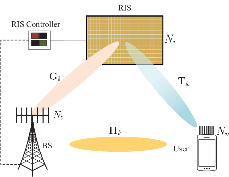
We consider a downlink wideband point-to-point mmWave MIMO communication system as illustrated in Fig. 1, where the BS is equipped with $N_{b}$ antennas and transmits signals to a user with $N_{u}$ antennas, via the help of one $N_{r}$-element RIS. In order to mitigate the spatial-wideband effect of the wideband mmWave channel, OFDM with $K$ subcarriers is employed to modulate the signal at the BS [11, 12]. Let $\mathbf{s}_{k}\in\mathbb{C}^{N_{b}\times 1}$ denote the transmitted signal vector at subcarrier $k$. The transmit covariance matrix at subcarrier $k$ is defined as $\mathbf{Q}_{k}\triangleq\mathbb{E}\{\mathbf{s}_{k}\mathbf{s}_{k}^{H}\}\in\mathbb{C}^{N_{b}\times N_{b}}$, with $\mathbf{Q}_{k}\succeq\mathbf{0}$. The normalized transmit power constraint at the BS is given by

Without loss of generality, we assume the maximum excess delay is of $L_{\text{max}}$ taps in the time domain for the baseband equivalent channels of both the BS-RIS-user reflecting link and the BS-user direct link. The transmit signal $\mathbf{s}_{k}$ is first transformed into the time domain through a $K$-point inverse discrete Fourier transform (IDFT), followed by the appending of a cyclic prefix (CP) of length $N_{\text{CP}}$, with $N_{\text{CP}}\geq L_{\text{max}}$. At the user side, after removing the CP and performing the $K$-point discrete Fourier transform (DFT), the baseband received signal $\mathbf{y}_{k}\in\mathbb{C}^{N_{u}\times 1}$ at the $k$-th subcarrier can be presented as

where $\mathbf{T}_{k}\in\mathbb{C}^{N_{u}\times N_{r}}$, $\mathbf{G}_{k}\in\mathbb{C}^{N_{r}\times N_{b}}$, and $\mathbf{H}_{k}\in\mathbb{C}^{N_{u}\times N_{b}}$ denote the frequency-domain channel on subcarrier $k$ from the RIS to the user, from the BS to the RIS, and from the BS to the user, respectively; $\mathbf{\Theta}\in\mathbb{C}^{N_{r}\times N_{r}}$ denotes the response matrix at the RIS, which is written as

where $\theta_{i}\in[0,2\pi)$ and $\xi_{i}\in[0,1]$ represent the phase shift and the amplitude of the reflection coefficient of the $i$-th reflection unit, respectively; and $\mathbf{n}_{k}\thicksim\mathcal{C}\mathcal{N}{(\mathbf{0},\sigma^{2}\mathbf{I}_{N_{u}})}$ represents the additive white Gaussian noise vector with zero mean and variance $\sigma^{2}$ ²² 2 Without loss of generality, the variances of noise at different subcarriers are assumed to be the same.. Note that the RIS can only bring the same phase shift on different subcarriers due to the lack of the ability of digital signal processing ³³ 3 In this paper, we assume that the RIS units are frequency independent as widely adopted in the existing literature [13, 15, 16, 17, 18, 14, 19, 20, 21, 22, 23, 24, 25]. Some literature, e.g., [27], studies the property of the frequency dependency of RIS. Nevertheless, there is still lack of a general model to accurately characterize the nonlinear response of RIS over various frequencies. [15]. In addition, the amplitude $\xi_{i},\forall i\in\mathcal{N}_{r}$ is assumed to be one to maximize the signal reflection and simplify the hardware design of the RIS [6, 17, 13]. Let $\mathcal{K}=\{1,\ldots,K\}$ and $\mathcal{N}_{r}=\{1,\ldots,N_{r}\}$ denote the index sets of subcarriers and RIS elements, respectively.

Due to the limited scattering paths in mmWave channels, the SV model is widely adopted for modelling the wideband mmWave channel. Suppose uniform linear arrays (ULAs) are equipped at the BS and the user, and a uniform planar array (UPA) is equipped at the RIS. The frequency domain channel matrix $\mathbf{H}_{k}$, $\mathbf{G}_{k}$ and $\mathbf{T}_{k}$ at subcarrier $k$ can be expressed as [11, 12, 28, 29, 30]

where $L_{h}$ $(L_{g},L_{t})$ is the number of the paths between the BS and the user (the BS and the RIS, the RIS and the user); $\alpha_{h,i}\sim\mathcal{CN}(0,\sigma^{2}_{h,i})$ $(\alpha_{g,i}\sim\mathcal{CN}(0,\sigma^{2}_{g,i}),\alpha_{t,i}\sim\mathcal{CN}(0,\sigma^{2}_{t,i})$ ⁴⁴ 4 In mmWave MIMO communication systems, the complex gain is widely assumed to be i.i.d. random variables following the complex Gaussian distribution [28, 31]. denotes the complex gain of the $i$-th path and assume $\sigma^{2}_{h,1}\geq\sigma^{2}_{h,2}\geq\ldots\geq\alpha_{h,L_{h}}^{2}$ $(\sigma^{2}_{g,1}\geq\sigma^{2}_{g,2}\geq\ldots\geq\alpha_{g,L_{g}}^{2}$, $\sigma^{2}_{t,1}\geq\sigma^{2}_{t,2}\geq\ldots\geq\alpha_{t,L_{t}}^{2})$; $\tau_{h,i}$ $(\tau_{g,i},\tau_{t,i})$ is the delay of the $i$-th path; $f_{k}$ is the frequency at subcarrier $k$, which is given by

where $f_{c}$ is the carrier frequency and $f_{s}$ is the bandwidth. Note that in the narrowband communication systems, it is assumed that $f_{k}=f_{c}$. However, this assumption is invalid in wideband communication systems and will dramatically affect the ergodic achievable rate. $\mathbf{a}_{r}(\cdot)$ $(\mathbf{a}_{t}(\cdot))$ denotes the normalized array response vector at the receiver side (the transmitter side); $\psi_{h,u,i}$ ($\psi_{t,u,i}$) denotes the angle of arrival (AoA) associated with the user of the direct link (the reflecting link); $\psi_{h,b,i}$ ($\psi_{g,b,i}$) denotes the angle of departure (AoD) associated with the BS of the direct link (the reflecting link); $\phi_{g,r,i}$ ($\phi_{t,r,i}$) and $\varphi_{g,r,i}$ ($\varphi_{t,r,i}$) denote the azimuth and elevation angles of the arrival (departure) associated with the RIS. For a ULA with $N$ antennas at the frequency $f_{k}$, the normalized array response vector is given by

where $c$ represents the speed of light, $d=\frac{c}{2f_{c}}=\frac{\lambda}{2}$ is the antenna spacing, $\lambda$ represents the signal wavelength of the central frequency, and $\psi$ denotes the AoA or AoD. For a UPA with $M=M_{y}\times M_{z}$ elements at the frequency $f_{k}$, the normalized array response vector can be expressed as

where $d_{r}$ is the unit cell spacing which is assumed to be half wavelength, $\phi$ and $\varphi$ denote the azimuth and elevation angles, respectively. Defining $\mathbf{A}_{uh,k}=\left[\mathbf{a}_{r}(\psi_{h,u,1},f_{k}),\ldots,\mathbf{a}_{r}(\psi_{h,u,L_{h}},f_{k})\right]\in\mathbb{C}^{N_{u}\times L_{h}}$, $\mathbf{A}_{bh,k}=\left[\mathbf{a}_{t}(\psi_{h,b,1},f_{k}),\mathbf{a}_{t}(\psi_{h,b,2},f_{k}),\ldots,\mathbf{a}_{t}(\psi_{h,b,L_{h}},f_{k})\right]\in\mathbb{C}^{N_{b}\times L_{h}}$, and $\mathbf{H}_{L,k}=\sqrt{\frac{N_{u}N_{b}}{L_{h}}}\text{diag}(\alpha_{h,1}e^{-j2\pi\tau_{h,1}f_{k}},\linebreak\alpha_{h,2}e^{-j2\pi\tau_{h,2}f_{k}},\ldots,\alpha_{h,L_{h}}e^{-j2\pi\tau_{h,L_{h}}f_{k}})$, the channel matrix $\mathbf{H}_{k}$ in (4) can be rewritten as

Defining $\mathbf{A}_{rg,k}=[\mathbf{a}_{r}(\phi_{g,r,1},\varphi_{g,r,1},f_{k}),\linebreak\mathbf{a}_{r}(\phi_{g,r,2},\varphi_{g,r,2},f_{k}),\ldots,\mathbf{a}_{r}(\phi_{g,r,L_{g}},\varphi_{g,r,L_{g}},f_{k})]\in\mathbb{C}^{N_{r}\times L_{g}}$, $\mathbf{A}_{bg,k}=\left[\mathbf{a}_{t}(\psi_{g,b,1},f_{k}),\ldots,\mathbf{a}_{t}(\psi_{g,b,L_{g}},f_{k})\right]\in\mathbb{C}^{N_{b}\times L_{g}}$, and $\mathbf{G}_{L,k}=\sqrt{\frac{N_{r}N_{b}}{L_{g}}}\text{diag}(\alpha_{g,1}e^{-j2\pi\tau_{g,1}f_{k}},\alpha_{g,2}e^{-j2\pi\tau_{g,2}f_{k}},\linebreak\ldots,\alpha_{g,L_{g}}e^{-j2\pi\tau_{g,L_{g}}f_{k}})$, the channel matrix $\mathbf{G}_{k}$ in (5) can be expressed as

Defining $\mathbf{A}_{rt,k}=[\mathbf{a}_{t}(\phi_{t,r,1},\varphi_{t,r,1},f_{k}),\linebreak\mathbf{a}_{t}(\phi_{t,r,2},\varphi_{t,r,2},f_{k}),\ldots,\mathbf{a}_{t}(\phi_{t,r,L_{t}},\varphi_{t,r,L_{t}},f_{k})]\in\mathbb{C}^{N_{r}\times L_{t}}$, $\mathbf{A}_{ut,k}=[\mathbf{a}_{r}(\psi_{t,u,1},f_{k}),\ldots,\mathbf{a}_{r}(\psi_{t,u,L_{t}},f_{k})]\in\mathbb{C}^{N_{u}\times L_{t}}$, and $\mathbf{T}_{L,k}=\sqrt{\frac{N_{r}N_{u}}{L_{t}}}\text{diag}(\alpha_{t,1}e^{-j2\pi\tau_{t,1}f_{k}},\alpha_{t,2}e^{-j2\pi\tau_{t,2}f_{k}},\linebreak\ldots,\alpha_{t,L_{t}}e^{-j2\pi\tau_{t,L_{t}}f_{k}})$, the channel matrix $\mathbf{T}_{k}$ in (6) can be presented as

For a given transmit covariance matrix $\{\mathbf{Q}_{k}\}_{k=1}^{K}$ and a given RIS response matrix $\mathbf{\Theta}$, the ergodic achievable rate of the RIS-assisted mmWave MIMO-OFDM communication system is given by

where $P_{T}>0$ is the power budget at the BS, and $\mathbf{H}_{\text{eff},k}=\mathbf{T}_{k}\mathbf{\Theta}\mathbf{G}_{k}+\mathbf{H}_{k}$ denotes the effective channel at subcarrier $k$ between the BS and the user. The expectation is taken over the effective channel $\mathbf{H}_{\text{eff}}$. More specifically, it is taken over the complex channel gains $\{\alpha_{h,i}\}_{i=1,2,\ldots,L_{h}}$ in Eq. (4), $\{\alpha_{g,i}\}_{i=1,2,\ldots,L_{g}}$ in Eq. (5), and $\{\alpha_{t,i}\}_{i=1,2,\ldots,L_{t}}$ in Eq. (6). In this paper, we aim to maximize the ergodic achievable rate by jointly designing the transmit covariance matrix $\{\mathbf{Q}_{k}\}_{k=1}^{K}$ at the BS and the response matrix $\mathbf{\Theta}$ at the RIS, subject to the maximum power budget at the BS. Therefore, the optimization problem can be formulated as

The problem $\mathcal{P}_{0}$ is highly challenging mainly due to the following three facts. First of all, there is no explicit expression of the ergodic achievable rate and the expectation operation in Eq. (13) prevents further optimization. Secondly, the problem is non-convex due to the unit-modulus constraints of the RIS, and thus difficult to be optimally solved. Last but not the least, different from the narrowband communication systems, the RIS can only apply the same phase shifts over different subcarriers. Thereby, we need to consider all of the subcarriers when designing the RIS. In the following, we will firstly find an explicit expression to approximate the ergodic achievable rate in Section III, and then maximize the ergodic achievable rate by jointly designing $\{\mathbf{Q}_{k}\}_{k=1}^{K}$ and $\mathbf{\Theta}$ in Section IV.

The derivation of the ergodic achievable rate is much more difficult than that in our previous work [26], where the direct link is blocked by obstacles. In the previous work, [32, Theorem 9.H.1.a] is frequently adopted during the derivation. However, when the direct BS-user link exists, the cross product term $\mathbf{H}_{k}\mathbf{Q}_{k}\mathbf{G}_{k}^{H}\mathbf{\Theta}^{H}\mathbf{T}_{k}^{H}$ of the ergodic achievable rate is not a positive semi-definite Hermitian matrix, which prevents further derivation. Fortunately, we have the following proposition.

The expectation operation in (17) hinders further optimization. To overcome this difficulty, Jensen’s inequality is adopted to obtain simplified expressions.

In this subsection, we investigate the tightness of the approximations via numerical results. Let us first consider the details of the channels as illustrated in Section II-B. The central carrier frequency is $f_{c}=28$ GHz, the number of subcarriers is $K=24$, the length of CP is $N_{CP}=10$, and the bandwidth is $f_{s}=1$ GHz. The angles $\psi_{h,b,i}$, $\psi_{g,b,i}$, $\psi_{h,u,i}$ and $\psi_{t,u,i}$ are randomly generated and uniformly distributed in $[-\pi,\pi)$, $\phi_{g,r,i}$ and $\phi_{t,r,i}$ in $[-\pi/2,\pi/2]$, and $\varphi_{g,r,i}$ and $\varphi_{t,r,i}$ in $[0,\pi]$. The exponential distribution is adopted to model the variances of the complex gain [34]. In order to make the complex gain of the direct link and the reflecting link comparable, we set $\sigma_{h,i}^{2}\sim\exp(1)$, $\sigma_{g,i}^{2}\sim\exp(0.1)$ and $\sigma_{t,i}^{2}\sim\exp(0.1)$. All curves are averaged over 100 sets of independent realizations of the angles. For each set of angle realization, 1000 independent realizations of the path gains are generated for the Monte-Carlo simulations. Here, the phase matrix of RIS is randomly generated. We investigate the ergodic achievable rate against SNR with different numbers of antennas or reflection units (where $\mathbf{Q}_{k}$ is generated according to Eq. (19), $\mathbf{\Lambda}_{q,k}=\frac{1}{KN_{s}}\mathbf{I}_{N_{s}}$, and $L_{g}=L_{t}=L_{h}=6$), different number of paths (where $\mathbf{Q}_{k}$ is generated according to Eq. (19), $\mathbf{\Lambda}_{q,k}=\frac{1}{KN_{s}}\mathbf{I}_{N_{s}}$, $N_{b}=100$, $N_{r}=169$, and $N_{u}=16$), and different transmit covariance matrices (where $L_{g}=L_{t}=L_{h}=6$, $N_{b}=100$, $N_{r}=169$, $N_{u}=16$, $\mathbf{Q}_{1}$ is generated according to Eq. (19), $\mathbf{\Lambda}_{q,k}=\frac{1}{KN_{s}}\mathbf{I}_{N_{s}}$, and $\mathbf{Q}_{2}=\frac{1}{KN_{b}}\mathbf{I}_{N_{b}}$) in Fig. 3, 3, and 4, respectively. In addition, we compare the normalized error of $R_{Jen}\left(\{\mathbf{Q}_{k}\}_{k=1}^{K},\mathbf{\Theta}\right)$ and $\widetilde{R}\left(\{\mathbf{Q}_{k}\}_{k=1}^{K},\mathbf{\Theta}\right)$ with respect to ${R}\left(\{\mathbf{Q}_{k}\}_{k=1}^{K},\mathbf{\Theta}\right)$ when $\text{SNR}=20$ dB in Table I. From Figs. 3-4 and Table I, we find that the approximations $R_{Jen}\left(\{\mathbf{Q}_{k}\}_{k=1}^{K},\mathbf{\Theta}\right)$ and $\widetilde{R}\left(\{\mathbf{Q}_{k}\}_{k=1}^{K},\mathbf{\Theta}\right)$ are close to ${R}\left(\{\mathbf{Q}_{k}\}_{k=1}^{K},\mathbf{\Theta}\right)$ when the number of paths is one, i.e., $L_{g}=L_{t}=L_{h}=1$. The approximations are larger than the actual results in other cases. It is mainly due to the following three facts. First of all, Proposition 1 utilizes the asymptotic orthogonality of array response vectors. However, the number of antennas at the BS is usually limited in practice, which leads to $\mathbf{G}_{k}\mathbf{H}_{k}^{H}\neq\mathbf{0}^{N_{r}\times N_{u}}$. Second, the optimal $\mathbf{Q}_{k}$ is closely related to the end-to-end instantaneous channel $\mathbf{H}_{\text{eff},k}$, but only the statistical CSI is available. Thus, the adopted transmit covariance matrix $\mathbf{Q}_{k}$ in Eq. (19) is sub-optimal, resulting in some errors. Third, $R_{Jen}\left(\{\mathbf{Q}_{k}\}_{k=1}^{K},\mathbf{\Theta}\right)$ is amplified by the Jensen’s inequality. Nevertheless, the trend of the derived approximations is consistent with the actual ergodic achievable rate, and it will be shown later that our proposed algorithm outperforms the algorithm in [9].

References

- [1] T. S. Rappaport, S. Sun, R. Mayzus, H. Zhao, Y. Azar, K. Wang, G. N. Wong, J. K. Schulz, M. Samimi, and F. Gutierrez, “Millimeter wave mobile communications for 5G cellular: It will work!” IEEE Access, vol. 1, pp. 335–349, 2013.
- [2] R. W. Heath, N. Gonzalez-Prelcic, S. Rangan, W. Roh, and A. M. Sayeed, “An overview of signal processing techniques for millimeter wave MIMO systems,” IEEE J. Sel. Topics Signal Process., vol. 10, no. 3, pp. 436–453, 2016.
- [3] Q. Wu and R. Zhang, “Towards smart and reconfigurable environment: Intelligent reflecting surface aided wireless network,” IEEE Commun. Mag., vol. 58, no. 1, pp. 106–112, Jan. 2020.
- [4] S. Gong, X. Lu, D. T. Hoang, D. Niyato, L. Shu, D. I. Kim, and Y.-C. Liang, “Toward smart wireless communications via intelligent reflecting surfaces: A contemporary survey,” IEEE Commun. Surv. Tutor., vol. 22, no. 4, pp. 2283–2314, Jun. 2020.
- [5] R. Alghamdi, R. Alhadrami, D. Alhothali, H. Almorad, A. Faisal, S. Helal, R. Shalabi, R. Asfour, N. Hammad, A. Shams, N. Saeed, H. Dahrouj, T. Y. Al-Naffouri, and M.-S. Alouini, “Intelligent surfaces for 6G wireless networks: A survey of optimization and performance analysis techniques,” IEEE Access, vol. 8, pp. 202 795–202 818, Oct. 2020.
- [6] Q. Wu and R. Zhang, “Intelligent reflecting surface enhanced wireless network via joint active and passive beamforming,” IEEE Trans. Wireless Commun., vol. 18, no. 11, pp. 5394–5409, Nov. 2019.
- [7] H. Guo, Y.-C. Liang, J. Chen, and E. G. Larsson, “Weighted sum-rate maximization for reconfigurable intelligent surface aided wireless networks,” IEEE Trans. Wireless Commun., vol. 19, no. 5, pp. 3064–3076, May 2020.
- [8] S. Zhang and R. Zhang, “Capacity characterization for intelligent reflecting surface aided MIMO communication,” IEEE J. Sel. Areas Commun., vol. 38, no. 8, pp. 1823–1838, Aug. 2020.
- [9] P. Wang, J. Fang, L. Dai, and H. Li, “Joint transceiver and large intelligent surface design for massive MIMO mmwave systems,” IEEE Trans. Wireless Commun., vol. 20, no. 2, pp. 1052–1064, Feb. 2021.
- [10] Huawei 6G White Paper, “6G The Next Horizon,” 2021. [Online]. Available: https://www-file.huawei.com/-/media/corp2020/pdf/tech-insights/1/6g-white-paper-cn.pdf?la=zh.
- [11] B. Wang, F. Gao, S. Jin, H. Lin, and G. Y. Li, “Spatial- and frequency-wideband effects in millimeter-wave massive MIMO systems,” IEEE Trans. Signal Process., vol. 66, no. 13, pp. 3393–3406, Jul. 2018.
- [12] B. Ning, Z. Tian, Z. Chen, C. Han, J. Yuan, and S. Li, “Prospective beamforming technologies for ultra-massive MIMO in terahertz communications: A tutorial,” 2021. [Online]. Available: https://arxiv.org/abs/2107.03032
- [13] S. Ma, W. Shen, J. An, and L. Hanzo, “Wideband channel estimation for IRS-aided systems in the face of beam squint,” IEEE Trans. Wireless Commun., vol. 20, no. 10, pp. 6240–6253, 2021.
- [14] Y. Chen, D. Chen, and T. Jiang, “Beam-squint mitigating in reconfigurable intelligent surface aided wideband mmwave communications,” in Proc. IEEE WCNC, Apr. 2021, pp. 1–6.
- [15] Y. Yang, B. Zheng, S. Zhang, and R. Zhang, “Intelligent reflecting surface meets OFDM: Protocol design and rate maximization,” IEEE Trans. Commun., vol. 68, no. 7, pp. 4522–4535, Jul. 2020.
- [16] Y. Yang, S. Zhang, and R. Zhang, “IRS-enhanced OFDMA: Joint resource allocation and passive beamforming optimization,” IEEE Wireless Commun. Lett., vol. 9, no. 6, pp. 760–764, Jun. 2020.
- [17] B. Zheng and R. Zhang, “Intelligent reflecting surface-enhanced OFDM: Channel estimation and reflection optimization,” IEEE Wireless Commun. Lett., vol. 9, no. 4, pp. 518–522, 2020.
- [18] Z. He, H. Shen, W. Xu, and C. Zhao, “Low-cost passive beamforming for RIS-aided wideband OFDM systems,” IEEE Wireless Commun. Lett., vol. 11, no. 2, pp. 318–322, 2022.
- [19] H. Li, R. Liu, M. Liy, Q. Liu, and X. Li, “IRS-enhanced wideband MU-MISO-OFDM communication systems,” in Proc. IEEE WCNC, May 2020, pp. 1–6.
- [20] P. Nuti, E. Balti, and B. L. Evans, “Spectral efficiency optimization for mmwave wideband MIMO RIS-assisted communication,” in 2022 IEEE 95th Vehicular Technology Conference: (VTC2022-Spring), 2022, pp. 1–6.
- [21] K. Ying, Z. Gao, S. Lyu, Y. Wu, H. Wang, and M.-S. Alouini, “GMD-based hybrid beamforming for large reconfigurable intelligent surface assisted millimeter-wave massive MIMO,” IEEE Access, vol. 8, pp. 19 530–19 539, Jan. 2020.
- [22] S. H. Hong, J. Park, S.-J. Kim, and J. Choi, “Hybrid beamforming for intelligent reflecting surface aided millimeter wave MIMO systems,” IEEE Trans. Wireless Commun., pp. 1–1, 2022.
- [23] Z. Zhang and L. Dai, “A joint precoding framework for wideband reconfigurable intelligent surface-aided cell-free network,” IEEE Trans. Signal Process., vol. 69, pp. 4085–4101, Jun. 2021.
- [24] W. Jiang, B. Chen, S. Garg, J. Nie, J. Zhao, and Z. Xiong, “Joint transmit precoding and reflect beamforming for IRS-assisted MIMO-OFDM secure communications,” in Proc. IEEE GLOBECOM, Dec. 2021, pp. 1–6.
- [25] W. Jiang, B. Chen, J. Zhao, Z. Xiong, and Z. Ding, “Joint active and passive beamforming design for the IRS-assisted MIMOME-OFDM secure communications,” IEEE Trans. Veh. Technol., vol. 70, no. 10, pp. 10 369–10 381, Oct. 2021.
- [26] R. Li, S. Sun, Y. Chen, C. Han, and M. Tao, “Ergodic achievable rate analysis and optimization of RIS-assisted millimeter-wave MIMO communication systems,” IEEE Trans. Wireless Commun., pp. 1–1, 2022.
- [27] H. Li, W. Cai, Y. Liu, M. Li, Q. Liu, and Q. Wu, “Intelligent reflecting surface enhanced wideband MIMO-OFDM communications: From practical model to reflection optimization,” IEEE Trans. Commun., vol. 69, no. 7, pp. 4807–4820, 2021.
- [28] X. Yu, J.-C. Shen, J. Zhang, and K. B. Letaief, “Alternating minimization algorithms for hybrid precoding in millimeter wave MIMO systems,” IEEE J. Sel. Topics Signal Process., vol. 10, no. 3, pp. 485–500, Apr. 2016.
- [29] Y. Chen, D. Chen, T. Jiang, and L. Hanzo, “Channel-covariance and angle-of-departure aided hybrid precoding for wideband multiuser millimeter wave MIMO systems,” IEEE Trans. Commun., vol. 67, no. 12, pp. 8315–8328, Dec. 2019.
- [30] M. Wang, F. Gao, S. Jin, and H. Lin, “An overview of enhanced massive MIMO with array signal processing techniques,” IEEE J. Sel. Topics Signal Process., vol. 13, no. 5, pp. 886–901, Sep. 2019.
- [31] A. Alkhateeb, O. El Ayach, G. Leus, and R. W. Heath, “Channel estimation and hybrid precoding for millimeter wave cellular systems,” IEEE J. Sel. Topics Signal Process., vol. 8, no. 5, pp. 831–846, Oct. 2014.
- [32] A. W. Marshall, I. Olkin, and B. C. Arnold, Inequalities: theory of majorization and its applications. Springer, 1979, vol. 143.
- [33] A. Tulino, A. Lozano, and S. Verdu, “Capacity-achieving input covariance for single-user multi-antenna channels,” IEEE Trans. Wireless Commun., vol. 5, no. 3, pp. 662–671, Mar. 2006.
- [34] M. K. Samimi and T. S. Rappaport, “3-D millimeter-wave statistical channel model for 5G wireless system design,” IEEE Trans. Microw. Theory Techn., vol. 64, no. 7, pp. 2207–2225, Jul. 2016.
- [35] P. Almers, F. Tufvesson, O. Edfors, and A. Molisch, “Measured capacity gain using water filling in frequency selective MIMO channels,” in IEEE Int. Symp. Personal, Indoor and Mobile Radio Commun., vol. 3, 2002, pp. 1347–1351 vol.3.
- [36] P.-A. Absil, R. Mahony, and R. Sepulchre, Optimization Algorithms on Matrix Manifolds. Princeton University Press, 2009. [Online]. Available: https://doi.org/10.1515/9781400830244
- [37] J. Chen, “When does asymptotic orthogonality exist for very large arrays?” in Proc. IEEE GLOBECOM, Dec. 2013, pp. 4146–4150.
- [38] X. Yang, X. Li, S. Zhang, and S. Jin, “On the ergodic capacity of mmwave systems under finite-dimensional channels,” IEEE Trans. Wireless Commun., vol. 18, no. 11, pp. 5440–5453, Nov. 2019.