Nonlinear Stochastic Trajectory Optimization for Centroidal Momentum Motion Generation of Legged Robots
Abstract
Generation of robust trajectories for legged robots remains a challenging task due to the underlying nonlinear, hybrid and intrinsically unstable dynamics which needs to be stabilized through limited contact forces. Furthermore, disturbances arising from unmodelled contact interactions with the environment and model mismatches can hinder the quality of the planned trajectories leading to unsafe motions. In this work, we propose to use stochastic trajectory optimization for generating robust centroidal momentum trajectories to account for additive uncertainties on the model dynamics and parametric uncertainties on contact locations. Through an alternation between the robust centroidal and whole-body trajectory optimizations, we generate robust momentum trajectories while being consistent with the whole-body dynamics. We perform an extensive set of simulations subject to different uncertainties on a quadruped robot showing that our stochastic trajectory optimization problem reduces the amount of foot slippage for different gaits while achieving better performance over deterministic planning.
Keywords:
stochastic optimal control, chance-constraints, trajectory optimization, legged robots,
and LAAS-CNRS, Université de Toulouse, CNRS, Toulouse,
and Industrial Engineering Department, University of Trento, Italy,
, and Tandon School of Engineering, New York University, New York, USA,
1 Introduction
Trajectory optimization has become a dominant paradigm for planning and control of whole-body trajectories for legged robots mordatch2012; posa2014; winkler2018; carpentier2021. Despite recent advancements in real-time trajectory re-planning sleiman2021unified; meduri2022biconmp, dealing with uncertainties and assessing risk remains an open challenge in controlling legged robots. Uncertainties arising from inaccurate modelling, estimation errors, etc., might cause the robot to make/break contact at a different contact position and/or timing than the planned trajectory. This often leads to constraint violations in the form of slipping or collision of the robot with its environment causing safety hazards.
Most of the work that took into account uncertainties in the control of legged locomotion mainly resorts to linear models, such as the Linear Inverted Pendulum Model (LIPM). For instance, Villa et al. villa2017 used a tube-based linear Robust Model Predictive Control (RMPC) to plan Center of Mass (CoM) trajectories subject to worst-case disturbances on the Center of Pressure (CoP). To reduce the conservativeness of RMPC, Gazar et al. gazar2020 resorted to linear stochastic MPC subject to stochastic additive disturbances on the dynamics and CoM linear chance-constraints. Yeganegi et al. yeganegi2019 used Bayesian Optimization to learn cost function weights to achieve robust walking motions under different uncertainties. However, assuming fixed height for the CoM and zero angular momentum around the CoM limits the range of motions and cannot plan trajectories in non co-planar multi-contact scenarios.
There has been some effort in the literature to take into account uncertainties in the nonlinear trajectory optimization problem for legged locomotion. In these approaches, Differential Dynamic Programming (DDP) has been the method of choice as it takes into account the structure of the underlying optimal control problem to find the optimal trajectories and control policy tassa2012synthesis; mastalli2020crocoddyl. In an effort to take uncertainties into account, Mordatch et al. mordatch2015 used an offline ensemble DDP enabling them to transfer the whole-body trajectories to a real humanoid robot. Recently, Hammoud et al. hammoud2021 used a risk-sensitive version of DDP to optimize for impedance gains to deal with uncertainties in contact. Despite the appealing convergence properties of DDP-based approaches, inequality constraints can only be considered implicitly in the form of penalties, which makes it difficult to reason about the effect of uncertainties on the constraint satisfaction robustness. Tangent to that work, Darnach et al. drnach2021 used Expected Residual Minimization (ERM) to solve a contact-implicit stochastic complementarity problem. However, contact-implicit trajectory optimization can be quite hard to tune, computationally demanding, and gets easily stuck in local minimas. A middle-ground model between whole body and template models for legged locomotion is the centroidal momentum dynamics orin2008. While this model captures the dynamics between the external forces and the centroidal states exactly wieber2016, it is relatively low dimensional and the nonlinearity structure in the model is well understood herzog2016structured. Hence, it is more tractable to use direct methods with explicit consideration of the force and CoM constraints and design force trajectories that are robust to the different types of uncertainties in the model. In this work, we propose to solve stochastic trajectory optimization problems for centroidal momentum generation of legged robots in the presence of additive uncertainties in the model dynamics and uncertainties in the contact location. We write down the friction cone constraints as chance constraints and study the effect of the uncertainties on the satisfaction of these constraints. Our work is related to brasseur2015robust; dai2016planning, where the motion of the CoM was restricted within certain bounds to make the underlying optimal control problem convex. In our work instead, we take into account different types of realistic uncertainties in the trajectory optimization problem to find trajectories that are robust against them and are better transferable to the real world. Moreover, compared to brasseur2015robust; dai2016planning, we construct the problem as a stochastic optimization rather than Min-max formulation which is a less conservative formulation and facilitates the generation of more complex behaviours.
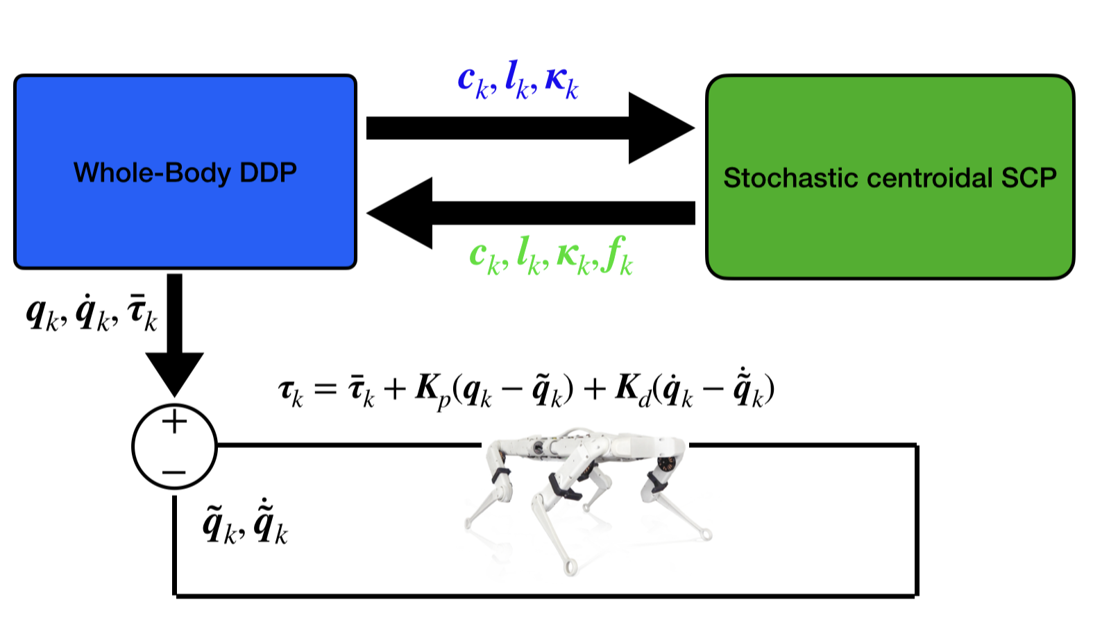
Our main contributions are: 1) We propose to use stochastic trajectory optimization using Sequential Convex Programming (SCP) for generating robust centroidal momentum trajectories subject to additive uncertainties in the dynamics, as well as parametric contact position uncertainties. 2) By considering chance constraints on the friction cones, this is the first work (to the best of our knowledge) that designs controllers for legged robots that generates robust force trajectories subject to contact location uncertainty. In the same spirit as herzog2016structured, we propose a whole-body trajectory planning framework that alternates between whole-body motion planning and centroidal momentum planning. Contrary to herzog2016structured—but similarly to budhiraja2019dynamics—we use whole-body DDP instead of a kinematics optimization, and use the solution to warm-start the stochastic SCP centroidal momentum solver. The resulting (robust) momentum trajectories are later used by the whole-body DDP again to track the resulting robust centroidal trajectories and contact force trajectories. This way, we make sure that the generated momentum trajectories are robust while being consistent with the robot whole-body dynamics. 3) Finally, we run 400 Monte-carlo simulations on the open-source quadruped robot Solo grimminger2020open in a Pybullet simulation environment coumans2016pybullet for dynamic trotting and bounding gaits while applying different disturbances. We show that Stochastic trajectory optimization is able to complete all the motions safely while reducing feet slippage, and achieving better centroidal tracking performance over the deterministic planning 11 1 submission video..
2 Background
2.1 Notation
A random variable following a distribution is denoted as , with being the expected value of , and . The weighted norm is denoted as .
2.2 Robot Dynamics
The full-body dynamics of a floating-base robot in contact with the environment can be derived using Euler-Lagrange equations of motion as follows wieber2016:
| (1) |
where represents the generalized robot position characterizing the robot’s floating base pose (position and orientation) w.r.t. an inertial frame , and the joint positions respectively. denotes the inertia matrix, and is the vector capturing the Coriolis, centrifugal, gravity and joint friction forces. is the associated jacobian of the -th end-effector wrench acting on the environment. Finally, is the selector matrix of the actuated joint torques . We can further split (1) into its under-actuated and actuated parts;
| (2a) | ||||
| (2b) | ||||
By writing down the floating-base dynamics for the CoM instead of the floating base position , we obtain the following relationship between the centroidal momentum dynamics and the generalized velocities
| (3) |
via the Centroidal Momentum Matrix (CMM) orin2008. The angular and linear momenta are denoted as and respectively. Given (3), we are interested in planning desired centroidal momentum trajectories that satisfy the following Newton-Euler dynamics:
| (4) |
where represents the robot’s CoM, at which the total mass of the robot is concentrated. is the -th end-effector’s contact position, with being the local Center of Pressure (CoP). and represent end-effector’s contact forces and torque for flat-footed robots, respectively. The rotation matrix captures the contact normals mapping quantities from the -th end-effector’s frame to the inertial frame. Note that for point-footed robots, which we consider from now on, and are always null, but the same analysis still holds for flat-footed robots.
2.3 Centroidal Momentum Trajectory Optimization
First we present the deterministic nonlinear discrete-time optimal control problem (OCP) for centroidal momentum trajectory optimization with fixed contact position and timing.
Problem 1.
Nominal Optimal Control Problem (NOCP)
| (5a) | ||||
| s.t. | ||||
| (5b) | ||||
| (5c) | ||||
| (5d) | ||||
| (5e) | ||||
| (5f) | ||||
| (5g) | ||||
| (5h) | ||||
where with , and with are the states and control optimizers along the control horizon N. The centroidal momentum dynamics are discretized with a time-step using an explicit Euler integration scheme (5b), where (5f)-(5g) represents the initial and final conditions respectively. In order to avoid contact slippage, the local contact forces in the end-effector frame () are constrained inside the linearized friction cone constraints (5c)-(5d), where the static coefficient of friction is denoted as with the vertical component of the force being positive. Finally, the CoM is constrained to be within the leg length reachability limits (5e).
3 Stochastic Optimal Control for Centroidal Momentum Trajectory Optimization
In this section we present a stochastic version of problem (1) that takes into account additive stochastic uncertainties on the centroidal momentum dynamics as well as contact position uncertainties subject to friction pyramid chance constraints. We consider the following discrete-time stochastic nonlinear OCP:
Problem 2.
Stochastic Optimal Control Problem (SOCP)
| (6a) | ||||
| s.t. | ||||
| (6b) | ||||
| (6c) | ||||
| (6d) | ||||
| (6e) | ||||
| (6f) | ||||
| (6g) | ||||
With an abuse of notation from Problem (1), and will be considered the stochastic state and control policies evolving according to the parametric and additive stochastic disturbance realizations , and . (6c)-(6d) are the state and control polytopic joint chance constraints with and being the probability levels of state and control constraint satisfaction respectively.
Assumption 1.
(i.i.d. Gaussian disturbances)
, and are assumed to be independent and identically distributed (i.i.d.) disturbance realisations following Gaussian distributions. , and represent the mean and covariance of the contact positions respectively. and are the mean and covariance of the additive noise on the centroidal dynamics.
3.1 Individual Chance Constraints Reformulation
Solving the above joint chance constraints (6c)-(6d) involves the integration of multi-dimensional Gaussian Probability Density Functions (PDFs), which becomes computationally intractable for high dimensions. One effective solution is to use Boole’s inequality:
| (7) |
as a conservative union bound on the joint chance constraints Ono2010. We can rewrite the complement of the state chance constraints as a conjunction of individual chance constraints as follows:
which can be written conservatively as
| (8) |
By applying Boole’s inequality on the above equation, and allocating constraint violation risk equally , with being the number of intersecting hyper-planes forming the state joint polytopic constraint, we reach
| (9) |
Similarly, control joint chance constraint (6d) can be reformulated as a set of individual chance constraints following the same arguments as before
| (10) |
where is the equally distributed control constraint risk.
Remark 1.
Allocating risk of constraint violations equally can be quite conservative since one would preferably allocate more risk to active constraints over inactive ones. Another approach can be optimizing for allowable violation for each constraint as in Ma2012, which involves higher computational complexity.
3.2 Deterministic Reformulation of Individual Chance Constraints
Solving the chance constraints (3.1)-(10), requires propagating the uncertainty through the nonlinear dynamics. We adopt a linearization-based covariance propagation as in zhu2019lew2020. Using a state-feedback control policy , where are pre-stabilizing feedback gains, then the mean and covariance of the dynamics evolve as
| (11a) | ||||
| (11b) | ||||
where is the nominal nonlinear dynamics estimated at current mean of the state and controls of the trajectory. , and is the closed-loop dynamics. is the Jacobian of the dynamics w.r.t. the state. is the Jacobian of the dynamics w.r.t. controls. Finally, represents the Jacobian of the dynamics w.r.t. the contact positions.
Remark 2.
Other approaches can be used for uncertainty propagation through nonlinear dynamics like unscented-based transforms plancher2017, or Generalized Polynommial Chaos (gPC) nakka2019. These methods can lead to more accurate estimate of the propagated uncertainty at the cost of significant increase in complexity. Since computational efficiency is more important in our case (especially for online re-planning of the trajectories), we prefer to not use these methods.
Based on Assumption (1) and the covariance propagation in (11b), we seek the least conservative upper bounds on the state and controls individual chance-constraints (6c)-(6d). Using the inverse of the Cumulative Density Function (CDF) of a Gaussian distribution, we arrive to a deterministic reformulation of the chance constraints:
| (12a) | |||
| (12b) | |||
where and are known as the state and control back-off bounds ensuring the satisfaction of the individual chance constraints (6c)-(6d), respectively.
3.3 Deterministic Reformulation of SOCP
Given the previous reformulation of the individual chance constraints, we can write down the following NOCP.
Problem 3.
NOCP with reformulated individual chance-constraints:
| (13a) | ||||
| s.t. | ||||
| (13b) | ||||
| (13c) | ||||
| (13d) | ||||
| (13e) | ||||
| (13f) | ||||
| (13g) | ||||
where (13b) is now the mean of the nonlinear dynamics. In order to solve the the above nonlinear OCP, we resort to Sequential Convex Programming (SCP), which we explain in the next subsection.
3.4 SCP with L1 Trust Region Penalty Cost
SCP attempts to solve nonlinear OCPs by successively linearizing the dynamics, costs and constraints to solve a convex sub-problem at every iteration. The dynamics are linearized with a first-order Taylor expansion around the previous state and control trajectories computed at the -th succession. Successive linearization introduces two well-known problems Ma2012.
1) Artificial infeasibility: the problem becomes infeasible even if the original nonlinear problem is feasible. The most evident example of this arises when the problem is linearized about an unrealistically short time horizon, so that there is no feasible control input that can satisfy the prescribed dynamics and constraints. 2) Artificial unboundedness: the solution takes steps far away from the validity of the linear model. In order to mitigate artificial unboundedness, a trust-region constraint is employed. Different approaches are adapted to tackle artificial infeasiblity. In Ma2012, the authors employ hard constraints and virtual controls as slack variables on the constraints. However, bonalli2019 enforced hard constraints on the dynamics and convex soft penalties on the rest of the constraints along with trust region constraints. In this work we follow the same rationale as bonalli2019; schulman2014, where the trust region constraints are enforced as penalty cost in the form of
| (14a) | |||
| (14b) | |||
where is the trust region radius. Notice that the above penalty cost is exact—meaning that as the penalty weight gets infinitely large, the constraint violations are driven to zero. Even though (14a) is non-differentiable, yet it can be solved efficiently by introducing a slack variable as follows:
| (15a) | ||||
| s.t. | ||||
| (15b) | ||||
| (15c) | ||||
In order to solve problem (3), we solve a sequence of Quadratic Programs (QPs) in problem (4), accompanied by a trust region update mechanism based on the accuracy ratio of the linearized model w.r.t. the nonlinear model as in bonalli2019lew2020.
Problem 4.
Convexified QP at the -th SCP iteration:
| (16a) | ||||
| s.t. | ||||
| (16b) | ||||
| (16c) | ||||
| (16d) | ||||
| (16e) | ||||
| (16f) | ||||
| (16g) | ||||
| (16h) | ||||
| (16i) | ||||
| (16j) | ||||
is the concatenated vector of states and controls at time . Constraints (16e)-(16f) are the linearized state and control chance constraints, where
| (17) |
represents the covariance derivative w.r.t. . Notice that this term is more involved since it includes the propagation of the tensor derivatives of the covariance matrix given the current states and controls as well as the previous states and controls as follows:
| (18) |
We resort to the autodiff library JAX jax2018 for such computation. Finally, the trust region constraints (16g) are enforced only on the angular momentum since it’s the only nonlinear part in the centroidal dynamics.
4 Simulations Results
In this section, we report simulation results for the quadruped robot Solo in the Pybullet simulation environment coumans2016pybullet. We compare trajectories generated using centroidal stochastic trajectory optimization against nominal trajectory optimization for trotting and bounding gaits on challenging unknown cluttered terrains. Offline, we warm start the centroidal SCP solver using centroidal trajectories coming from the whole-body DDP solver Croccodyl mastalli2020crocoddyl. Then, we optimize whole-body trajectories to track back the optimized centroidal and force trajectories from the SCP solver as illustrated pictorially in Fig. 1. The cost weights for both whole-body DDP and centroidal SCP are summarized in Table 1 and Table 2, respectively. Both DDP and SCP solvers were discretized with a sampling time of ms for a planning horizon length of , and motion plans were designed on a flat ground with a floor static coefficient of friction for both solvers.


| DDP solver task weights | ||
|---|---|---|
| Task | Trot | Bound |
| Swing foot | 1e6 | 1e6 |
| SCP CoM tracking | 1e3 | 1e1 |
| SCP centroidal tracking | 1e3 | 1e3 |
| SCP force tracking | 1e2 | 8e1 |
| Friction cone | 2e2 | 2e0 |
| State regulation | 1e-1 | 1e-1 |
| Control regulation | 1e0 | 1e0 |
| Contact impact velocity regulation | 2e1 | 2e1 |
During simulation (i.e. online), whole-body DDP joint-space trajectories were tracked at a higher sampling rate of ms using a PD control law:
| (19) |
where are the DDP optimal feedforward joint torque controls, and represent the DDP optimal joint positions and velocities respectively. Although in theory the optimal DDP gains could be used, it was not transferable in our case for highly dynamic motions, especially with long horizon as the motion diverged quickly. For that reason, we used hand-tuned PD gains for the scenarios described in the following subsection. The chance-constraints hyper parameters of the stochastic SCP were tuned as follows for the trotting and bounding motions: the probability level of friction pyramid constraint violations for every leg is . The covariance of the contact position parametric uncertainties for each foot is set to . The covariance of additive centroidal uncertainties is set to , and for the trotting and bounding motions, respectively.
4.1 Simulations setup
We ran a set of Monte-carlo simulations for two scenarios per motion: Scenario 1) without debris: 100 simulations on flat ground with a reduced floor friction , while applying random lateral force disturbances for 200 ms at the center of the robot’s base link. For trotting motion, we set , . For the bounding motion, we set , . Scenario 2) with debris: 100 simulations with reduced floor friction , while adding unplanned debris of cm height ( of the robot’s leg length) with varying orientations of degrees along x and y directions as shown in Fig. 2 and Fig. 3 for trotting and bounding motions, respectively (please refer to the video for more details).The joint impedances were set to , for the trotting motion, and , for the bounding motion. Further, we apply again random lateral force impulses for 200 ms at the center of the robot’s base.


| SCP solver task weights | ||
|---|---|---|
| Task | Trot | Bound |
| DDP CoM tracking | 1e4 | 1e4 |
| DDP linear momentum tracking | 1e3 | 1e3 |
| DDP angular momentum tracking | 1e5 | 1e5 |
| Lateral force regulation per foot (x-direction) | 1e2 | 1e2 |
| Lateral force regulation per foot (y-direction) | 1e0 | 1e2 |
| Vertical force regulation per foot | 1e1 | 1e1 |
| Initial trust region weight | 1e2 | 1e2 |
The same force disturbances were applied to the nominal and stochastic trajectories, and were sampled from a Gaussian distribution with zero mean and N ( of the robot weight). The force impulse is applied at the same randomly sampled time instance after the first second of the motion. We analyze the robustness of the motions generated using stochastic SCP against their nominal counterpart by evaluating the Normalized cumulative sum of the contact position deviations of the robot feet when a foot is in contact with the ground (i.e. foot slippage), which reflects the saturation of the friction pyramid constraints. The normalized cumulative sum was computed by subtracting the average cumulative sum of the previous samples from the current integral quantity at each point in time. Moreover, we report the centroidal tracking performance between the generated SCP references and the simulated trajectories.
First, we discuss the optimized contact forces generated using nominal and stochastic SCPs, which are later tracked using whole-body DDP. In Fig. 4, we plot the ratio between the norm of the tangential forces and the vertical forces for dynamic trotting and bounding motions. As expected, the forces optimized using stochastic SCP saturate less the friction cones compared to the ones optimized with nominal SCP, especially during single support phases where the solution of the QP is unique. This highlights the contribution of the control back-off magnitudes, which increase along the horizon due to the covariance propagation along the linearized dynamics (16f).
For the trotting motion (Fig. 5), trajectories designed using stochastic SCP (our method) achieved less feet slippage mean ( and for scenario 1 and 2, respectively) than nominal SCP and an improved centroidal tracking performance mean ( and ). The same analysis was carried out for the bounding motion in a more challenging terrain (Fig. 3). As shown in Fig. 6, stochastic SCP trajectories contributed to less feet slippage mean ( and for scenarios 1 and 2, respectively) than nominal SCP, and an improved centroidal tracking performance mean ( and ).


5 Discussion and Conclusions
In this work, we used nonlinear stochastic trajectory optimization for generating robust centroidal momentum trajectories for legged robots that take into account additive uncertainties on the centroidal dynamics as well as parametric uncertainties on the contact positions. We used a linearization-based covariance propagation for resolving the stochastic nonlinear dynamics. Furthermore, we resolved the friction pyramid joint chance constraints by designing proper upper bounds (back-offs) at each point in time on the individual hyper-planes forming the friction pyramid polytopes. Finally, we presented a whole-body trajectory optimization framework that alternates between stochastic centroidal trajectory optimization and whole-body trajectory optimization for generating feasible robust whole-body motions. We used our framework to generate trotting and bounding dynamic gaits for the quadruped robot Solo. We then tracked these trajectories in a Pybullet physics simulator, introducing different disturbance realizations and contact uncertainties. The results show that our approach generated safer motions by contributing to less average contact slippage, as well as improved centroidal tracking performance over deterministic trajectory optimization. Although the current stochastic SCP approach does not require additional optimization variables over a deterministic approach SCP, the computational complexity is relatively higher due to uncertainty propagation and the additional tensor derivatives required for solving the linearized chance-constraints.
Another limitation of the current stochastic SCP approach lies in the accuracy of uncertainties propagation through the linearized dynamics, which might be hindered for long horizons. However, we believe that this might not be an issue in practice when applied in receding horizon fashion. To this end, we plan to extend the current framework to nonlinear stochastic MPC in the future.


References
- (1) Mordatch, I., Todorov, E., Popović, Z.: Discovery of complex behaviors through contact-invariant optimization. ACM Trans. Graph. 31(4) (jul 2012)
- (2) Posa, M., Cantu, C., Tedrake, R.: A direct method for trajectory optimization of rigid bodies through contact. The International Journal of Robotics Research 33(1), 69–81 (2014)
- (3) Winkler, A.W., Bellicoso, C.D., Hutter, M., Buchli, J.: Gait and trajectory optimization for legged systems through phase-based end-effector parameterization. IEEE Robotics and Automation Letters 3(3), 1560–1567 (2018)
- (4) Carpentier, J., Wieber, P.B.: Recent progress in legged robots locomotion control. Current Robotics Reports 2(3), 231–238 (2021)
- (5) Sleiman, J.P., Farshidian, F., Minniti, M.V., Hutter, M.: A unified mpc framework for whole-body dynamic locomotion and manipulation. IEEE Robotics and Automation Letters 6(3), 4688–4695 (2021)
- (6) Meduri, A., Shah, P., Viereck, J., Khadiv, M., Havoutis, I., Righetti, L.: Biconmp: A nonlinear model predictive control framework for whole body motion planning. CoRR abs/2201.07601 (2022), https://arxiv.org/abs/2201.07601
- (7) Villa, N.A., Wieber, P.B.: Model predictive control of biped walking with bounded uncertainties. In: 2017 IEEE-RAS 17th International Conference on Humanoid Robotics (Humanoids). pp. 836–841 (2017)
- (8) Gazar, A., Khadiv, M., Prete, A.D., Righetti, L.: Stochastic and robust mpc for bipedal locomotion: A comparative study on robustness and performance. In: 2020 IEEE-RAS 20th International Conference on Humanoid Robots (Humanoids). pp. 61–68 (2021)
- (9) Yeganegi, M.H., Khadiv, M., Moosavian, S.A.A., Zhu, J.J., Del Prete, A., Righetti, L.: Robust humanoid locomotion using trajectory optimization and sample-efficient learning. In: 2019 IEEE-RAS 19th International Conference on Humanoid Robots (Humanoids). pp. 170–177 (2019)
- (10) Tassa, Y., Erez, T., Todorov, E.: Synthesis and stabilization of complex behaviors through online trajectory optimization. In: 2012 IEEE/RSJ International Conference on Intelligent Robots and Systems. pp. 4906–4913 (2012)
- (11) Mastalli, C., Budhiraja, R., Merkt, W., Saurel, G., Hammoud, B., Naveau, M., Carpentier, J., Righetti, L., Vijayakumar, S., Mansard, N.: Crocoddyl: An efficient and versatile framework for multi-contact optimal control. In: 2020 IEEE International Conference on Robotics and Automation (ICRA). pp. 2536–2542 (2020)
- (12) Mordatch, I., Lowrey, K., Todorov, E.: Ensemble-cio: Full-body dynamic motion planning that transfers to physical humanoids. In: 2015 IEEE/RSJ International Conference on Intelligent Robots and Systems (IROS). pp. 5307–5314 (2015)
- (13) Hammoud, B., Khadiv, M., Righetti, L.: Impedance optimization for uncertain contact interactions through risk sensitive optimal control. IEEE Robotics and Automation Letters 6(3), 4766–4773 (2021)
- (14) Drnach, L., Zhang, J.Z., Zhao, Y.: Mediating between contact feasibility and robustness of trajectory optimization through chance complementarity constraints. Frontiers in Robotics and AI 8 (2021)
- (15) Orin, D.E., Goswami, A.: Centroidal momentum matrix of a humanoid robot: Structure and properties. In: 2008 IEEE/RSJ International Conference on Intelligent Robots and Systems. pp. 653–659 (2008)
- (16) Wieber, P.B., Tedrake, R., Kuindersma, S.: Modeling and Control of Legged Robots, pp. 1203–1234. Springer International Publishing, Cham (2016)
- (17) Herzog, A., Schaal, S., Righetti, L.: Structured contact force optimization for kino-dynamic motion generation. In: 2016 IEEE/RSJ International Conference on Intelligent Robots and Systems (IROS). pp. 2703–2710 (2016)
- (18) Brasseur, C., Sherikov, A., Collette, C., Dimitrov, D., Wieber, P.B.: A robust linear mpc approach to online generation of 3d biped walking motion. In: 2015 IEEE-RAS 15th International Conference on Humanoid Robots (Humanoids). pp. 595–601 (2015)
- (19) Dai, H., Tedrake, R.: Planning robust walking motion on uneven terrain via convex optimization. In: 2016 IEEE-RAS 16th International Conference on Humanoid Robots (Humanoids). pp. 579–586 (2016)
- (20) Budhiraja, R., Carpentier, J., Mansard, N.: Dynamics consensus between centroidal and whole-body models for locomotion of legged robots. In: 2019 International Conference on Robotics and Automation (ICRA). pp. 6727–6733 (2019)
- (21) Grimminger, F., Meduri, A., Khadiv, M., Viereck, J., Wüthrich, M., Naveau, M., Berenz, V., Heim, S., Widmaier, F., Flayols, T., et al.: An open torque-controlled modular robot architecture for legged locomotion research. IEEE Robotics and Automation Letters 5(2) (2020)
- (22) Coumans, E., Bai, Y.: Pybullet, a python module for physics simulation for games, robotics and machine learning. http://pybullet.org (2016–2021)
- (23) Ono, M., Blackmore, L., Williams, B.C.: Chance constrained finite horizon optimal control with nonconvex constraints. In: Proceedings of the 2010 American Control Conference. pp. 1145–1152 (2010)
- (24) Ma, Y., Vichik, S., Borrelli, F.: Fast stochastic mpc with optimal risk allocation applied to building control systems. In: 2012 IEEE 51st IEEE Conference on Decision and Control (CDC). pp. 7559–7564 (2012)
- (25) Zhu, H., Alonso-Mora, J.: Chance-constrained collision avoidance for mavs in dynamic environments. IEEE Robotics and Automation Letters 4(2), 776–783 (2019)
- (26) Lew, T., Bonalli, R., Pavone, M.: Chance-constrained sequential convex programming for robust trajectory optimization. In: 2020 European Control Conference (ECC) (2020)
- (27) Plancher, B., Manchester, Z., Kuindersma, S.: Constrained unscented dynamic programming. In: 2017 IEEE/RSJ International Conference on Intelligent Robots and Systems (IROS). pp. 5674–5680 (2017)
- (28) Nakka, Y.K., Chung, S.J.: Trajectory optimization for chance-constrained nonlinear stochastic systems. In: 2019 IEEE 58th Conference on Decision and Control (CDC). pp. 3811–3818 (2019)
- (29) Bonalli, R., Cauligi, A., Bylard, A., Pavone, M.: Gusto: Guaranteed sequential trajectory optimization via sequential convex programming. In: 2019 International Conference on Robotics and Automation (ICRA). pp. 6741–6747 (2019)
- (30) Schulman, J., Duan, Y., Ho, J., Lee, A., Awwal, I., Bradlow, H., Pan, J., Patil, S., Goldberg, K., Abbeel, P.: Motion planning with sequential convex optimization and convex collision checking. The International Journal of Robotics Research (2014)
- (31) Bradbury, J., Frostig, R., Hawkins, P., Johnson, M.J., Leary, C., Maclaurin, D., Necula, G., Paszke, A., VanderPlas, J., Wanderman-Milne, S., Zhang, Q.: JAX: composable transformations of Python+NumPy programs, http://github.com/google/jax