Optical linear polarization study towards Czernik 3 open cluster at different spatial scales
Abstract
We present the optical linear polarization observation of stars towards the core of the Czernik 3 cluster in the Sloan i-band. The data were obtained using the EMPOL instrument on the 1.2 m telescope at Mount Abu Observatory. We study the dust distribution towards this cluster by combining the results from our polarization observations with the data from Gaia EDR3, WISE, and the HI, 12CO surveys. In addition, we use the polarimetric data of previously studied clusters within 15∘ of Czernik 3 to understand the large scale dust distribution. The observational results of Czernik 3 show a large range in the degree of polarization, indicating that the dust is not uniformly distributed over the plane of the sky, even on a small scale. The distance to the Czernik 3 is constrained to kpc using the member stars in the core region identified from Gaia EDR3 astrometry. This makes it one of the most distant clusters observed for optical polarization so far. The variation of observed degree of polarization and extinction towards this cluster direction suggest the presence of at least two dust layers along this line of sight at distances of kpc and kpc. There is an indication of the presence of dust in the centre of the cluster as seen from an increase in the degree of polarization and WISE W4 flux. The large scale distribution of dust reveals the presence of a region of low dust content between the local arm and the Perseus arm.
Keywords:
(ISM:) dust, extinction- ISM: general- (Galaxy:) open clusters and associations: individual (Czernik 3)-methods: observational- techniques: polarimetricI Introduction
Dust is an integral part of the interstellar medium (ISM) and is present everywhere in the sky. Polarization and the extinction of star light are manifestations of the dust in the ISM. Starlight polarization by the interstellar dust is considered as a useful tool to determine the properties of the ISM, e.g., the geometry of the magnetic field at small scale (Goodman et al. 1990) as well as large scale (Mathewson & Ford 1971; Axon & Ellis 1976; Berdyugin et al. 2014; Clemens et al. 2020); grain properties: size, shape, chemical composition and grain efficiency (Mathis 1986; Kim & Martin 1994; Kim & Martin 1995; Clayton et al. 2003; Voshchinnikov & Das 2008; Papoular 2018). Besides this, polarization can also be used to evaluate the dust distribution along the line of sight (Eswaraiah et al. 2012, e.g.,). The dust distribution in the Galaxy can be inferred from extinction properties of the dust as well. Many attempts have been made to construct 3-dimensional extinction maps of the Milky Way galaxy (Lallement et al. 2019; Green et al. 2019, etc). However, these extinction maps are based on models and assumptions. Hence these maps have an inherent bias. On the other hand, polarization measurements give the direct observational signature of dust patches along the line of sight.
Open clusters are important constituents of the Galactic disk and their distribution has been studied to trace the spiral arm structure of the Galaxy (Castro-Ginard et al. 2021; Hao et al. 2021, etc). They are good candidates to carry out the polarization observations as all the member stars have common properties in terms of their distance, age, and proper motion. Polarization data of different clusters will help to study the dust distribution in the Galactic disk particularly the spiral arms. Cluster polarization studies have been used to identify cluster members (Medhi & Tamura 2013) and to understand the dust properties (e.g., Medhi et al. 2008; Eswaraiah et al. 2011; Eswaraiah et al. 2012; Topasna et al. 2018; Singh et al. 2020; Singh & Pandey 2020, and references therein). Linear polarization study of open clusters combined with the distance information from Gaia early data release 3 (Gaia Collaboration et al. 2021, EDR3, ) can help to trace the dust distribution.
In this paper, we present a polarimetric study towards the core of the open cluster Czernik 3 [ and (Dias et al. 2002)]. The cluster is located in the 2nd Galactic quadrant (). Previous studies have provided a range of ages (e.g., 100 Myr: Dias et al. 2002; 630 Myr: Kharchenko et al. 2016; 115 Myr: Bisht et al. 2017), photometric distances (1.4-1.75 kpc), reddening E(B-V) (0.99-1.4 mag), and average extinction mag (Dias et al. 2002; Bisht et al. 2017; Kharchenko et al. 2016). Recently, Cantat-Gaudin et al. 2018 have derived basic parameters and membership of 1229 Galactic open clusters using parallax and proper motion information from Gaia DR2. They showed that this cluster has 48 members with membership probability 0.5, and about half of the member stars of this cluster lie within a radial distance of . They also estimated the most probable distance to the cluster to be 4.47 kpc. Czernik 3 cluster has an extended morphology (Sharma et al. 2020) with a radius of the core and the whole cluster and , respectively (Dias et al. 2002; Kharchenko et al. 2016; Joshi et al. 2016; Bisht et al. 2017; Sharma et al. 2020). Sharma et al. 2020 have placed the cluster at an average distance of kpc. They have claimed that it is a disintegrating old cluster with an average age of Gyr. Thus, there is a large variation in the possible ages and distances to this cluster. Astrometric data from Gaia EDR3 is expected to help better constrain the distance and membership.
The aim of our study is to understand the dust distribution along the line of sight towards Czernik 3 at various spatial scales spanning a galactic longitude range of 110∘ to 140∘. To this end, we complement our observations of Czernik 3 with other archival polarimetric observations. We have redefined the cluster membership based on Gaia EDR3 data to improve the distance estimates.
This paper is organized as follows - Section II describes our observations and the data reduction procedures followed. It also includes details of the archival data used in this work. Results obtained from the polarization observations are presented in Section III. Section IV consists of the discussion and is in four parts: the first one discusses the cluster membership from Gaia EDR3 data. The second and third subsections covers the polarization observations of Czernik 3 in the context of multi-wavelength information and the distribution of dust towards the cluster. The fourth sub-section discusses the overall dust distribution by combining all available polarization data to various clusters and field stars towards a wider region centered on Czernik 3. We conclude with a summary in Section V.
II Observations and archival data
In this section, we describe our polarimetric observations and the data reduction procedures followed. We also briefly discuss the archival data used in this study.
II.1 Polarimetric observations and reductions
Polarization observations of Czernik 3 were carried out on the dark nights of 2021, January 13 and February 7 using the EMPOL instrument (Ganesh et al. 2020). The instrument is mounted at the Cassegrain focus of the 1.2 m, f/13 telescope at the Mount Abu Observatory operated by the Physical Research Laboratory (PRL). EMPOL is an EMCCD based optical imaging polarimeter, built in-house at PRL. Polarization measurement is achieved using a rotating half wave plate as modulator and a wire grid polarizer as analyzer. A fixed half-wave plate is also used just below the rotating half-wave plate to compensate for the wavelength dependence of the position angle of the half-wave plate. This pair of identical half-wave plates are as per the superachromatic wave plate design provided by Pancharatnam 1955. Use of the superachromatic half-wave plates ensures that there is no wavelength dependence of position angle. The rotating half waveplate completes one rotation in 48 steps of each.
Andor iXon EMCCD detector used in EMPOL has pixels of 13 m size with a plate scale of pixel-1 at the focal plane. We have used on-chip binning to get a final plate scale of pixel-1 with a field of view of . On-chip binning and electron multiplicative gain (EMGAIN) of 20 is used in order to get enough counts for the faint stars.
The observations were taken in Sloan i () filter with 0.5 sec exposures at each step of the half wave plate, covering the entire core region (Kharchenko et al. 2013; Sharma et al. 2020, -;) in one pointing. A series of exposures were taken to get a total of 40 sec effective exposure corresponding to each half waveplate step angle. Polarized standard HD25443 (see Table 1 for observed values) and un-polarized standard HD12021 were also observed on each night along with the cluster field, in the same filter, to calibrate the polarization angle and to check the instrumental polarization respectively. The instrumental polarization was found to be negligible (below 0.1%) as seen by the measured degree of polarization, 0.16 0.12 of the unpolarized standard star (HD12021). The calibration/performance of the instrument for 100% polarized light was tested using a glan prism in the light path prior to the rotating half-wave plate with a resulting polarization value of %.
| Observation epoch | () | (∘) | SNR11 1 for a single position of half-wave plate | () | (∘) | (∘) |
|---|---|---|---|---|---|---|
| Jan 13, 2021 | 4.16 0.06 | 18.03 0.42 | 160 | 4.33 | 134.21 0.28 | 116.18 |
| Feb 7, 2021 | 4.43 0.19 | 22.07 1.22 | 130 | 112.14 |
The observed data were reduced and analysed using self scripted python routines. The basic data reduction tasks include - bias subtraction, flat-fielding followed by shifting and stacking of images to increase the signal to noise ratio. The shifting and stacking was done in cycles of 48 frames to obtain a final stack of frames corresponding to the 48 step angles of the half-wave plate. The image coordinates of stars in the field were obtained using SExtractor software (Bertin & Arnouts 1996). Photometry on the extracted co-ordinates was carried out by aperture photometry method using photutils package (Bradley et al. 2020) of Astropy (Astropy Collaboration et al. 2018). A constant optimal aperture i.e., 3 FWHM, was used to carry out the photometry of the final 48 images. In a crowded field, there is a finite probability for the aperture to overlap the close-by stars. In order to minimize the effects of the overlap we have applied aperture corrections, i.e., chosen the photometric results from smaller apertures of 2 FWHM scaled to 3 FWHM using a scaling relation derived from the isolated stars. The final photometric results from the 48 measurements (corresponding to the half-wave plate step angles) for each star are fitted according to eq. (1):
| (1) |
This expression is obtained by solving the Mueller matrices for the active optical elements in the instrument. Here, the I, Q, U are the best fit values of the Stokes parameters of the light incident on the instrument and is the angle of the half-wave plate, . represents the total intensity of the light recorded by the detector corresponding to angle. The polarization fraction (Pobs) and polarization angle () were calculated from the Stokes parameters of the incoming light beam using eq. (2 & 3)
| (2) |
| (3) |
The errors in the degree of polarization (, eq. 4) and polarization angle (, eq. 5) were derived using fundamental error propagation methods:
| (4) |
| (5) |
We have also debiased the polarization measurements using equation (6) in order to compensate the biasing produced due to low signal-to-noise ratio (SNR) in some of the objects.
| (6) |
All further analysis consider the debiased polarization values. The observed position angles () were corrected to the reference position angle using observations of the polarized standard star HD25443. The reference degree of polarization () of HD25443 star in Sloan-i band was not available in the literature. So, we calculated the value (provided in Table 1) from the Serkowski law of interstellar polarization by using , , and K values for HD 25443 listed in Schmidt et al. 1992. The astrometric calibration of the polarization images were carried out using the imwcs22 2 http://tdc-www.harvard.edu/wcstools/imwcs/ program of World Coordinate System Tools (Mink 2011, WCSTools,) software with the UCAC4 (Zacharias et al. 2013) reference catalog. The astrometric error was found to be less than .
We were able to derive the polarization measurements for 43 stars in the field from our observations. One of these, star #13, is a very bright foreground star and its glare has affected the observation of several fainter stars in its immediate vicinity (within 18′′ radial distance). Therefore, we do not consider this star and its near neighbours in our analysis. We also do not consider the three stars (#1, #7, and #42) having SNR for polarization.
II.2 Archival Data
We have used the astrometric and photometric data from Gaia EDR3 (Gaia Collaboration et al. 2021; Fabricius et al. 2021). We consider the distance (‘rpgeo’) derived from Gaia EDR3 by Bailer-Jones et al. 2021 using Bayesian analysis method instead of inverse of parallax because around 50% of these 42 stars have fractional parallax error . These distances have been used in our further analysis. We have also used imaging and photometric data from Pan-STARRS (Chambers et al. 2016), 2MASS (Cutri et al. 2003), and WISE (NASA/IPAC Infrared Science Archive 2020) in order to compliment our polarimetric observations of Czernik 3 cluster. The photometric and astrometric data were cross-matched with the stars observed by us, using CDS crossmatch service (Boch et al. 2012) within 1′′ search radius. In addition, we have also used the spectral information of neutral hydrogen (HI) and 12CO from the HI4PI (HI4PI Collaboration et al. 2016) and 12CO (Dame et al. 2001) surveys.
In order to study the large scale dust distribution, we have made use of polarimetric observations from the literature. Heiles 2000 provide a list of polarization observations of approximately 9000 bright stars distributed in the plane of the Galaxy. From this compilation, we have used the stars within 15∘ region of Czernik 3. Five clusters with polarization measurements were also found within 15∘ of Czernik 3: IC 1805, NGC 654, Berkeley 59, NGC 457, and Alessi 1 (further details and references are in Table 2).
| Cluster | b | Angular distance | Reference | Angular radius | Average distance | |
|---|---|---|---|---|---|---|
| from Cz3 (∘) | (′) | () | ||||
| NGC 457 | 126.631 | -4.390 | 4.90 | Topasna et al. 2017 | 13.2 | 2.88 |
| Berkeley 59 | 118.230 | 5.020 | 7.86 | Eswaraiah et al. 2012 | 13.2 | 1.06 |
| NGC654 | 129.008 | -0.359 | 4.80 | Medhi et al. 2008 | 9.6 | 2.92 |
| IC1805 | 134.733 | 0.945 | 10.00 | Medhi et al. 2007 | 16.2 | 2.09 |
| Alessi1 | 123.255 | -13.330 | 13.00 | Singh et al. 2020 | 25.5 | 0.70 |
III Results of the polarization observations of Czernik 3
The polarimetric results of the 43 stars observed towards Czernik 3 cluster in Sloan i-band are listed in Table 3. Serial number (ID) and astrometric positions () obtained from WCSTools are given in column 1, 2, and 3 respectively. Columns 4-12 represent the degree of polarization (Pobs), debiased degree of polarization (P), polarization angle () (measured from north increasing towards east), normalized Stokes , parameters, and their respective errors (). The maximum degree of polarization obtained in Sloan i-band is with the polarization angle of . The weighted average polarization (P) and polarization angle () for the 39 stars considered for the analysis, are and with a large dispersion in P and in
| ID | P () | ||||||||||
|---|---|---|---|---|---|---|---|---|---|---|---|
| 1∗ | 15.73366 | 62.78726 | 0.87 | 0.28 | 0.82 | 76.0 | 9.4 | -0.77 | 0.28 | 0.41 | 0.28 |
| 2 | 15.73596 | 62.80278 | 1.23 | 0.34 | 1.18 | 128.2 | 7.8 | -0.29 | 0.34 | -1.2 | 0.34 |
| 3 | 15.73702 | 62.80149 | 0.91 | 0.27 | 0.87 | 133.5 | 8.5 | -0.05 | 0.27 | -0.91 | 0.27 |
| 4 | 15.73735 | 62.79727 | 1.22 | 0.24 | 1.20 | 84.3 | 5.6 | -1.2 | 0.24 | 0.24 | 0.24 |
| 5 | 15.74000 | 62.79577 | 1.05 | 0.26 | 1.02 | 73.0 | 7.0 | -0.87 | 0.26 | 0.59 | 0.26 |
| 6 | 15.74345 | 62.79857 | 0.91 | 0.27 | 0.87 | 97.2 | 8.5 | -0.88 | 0.27 | -0.23 | 0.27 |
| 7∗ | 15.74398 | 62.78652 | 0.4 | 0.25 | 0.31 | 75.8 | 17.6 | -0.35 | 0.25 | 0.19 | 0.24 |
| 8 | 15.74801 | 62.79844 | 1.31 | 0.26 | 1.28 | 90.8 | 5.6 | -1.31 | 0.26 | -0.03 | 0.26 |
| 9 | 15.74874 | 62.79615 | 1.16 | 0.24 | 1.13 | 83.5 | 6.0 | -1.13 | 0.24 | 0.26 | 0.24 |
| 10 | 15.75125 | 62.78201 | 2.42 | 0.2 | 2.41 | 67.1 | 2.4 | -1.69 | 0.2 | 1.74 | 0.2 |
| 11 | 15.75418 | 62.78105 | 2.11 | 0.19 | 2.10 | 79.6 | 2.6 | -1.97 | 0.19 | 0.75 | 0.19 |
| 12 | 15.75874 | 62.78557 | 2.01 | 0.21 | 2.00 | 74.0 | 2.9 | -1.7 | 0.21 | 1.07 | 0.21 |
| 13 | 15.76230 | 62.79320 | 1.83 | 0.18 | 1.82 | 87.0 | 2.8 | -1.82 | 0.18 | 0.19 | 0.18 |
| 14 | 15.76590 | 62.80123 | 1.04 | 0.19 | 1.02 | 94.5 | 5.3 | -1.03 | 0.19 | -0.16 | 0.19 |
| 15 | 15.76660 | 62.78815 | 1.81 | 0.25 | 1.79 | 75.7 | 3.9 | -1.59 | 0.25 | 0.87 | 0.25 |
| 16 | 15.76776 | 62.78504 | 3.29 | 0.15 | 3.29 | 76.4 | 1.3 | -2.93 | 0.15 | 1.5 | 0.15 |
| 17 | 15.76883 | 62.77100 | 1.13 | 0.22 | 1.11 | 81.2 | 5.5 | -1.08 | 0.22 | 0.34 | 0.22 |
| 18 | 15.76958 | 62.78195 | 1.72 | 0.25 | 1.70 | 78.0 | 4.1 | -1.58 | 0.25 | 0.7 | 0.25 |
| 19 | 15.77562 | 62.78632 | 3.45 | 0.16 | 3.45 | 74.5 | 1.3 | -2.95 | 0.16 | 1.78 | 0.16 |
| 20 | 15.77565 | 62.78210 | 4.25 | 0.15 | 4.25 | 75.9 | 1.0 | -3.74 | 0.15 | 2.01 | 0.15 |
| 21 | 15.77981 | 62.78914 | 4.01 | 0.17 | 4.01 | 75.0 | 1.2 | -3.47 | 0.17 | 2.0 | 0.16 |
| 22 | 15.78057 | 62.78682 | 1.83 | 0.27 | 1.81 | 75.6 | 4.2 | -1.6 | 0.27 | 0.88 | 0.27 |
| 23 | 15.78078 | 62.80348 | 1.3 | 0.23 | 1.28 | 129.0 | 4.9 | -0.27 | 0.22 | -1.27 | 0.23 |
| 24 | 15.78158 | 62.77566 | 1.02 | 0.27 | 0.98 | 79.7 | 7.6 | -0.96 | 0.27 | 0.36 | 0.27 |
| 25 | 15.78315 | 62.78855 | 2.41 | 0.22 | 2.40 | 76.8 | 2.6 | -2.16 | 0.22 | 1.07 | 0.22 |
| 26 | 15.78333 | 62.78564 | 1.93 | 0.2 | 1.92 | 73.8 | 2.9 | -1.63 | 0.2 | 1.03 | 0.2 |
| 27 | 15.78377 | 62.78163 | 5.89 | 0.15 | 5.89 | 75.7 | 0.7 | -5.17 | 0.15 | 2.82 | 0.15 |
| 28 | 15.78449 | 62.77241 | 0.96 | 0.23 | 0.93 | 54.8 | 6.8 | -0.32 | 0.23 | 0.91 | 0.23 |
| 29 | 15.78481 | 62.79230 | 1.16 | 0.27 | 1.13 | 86.4 | 6.8 | -1.15 | 0.27 | 0.15 | 0.27 |
| 30 | 15.78491 | 62.78920 | 3.26 | 0.2 | 3.25 | 71.8 | 1.7 | -2.62 | 0.2 | 1.93 | 0.2 |
| 31 | 15.78585 | 62.79087 | 3.01 | 0.17 | 3.00 | 80.3 | 1.6 | -2.84 | 0.17 | 1.0 | 0.17 |
| 32 | 15.78646 | 62.78017 | 4.84 | 0.19 | 4.84 | 73.5 | 1.1 | -4.06 | 0.19 | 2.64 | 0.18 |
| 33 | 15.78806 | 62.79425 | 1.92 | 0.18 | 1.91 | 81.1 | 2.7 | -1.83 | 0.18 | 0.59 | 0.18 |
| 34 | 15.79002 | 62.77905 | 2.7 | 0.22 | 2.69 | 73.9 | 2.4 | -2.28 | 0.22 | 1.44 | 0.22 |
| 35 | 15.79058 | 62.78262 | 1.66 | 0.25 | 1.64 | 75.4 | 4.4 | -1.45 | 0.25 | 0.81 | 0.26 |
| 36 | 15.79107 | 62.78132 | 2.18 | 0.23 | 2.17 | 77.7 | 3.0 | -1.98 | 0.23 | 0.9 | 0.23 |
| 37 | 15.79161 | 62.79209 | 3.49 | 0.15 | 3.49 | 78.5 | 1.2 | -3.22 | 0.15 | 1.36 | 0.15 |
| 38 | 15.79319 | 62.78464 | 3.06 | 0.16 | 3.06 | 84.7 | 1.5 | -3.0 | 0.16 | 0.56 | 0.16 |
| 39 | 15.79691 | 62.79186 | 3.22 | 0.21 | 3.21 | 82.8 | 1.8 | -3.12 | 0.21 | 0.8 | 0.21 |
| 40 | 15.79764 | 62.80114 | 2.56 | 0.22 | 2.55 | 91.2 | 2.5 | -2.56 | 0.22 | -0.11 | 0.22 |
| 41 | 15.79963 | 62.78694 | 2.11 | 0.21 | 2.01 | 80.4 | 2.8 | -1.99 | 0.21 | 0.7 | 0.21 |
| 42∗ | 15.80062 | 62.78256 | 0.42 | 0.29 | 0.30 | 106.1 | 19.5 | -0.36 | 0.29 | -0.22 | 0.29 |
| 43 | 15.80225 | 62.80193 | 2.23 | 0.27 | 2.21 | 123.4 | 3.5 | -0.88 | 0.27 | -2.05 | 0.27 |
III.1 Sky projection and distribution of polarization
The sky projection of the 39 stars is overlaid on the PanSTARRS g-band image of the cluster using the standard convention: North at the top and East to the left in Figure 1. The length of each red colored line segment is proportional to the degree of polarization and the orientation corresponds to the polarization angle measured from the North celestial pole increasing in direction of Right Ascension (RA). A reference line segment of 5% polarization and polarization angle is drawn on the bottom-right side of the figure. The dotted grid lines in the figure correspond to the equatorial coordinate system. The orientation of the Galactic plane at the location of the cluster, , has a position angle of (angle between the constant latitude lines with north celestial pole increasing eastwards), and is shown by a green dashed line from left to right. The dashed green line from top to bottom of the figure corresponds to the galactic longitude . These dashed lines intersect at the centre of the cluster () as determined by Sharma et al. 2020 .
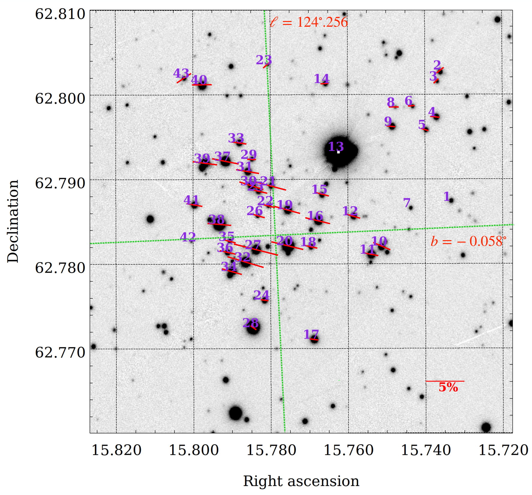
Most of the stars in the field have polarization angle oriented at a small angle to the Galactic plane while there are a few stars showing a larger deviation. The stars with larger deviation have slightly smaller degree of polarization (¡ 2.2 ) and maybe foreground objects. This is more clearly seen in the distribution of the polarization angle with the degree of polarization as shown in Figure 2.
On the basis of visual inspection, we have divided the stars into three groups separated by dotted lines:
- 1.
The first group contains four stars #2, #3, #23, and #43 having degree of polarization ranging between and polarization angle . The weighted mean polarization of this group is with dispersion of . The average polarization angle is showing a large deviation from the the galactic plane. This indicates that the stars in this group may be non-member/foreground stars.
- 2.
The second group consists of all the stars on the left side of the vertical dotted line marking (Figure 2). The stars present in this region have relatively smaller degree of polarization () with weighted average value of and dispersion of 0.12 but large spread in polarization angle (). The weighted average orientation of this group () is nearly parallel to the Galactic plane (having position angle of 91∘). These stars are distributed randomly in the outer regions of the core of the cluster (on the plane of the sky) and maybe foreground stars.
- 3.
The stars in the region with (Figure 2) forms the third group. The degree of polarization and polarization angle of stars in this group are ranging from and respectively. The average polarization is with a dispersion of . A large range in degree of polarization has been observed in many other clusters like Trumpler 27 (Feinstein et al. 2000), Hogg 22 and NGC 6204 (Martínez et al. 2004), NGC 5749 (Vergne et al. 2007), Berkeley 59 (Eswaraiah et al. 2012). The large spread in the degree of polarization could be due to several reasons which are discussed in section IV.2. The weighted average polarization angle of the stars in this group () is deviated from the Galactic plane ().
III.2 Distribution of polarization in the Stokes plane
Polarization can be used as an efficient tool in determining the cluster membership even if the colors of the member stars and the field stars are the same. The light from an intrinsically unpolarized star becomes partially polarized after passing through the asymmetrical but aligned dust grains present in the dust clouds of the ISM. The degree of polarization depends on the column density of aligned dust grains along the line of sight. The stars foreground to the dust cloud will be less polarized as compared to the stars behind the dust layers. Also, the polarization angle of the two may differ from each other depending upon the direction of the local magnetic field. It is expected that all the member stars are behind a common set of intervening clouds. Therefore, their polarization properties are expected to be similar while the field stars may have slightly different properties. The distribution of the stars in the Stokes -plane (with and ) is useful to distinguish the cluster members from the non-members. The members of the cluster are expected to group together in this plane while the field stars would show scattered distribution. However, intrinsic polarization, rotation of polarization angle and patchy extinction can also give rise to scattered distribution in the -plane.
The normalized () and () Stokes parameters are derived for all the observed stars and are plotted in Figure 3. The cross-section of dashed straight lines at = = 0 represents the dustless solar neighbourhood and the solid gray line corresponds to the Galactic plane (). The stars, on average, show a scattered distribution in the plane, which is expected for distant clusters because of the contamination by large number of foreground and/or background field stars. This has also been seen in Stock 6, NGC 1893 (Eswaraiah et al. 2011), and Berkeley 59 (Eswaraiah et al. 2012) clusters. It is difficult to identify the grouping of member stars in such cases. We draw box (black dashed box in Figure 3) with boundaries of mean and to elucidate the probable cluster members. All the stars within this box are considered as probable members and stars scattered away from the mean 1 box may have less membership probability. The , for groups 2 and 3 (as described in previous section III.1) are ranging from ; and ; respectively. To check the distribution of stars in these regions, we plotted the mean box corresponding to these two groups in blue (region 2) and red dotted lines (region 3) respectively in Figure 3. The blue dotted region is closer to the Sun and expected to consist of the foreground stars. While the member stars may be present in region 3. The stars outside the boxes are either field stars or having intrinsic component of polarization.
The plot is also helpful to study the evolution of interstellar environment from the Sun to the cluster. The two regions are separated by a gap suggesting two dust layers present between the Sun and the cluster. The first layer affects only the stars of region 2. The stars of region 3 exhibit a cumulative effect of both dust layers in their polarization.
More details of the membership and dust distribution are discussed together with distance, extinction and astrometric information in section IV.1.
IV Discussion
In the first subsection (IV.1) we redefine the cluster membership based on Gaia EDR3 astrometry. Subsection IV.2 discusses the polarization results of the 39 stars observed towards the core of Czernik 3 cluster in combination with different archival data. Dust distribution towards the Czernik 3 cluster is described in subsection IV.3. The general trend of polarization and its implications regarding the dust distribution over a large spatial range is in subsection IV.4.
IV.1 Membership from Gaia EDR3 data
The identification of member stars is important to determine the reliable cluster parameters like cluster radius, age and distance. In the past, photometry and polarization have been used to identify cluster members (Eswaraiah et al. 2011; Eswaraiah et al. 2012, etc.). Detailed discussion of cluster membership for Czernik 3, on the basis of polarization and photometry, is described in Appendix A. However, with the availability of the Gaia data it is found that astrometry is the best method to determine cluster membership. We have calculated the success rate of membership determination from polarization as compared to the astrometric method and it comes out to be 58.3% for Czernik 3 cluster. Hence, we mainly focus on the cluster membership based on astrometric method using parallax and proper motion information.
Figure 4 shows the proper motion (PM) versus degree of polarization (upper panel) and polarization angle (lower panel) of 39 stars listed in Table 3. There is a prominent clump around proper motion of mas/year. Two stars #23 and #28 are not shown in the figure because they have proper motion 10 mas/year and are non-members from polarization and photometric methods also (see Appendix A). According to the proper motion distribution, 23 stars - #4, #5, #6 #10, #12, #15, #16, #18, #19, #20, #21, #22, #25, #26, #27, #30, #32, #33, #35, #36, #39, #40, and #41 have higher membership probability than the other stars in the field showing scattered distribution in proper motion.
All the probable member stars (from Figure 4) except star #6 and #20 are also identified as members with probability (see column 4 of Table 4) using proper motion and parallax information of Gaia DR2 in UPMASK membership assignment code by Cantat-Gaudin et al. 2018. On the other hand Sharma et al. 2020 have selected the stars with high probability () of membership based on frequency distribution of member stars and field stars using Gaia DR2 proper motion information and have only 17 stars common with probable members from Figure 4 (see column 5 of Table 4). This has resulted in discrepancies of membership for individual stars between the two studies, as can be seen in the Table 4.
We have used the latest Gaia proper motion (PM) data (from Gaia EDR3) to redefine the membership probability. PMs, and are plotted as vector point diagrams (VPDs) in the top row of Figure 5 to see the distribution of cluster members and field stars towards the region of Czernik 3. The bottom row of this figure show the corresponding versus color magnitude diagrams (CMDs). The left panel in the CMD shows all the stars present within five arcmin radius around Czernik 3, while the middle and right panels show the possible cluster members and field stars, respectively. By visual inspection, we define the cluster center and radius in the VPD iteratively so as to reduce the contamination by the field stars while keeping a possible number of faint stars in the cluster sequence (middle panel of the CMD). A circle of 0.5 mas yr-1 around the center of the member stars distribution in the VPDs indicates our membership zone. We can see in the middle-bottom panel that the cluster’s main sequence is separated.
To identify the cluster members quantitatively, we have estimated the membership probabilities of the stars following the method given by Balaguer-Núnez et al. 1998.
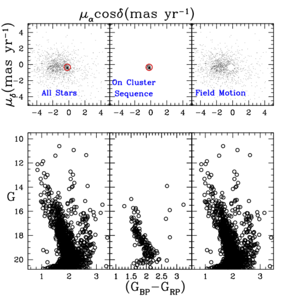
Many authors have previously used this method (Bellini et al. 2009; Sharma et al. 2020; Bisht et al. 2021; Sariya et al. 2021). Two distribution functions () and () for cluster and field stars are constructed for a particular ith star, which are given as follows:
| (7) | |||||
| (8) | |||||
where, (, ) are the PMs of star. The PM errors are represented by (, ). The cluster’s PM center, given by (, ) and (, ) represents the center of field PM values. The intrinsic PM dispersion for the cluster stars is denoted by , whereas and provide the intrinsic PM dispersion’s for the field populations. The correlation coefficient is calculated as:
| (9) |
In order to estimate probability of Czernik 3 star, we used only stars having PM errors better than 1 mas yr-1. We found a clear bunch of stars at = 0.22 mas yr-1, = 0.32 mas yr-1 and in the circular region with a radius of 0.5 mas yr-1 (Figure 5). We estimated dispersion () in PMs as 0.06 mas yr-1 by using cluster distance of 3.5 kpc (Sharma et al. 2020) and the radial velocity dispersion of 1 km for open star clusters (Girard et al. 1989). For field region stars, we have estimated (, ) = (0.95, 0.55) mas yr-1 and (, ) = (6.5, 4.4) mas yr-1.
In consideration of the normalized numbers of cluster and field stars as and respectively (i.e., ), the total distribution function can be estimated as
| (10) |
Finally, the membership probability for the star is given by
| (11) |
We obtain 72 cluster members in Czernik 3 cluster with membership probability higher than and mag.
The stellar density of the cluster region is affected by the presence of field region stars. So, we have calculated the effectiveness of membership determination for Czernik 3 using the formula given in eq. (12) (Shao & Zhao 1996):
| (12) |
where, is the total number of cluster members and indicates the probability of star of the cluster. The effectiveness value is obtained as 0.70 for Czernik 3. Shao & Zhao 1996 show that the effectiveness of membership determination of 43 open clusters ranges from 0.20 to 0.90 with the peak value of 0.55. Our estimated value is on the higher side but lies within the above limits. The mean distance of the Czernik 3 cluster is calculated using the distance information (Bailer-Jones et al. 2021) of the member stars present in the core (Sharma et al. 2020, ,) of the cluster. The average distance of the core members comes out to be kpc, which matches well with the distance determined by Sharma et al. 2020 using Gaia DR2 data. The membership probability of the observed stars is given in column 6 of Table 4.
A similar procedure is adopted to redefine the membership of the clusters IC 1805, NGC 654, Berkeley 59, NGC 457, and Alessi 1 using Gaia EDR3 data. From the revised cluster membership, the mean distance of each cluster is constrained to be 2.55 0.89, 2.89 0.72, 1.21 0.73, 2.87 0.72, and 0.72 0.17 kpc respectively. These values closely match with the average distance of the respective clusters in Cantat-Gaudin et al. 2018 (see Table 2).
| ID | Membership probability () | Membership probability () | Membership probability () | ||
|---|---|---|---|---|---|
| () | (∘) | (Cantat-Gaudin et al. 2018) | (Sharma et al. 2020) | (our study) | |
| 4 | 100 | - | 99.61 | ||
| 90 | - | 99.93 | |||
| 6 | - | 90 | 99.72 | ||
| 100 | 100 | 99.9 | |||
| 80 | 99 | 99.43 | |||
| 15 | 100 | 99 | 99.93 | ||
| 16 | 100 | 100 | 99.97 | ||
| 18 | 100 | 100 | 99.94 | ||
| 100 | 100 | 99.98 | |||
| 20 | - | 100 | 99.66 | ||
| 21 | 80 | - | 99.76 | ||
| 22 | 100 | 100 | 99.88 | ||
| 100 | 100 | 99.95 | |||
| 26 | 80 | - | 99.96 | ||
| 27 | 100 | 99 | 99.83 | ||
| 100 | 100 | 99.97 | |||
| 32 | 100 | 100 | 99.97 | ||
| 33 | 100 | - | 99.64 | ||
| 35 | 90 | 99 | 99.89 | ||
| 36 | 100 | 100 | 99.80 | ||
| 39 | 100 | 100 | 99.98 | ||
| 100 | - | 98.52 | |||
| 41 | 100 | 99 | 99.96 |
IV.2 On the variation of polarization over the Czernik 3 cluster
In this section we discuss the possible reasons for the large range in polarization observed over the stars of Czernik 3 cluster.
IV.2.1 Patchy dust distribution from WISE W4 image
Large dispersion in polarization values (Figure 2) could be due to the patchy distribution of dust along the line of sight towards Czernik 3 cluster, or due to the presence of dust within the cluster. This is further examined by analysing , WISE W4-band image33 3 https://irsa.ipac.caltech.edu/applications/wise/. Figure 6 shows the spatial distribution of dust (integrated emission along the line of sight) traced by WISE W4 band in field around Czernik 3. The red color contours represent the equal flux density points. Patchiness is well observed from the contour levels varying from 113.02 DN to 113.508 DN with interval of 0.054 DN. The uncertainty levels are DN. This implies that the dust is not distributed uniformly. It may be constant in small spatial areas but is highly variable across the face of the cluster. For example the central region of the cluster has higher flux density. Higher polarization in the same region is also observed, as seen by the length of the white colored polarization measurements centered at the star location. This is further discussed in section IV.2.4. Cyan and blue colored open circles in the figure denote the member and non-member stars. The patchy distribution has also been observed earlier in NGC 6823 open cluster embedded in the highly extincted region towards the inner Galaxy (Medhi et al. 2010).
Stars #4, #5, and #6 have low polarization , , and with large uncertainty in the polarization angle (, , and ). Even though these stars are present in box of group-2 (Figure 3), their proper motion data categorizes them as member stars with high membership probability (). The low value of the polarization can be explained by the lesser dust column density traversed by the light coming from these stars, as seen by the contour level being DN.
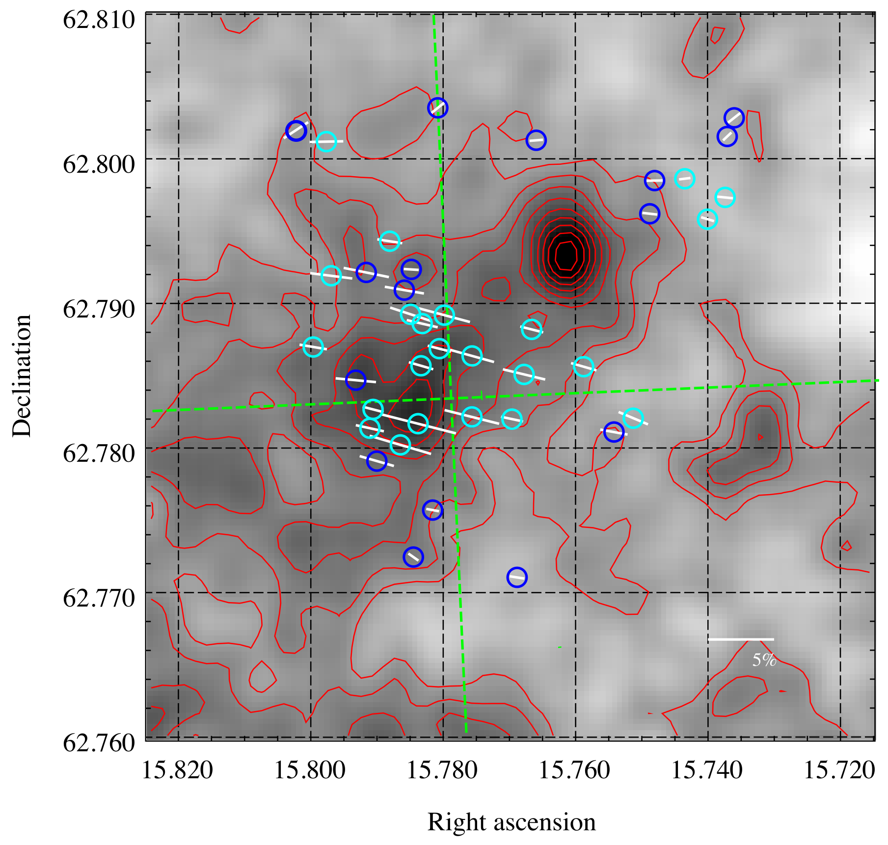
On the contrary, the core region stars #21, #27 and #32 show large degree of polarization (, and ) because of higher dust density at central region as compared to peripheral region. The proper motion and polarization angle (, and ) of these stars are similar to the member stars but lying outside region 3 in -plot (Figure 3), which may be due to non-uniform dust distribution.
IV.2.2 Polarization efficiency
The degree of polarization produced for a given amount of extinction is referred to as polarization efficiency of the intervening dust grains. It is known that the polarization efficiency of the ISM is non-uniform. This can be seen from large scatter in Figure 7, which shows the relation between color excess and i-band polarization for the stars observed by us along the line of sight of Czernik 3 cluster. The efficiency depends on the degree of alignment of the dust grains with the magnetic field and also on the amount of depolarization due to radiation traversing more than one cloud with different magnetic field directions. The empirical upper limit (Hiltner 1956) for maximum polarization efficiency of diffuse ISM at visual wavelengths assuming (Seaton 1979) is given by
| (13) |
The polarization efficiency in Sloan i-band () is determined using Serkowski’s law for interstellar polarization by assuming maximum polarization at average wavelength with K= 1.15 (Whittet 2003) and is given by eq. (14) (dashed line in Figure 7).
| (14) |
However, the varies from star to star and has a typical range of (Whittet 2003). Many studies (Wilking et al. 1980; Wilking et al. 1982; Clayton et al. 1995; Martin et al. 1999, e.g,) have shown that the and K are linearly correlated by the Wilking law:
| (15) |
Where, the constants and are given by m-1 and in visible to near infrared (VIR) wavelength regime () (Whittet 1992). In order to explore the effect of polarization efficiency in the Sloan i-band, we have considered and eq. (15) for the K values, in the Serkowski law of interstellar polarization. The resulting broad range of empirical relations cover an area demarcated by light grey colored region in the Figure 7.
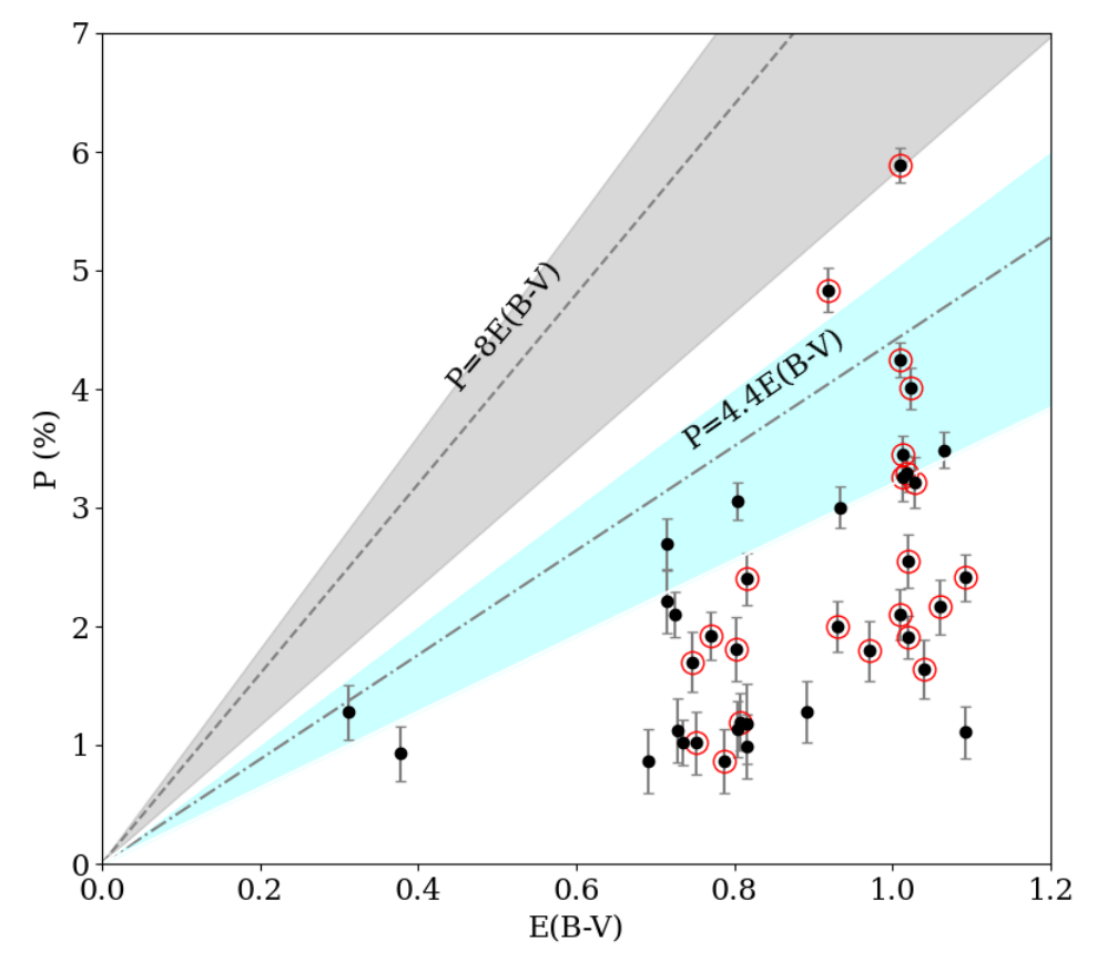
The polarization efficiency of the diffuse ISM, in general, follows the mean relation (Serkowski et al. 1975). The corresponding Sloan i-filter polarization as a function of E(B-V) is calculated to be and it is shown by dash-dotted line (with = 0.55 m, K=1.15) and cyan shaded region (corresponding to the range in ) in the same figure. The observed polarization efficiency towards the cluster is less than the empirical upper limit defined by the light grey shaded region described earlier. A few stars (member as well as non-member) are showing efficiency more than the general diffuse ISM considering varying as seen from their appearance above the lower limit of the cyan shaded region. Out of these, two stars (#27 and #32) are lying above the maximum of the cyan shaded region, indicating different polarization behaviour as compared to the diffuse ISM. These two stars are near the center of the cluster, where there is an excess of dust (see the discussion in section IV.2.1). It is also possible that they are both intrinsically polarized (see the discussion in Section IV.2.3) for example, #27 is an evolved (probable AGB) star where one may expect intrinsic polarization due to an asymmetric dust shell.
IV.2.3 Intrinsic polarization
Stars having circumstellar dust, can show intrinsic polarization which may be different from the interstellar polarization. Young stellar objects and evolved stars are the possible candidates to show intrinsic polarization. Recently, Marton et al. 2019 classified stars into four categories, i.e., extincted main sequence stars, evolved stars, extra-galactic sources and, young stellar objects using machine learning techniques by considering Gaia DR2 and ALLWISE data. We have found entries for 10 of our observed stars in this catalog44 4 https://vizier.u-strasbg.fr/viz-bin/VizieR?-source=II/360. The probabilities of each category with their errors are listed in Table 5. We have opted to use their probability columns which do not consider the W3 and W4 band fluxes since the ‘R’ parameter (first column in the Table 5), which represents the probability for W3 and W4 detections to be real, is less than 75% for all 10 stars. From the Table 5, 7 stars (#3, #10, #17, #19, #23, #28 and #40) are highly probable YSO candidates, out of which #10 #19 and #40 (with underlined ID) are cluster members and stars #27 and #38 have high probability of being evolved stars.
| ID | R | SE | SEG | SMS | SY | ||||
|---|---|---|---|---|---|---|---|---|---|
| 3 | 0.378 | 0.0784 | 0.04382 | 0.1492 | 0.06497 | 2.0E-4 | 6.3E-4 | 0.7722 | 0.09265 |
| 10 | 0.448 | 0.0768 | 0.03213 | 0.2426 | 0.11013 | 0.0236 | 0.06561 | 0.657 | 0.10294 |
| 17 | 0.438 | 0.0572 | 0.0351 | 0.0664 | 0.04666 | 0.0094 | 0.01276 | 0.867 | 0.07939 |
| 19 | 0.278 | 0.0704 | 0.0182 | 0.0848 | 0.02443 | 0.0048 | 0.00492 | 0.84 | 0.03307 |
| 23 | 0.43 | 0.1234 | 0.06507 | 0.0482 | 0.01853 | 0.0012 | 0.0038 | 0.8272 | 0.07272 |
| 27 | 0.646 | 0.6674 | 0.08052 | 0.0076 | 0.0044 | 0.0112 | 0.01237 | 0.3138 | 0.07726 |
| 28 | 0.348 | 0.2232 | 0.03774 | 0.0172 | 0.01084 | 0.0336 | 0.01622 | 0.726 | 0.04233 |
| 38 | 0.65 | 0.9118 | 0.04445 | 0.0224 | 0.02948 | 0.0084 | 0.00858 | 0.0574 | 0.01718 |
| 40 | 0.45 | 0.101 | 0.03923 | 0.0576 | 0.02965 | 0.0058 | 0.00577 | 0.8356 | 0.04639 |
YSO candidates can also be identified using reddening parameter Q. The stars are considered as a candidate young stellar object if the reddening-free parameter Q becomes less than (Buckner & Froebrich 2013). The Q value can be estimated for a star using the VVV photometric magnitude relationship given by
| (16) |
We used the 2MASS photometric values for our stars transformed to VVV using transformation equations of 1.5 version of CASU photometry (González-Fernández et al. 2018) to obtain the Q parameter. We find 5 candidate YSOs (#5, #12, #24, #25, #30) using the above relation of which #5, #12, #25, and #30 are cluster members.
Thus, in total 7 member YSOs candidates have been detected in Czernik 3. The intrinsic polarization due to the circumstellar disk can be a cause of scattered position in the -plane for some of these stars. These stars are marked with asterisk and double asterisk in the ID column of the Table 4.
IV.2.4 Spatial variation of polarization
First two panels of Figure 8 show the variation of degree of polarization and polarization angle with angular distance from the center of the cluster. The angular distance of a star having equatorial co-ordinates () from the center of the cluster () is given by the eq. (17).
| (17) |
The third panel represents the WISE W4 flux (in Jy) as a function of angular distance. This flux is obtained by using aperture photometry on the position of the stars using a fixed aperture. A decrease is seen in the WISE flux as well as degree of polarization radially outwards. The polarization angle exhibits a very small dispersion in the core region (radius of (Sharma et al. 2020) - marked by dashed line) while the dispersion increases in the outer directions. This suggests that the dust is more concentrated towards the center and the density decreases with the radial distance from the cluster center. The small dispersion in polarization angle with increased degree of polarization also indicates that the dust in the cluster is oriented in the same direction as the dust in the interstellar medium. This implies that the dust in the cluster seems to be relaxed with reference to the interstellar magnetic field i.e., the dust grains in the cluster are magnetically aligned with the large-scale magnetic field at the location of the cluster.
IV.3 Dust distribution towards Czernik 3
Polarization value shows a change when light from the stars encounters dust layers at different distances in the line of sight. The degree of polarization increases after passing through each dust layer if the orientation of the magnetic field is uniform in all dust clouds and becomes depolarized if the orientation of the magnetic field are different. The number of such changes in the degree of polarization as well as in extinction corresponds to the number of dust layers. Thus, the distribution of dust along the line of sight can be studied by analysing polarization with distance. In order to quantify the distances of the dust clouds, we have used distance information () of individual stars from Bailer-Jones et al. 2021. One star, #20, does not have the value. Consequently, we have used the (distance estimated from EDR3 parallax using Geometric prior only) value for that source. Figure 9 shows the variation of polarization, position angle, and E(B-V) with distance (). The E(B-V) values are taken from Green et al. 2019 (Green 2018, calculated using a python based script presented by). The cluster members are marked as red open circles. Middle panel of Figure 9 reveals a significant change in the polarization angle between star #43 and #34. This indicates the presence of a dust layer at a distance 1800 pc (upper limit). We also note that there is an increase (top panel) in the degree of polarization just beyond pc. Due to the lack of polarization data for stars below 2000 pc, it is difficult to constrain the distance of the foreground dust cloud. However, the E(B-V) values shows a jump at a distance 1200 pc (see bottom panel of Figure 9). This could be because of the presence of LDN1306, a Lynd’s dark cloud (Lynds 1962). The cloud has an angular extent of (Dutra & Bica 2002) and it is present south-east to the cluster with angular separation of . The reported percentile distance to the cloud is pc (Zucker et al. 2020), which is consistent with the location of the observed change in the degree of polarization as well as in E(B-V) close to pc.
and percentile reddening (E(B-V)) as a function of distance.
Stars beyond 2000 pc have large uncertainties (see Figures 14 (a) and (b), along with Figure 9) associated with the distance (). However, E(B-V) value shows a systematic change with distance, indicating another dust layer around 3450 pc. The spread in distance of the member stars (shown as red open circles in Figure 9) is the result of large fractional parallax errors of these distant sources. The presence of a dust layer around 3450 pc nearly coinciding with the average distance to the cluster ( pc) indicates the following possibilities:
- 1.
the cluster may be embedded in the dust layer
- 2.
the cluster is passing through a dense region of the galactic plane and coincidentally has a similar distance as that of a cloud near that location
- 3.
the dust layer is present just before the cluster.
To confirm the presence of the second dust layer, we consider the fact that dust and HI are correlated in the diffuse ISM (Bohlin et al. 1978, e.g.,). Therefore, we use kinematic information of HI line emission spectra from HI4PI survey (HI4PI Collaboration et al. 2016) to infer the distribution of atomic gas along the line of sight in the selected region. The spectrum (blue line in Figure 15) reveals the existence of four well separated velocity peaks (-114.7, -100.4, -43.8, -13.0 K ms-1) and implies the neutral ISM mass is distributed in at least 4 spatially distinct components along the line of sight. The calculated kinematic distance of corresponding peak is given in Table 6 (detailed information is given in Appendix C). Clouds with peak velocity -114.7 km s-1 and -100 km s-1 are in the background of the cluster (distance 6 kpc). Thus, they will not contribute to the observed polarization. The main contribution comes from the clouds having distance of kpc and which is consistent with the color excess and polarization jumps observed in the Figure 9. The same two clouds with radial velocity of km s-1, km s-1 are also seen in the molecular data (orange line in Figure 15), i.e., spectral information of 12CO from Dame et al. 2001. This confirms the presence of at-least two clouds along our line of sight.
In addition, the variation in E(B-V) and degree of polarization of the member stars with distance (Figure 9) also suggests patchy extinction present towards the Czernik 3 cluster.
IV.4 General trend of dust distribution: a signature of Inter-arm region
In this section, we study the global properties of dust distribution that can be derived by combining the polarization data of Czernik 3, one of the most distant clusters with polarization data, and other clusters present within 15∘ region around it (see Table 2) along with the Heiles 2000 stars (Figure 10).
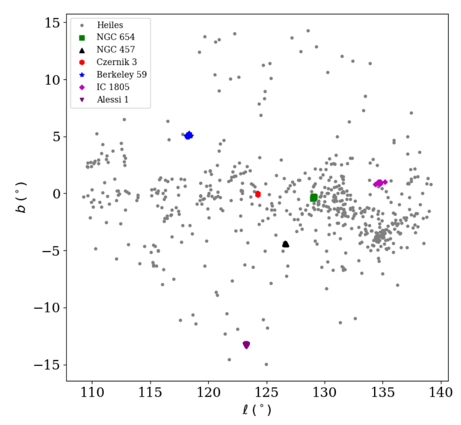
The polarization measurements of these clusters were converted to equivalent values in the Sloan - i band by utilizing the respective and values in the Serkowski law for wavelength dependence of polarization. The degree of polarization of all the available clusters in sloan i-band, along this direction is plotted as a function of distance (, pc) in Figure 11.
The polarization of stars within of Czernik 3 from Heiles 2000 is also added in gray color. It is seen that the degree of polarization gradually increases with distance as expected from the uniform dust distribution close to the solar neighbourhood (in the local arm) but shows a sudden increase due to a dust patch at 700 pc (Eswaraiah et al. 2012). There is a drop in the number of stars between 1-2 kpc in all the cluster fields as well as the field stars from the Heiles catalog and there is no systematic change in polarization in this region. The polarization angle also remains consistent in the two regions ( 1kpc & 2kpc). This peculiar decrease in number of stars and no observed systematic change in polarization indicates that this region may contain minimal dust to affect the polarization of the background stars. This decrease in the number of stars with polarization measurement is not due to sample incompleteness. Rather, we note that the overall stellar number density (detection in the 2MASS bands with quality flag ‘AAA’) also shows a significant drop between 1 and 2 Kpc. The decline in stellar density as well as dust density (from polarization data) suggests that the 1-2 Kpc region could be the inter-arm region between the local arm (below 1 kpc) and the Perseus arm (Xu et al. 2006, 2kpc, ).
The variation of average degree of polarization of each cluster with the mean distance of the member stars (membership probability ) with polarization measurement is depicted in Figure 12.

This figure shows a decrease in mean polarization of the cluster with distance.
We note that Alessi 1 is a high latitude cluster (see Figure 10), suffering lesser dust extinction as compared to other clusters, hence showing exceptionally low degree of polarization in comparison to the others. On the other hand Berkeley 59 is a young cluster having intra-cluster dust due to which many cluster members have intrinsic (non-interstellar) polarization up to 2% (Eswaraiah et al. 2012). The other clusters considered here, are relatively older. With these caveats in mind, we still see an overall decrease in the degree of polarization with distance (Figure 12), which could be due to decrease in polarization efficiency with increasing path length.
V Conclusions
In this work, we presented the linear polarization study towards a distant open cluster, Czernik 3 and 15∘ region around it, with the aim to estimate the dust distribution on different spatial scales. We also redefined the membership of Czernik 3 as well as the other nearby clusters, having polarization information, considered in this work. The polarimetric observations of Czernik 3 were carried out using the EMPOL instrument at the 1.2 m telescope at Mount Abu. A total of 42 stars are observed towards the core region of the cluster in Sloan i-band. We have arrived at the following conclusions from our study:
- 1.
From the observed changes in the degree of polarization and extinction, we infer the presence of two dust clouds along the line of sight towards Czernik 3 cluster, at distances of kpc and kpc. The first cloud corresponds to the Lynds dark nebula LDN 1306.
- 2.
The large range in the observed polarization () of Czernik 3 stars may result from a non-uniform polarization efficiency. It could also arise from the non-uniform/patchy distribution of dust towards the cluster. We observed more dust density in the core of the cluster as compared to the peripheral regions.
- 3.
The cluster membership of Czernik 3 as well as other nearby clusters is redefined using the astrometric and photometric data from the latest Gaia EDR3. The distance to the Czernik 3 cluster is well constrained using member stars present in the core and it comes out to be kpc.
- 4.
The polarization efficiency for most of the observed stars towards Czernik 3 is less than the upper limit of the empirical relation for ISM polarization. Two stars with exceptionally high polarization are closer to the center of the cluster indicating different polarization behaviour as compared to the general diffuse ISM. They may also be intrinsically polarized.
- 5.
For the clusters studied here, we find that the average polarization of the cluster decreases with distance to the cluster, indicating a decrease in polarization efficiency with increasing path length.
- 6.
There is a decrease in dust as well as stellar density in the distance range of 1 to 2 kpc in a 15∘ wide region around Czernik 3. This is speculated to be the inter-arm region between the local arm and the Perseus arm.
VI Acknowledgement
We thank the referee, Dr Enrique Lopez-Rodriguez, for his careful evaluation of the manuscript and the insightful comments which helped to improve the paper. We thank the local staff at Mount Abu Observatory, PRL for their help during observations. We would also like to thank Prof U C Joshi, Prof K S Baliyan and our colleagues in the Astronomy and Astrophysics division, PRL for useful discussions. Work at Physical Research Laboratory is supported by the Department of Space, Govt. of India. A part of this work has made use of data from the European Space Agency (ESA) mission Gaia55 5 https://www.cosmos.esa.int/web/gaia, processed by the Gaia Data Processing and Analysis Consortium (DPAC66 6 https://www.cosmos.esa.int/web/gaia/dpac/consortium). Funding for the DPAC is provided by national institutions, in particular, the institutions participating in the Gaia Multilateral Agreement. This research made use of Astropy,77 7 http://www.astropy.org a community-developed core Python package for Astronomy (Astropy Collaboration et al. 2013; Astropy Collaboration et al. 2018). We have also used the VizieR catalogue access tool, CDS, Strasbourg, France.
Appendix A Cluster membership through photometric and polarimetric approach
It is expected that all the member stars are behind the same dust clouds, thus the colour-excess of the member stars should be comparable to the mean colour-excess of the cluster. In comparison, the field stars suffer varying extinction based on whether they are present foreground or background to the cluster. Medhi & Tamura 2013 have shown that the TCD together with the polarization can be used to distinguish the cluster members from the field stars.
We now consider the stars in the plane of Figure 3 in the context of their PanSTARRS magnitudes and colours. The PanSTARRS apparent color-magnitude diagram and TCD for a region around the cluster is shown in Figure 13 (a) and (b). The ID of the stars listed in the Table 3 are labeled in these two figures.
The group-1 stars(#2, #3, #23, and #43) of Figure 2 have polarization angle larger than that of the Galactic plane and lie outside the mean box on plane (Figure 3) with range of and . Stars #3 and #23 show more reddening (see Figure 13 (a) and (b)) than the bulk of the stars. Hence, these two stars are not member stars according to both approaches (photometric and polarimetric). Though the color of stars #2 and #43 are similar to the member stars, their location in the plot and their position angle values indicate deviation from polarization angle of member stars. Hence, these stars are also considered as non-members.
Star #28 have q -0.5 (outside mean box in Figure 3) just like #2, #3 and #23 and have large errors associated with their polarization values. It has a low value of polarization - and polarization angle which is quite different from the rest of the stars. This indicates that #28 could be a foreground star, which is consistent with relatively bluer color r-i = 0.31 and a Gaia EDR3 distance of 409 pc.
Stars #27 and #38 are reddened in colour (see Figure 13 (a) and (b)). Star #27 shows highest polarization () in our data set while the polarization angle () is similar to the member stars (group 3 stars). It may be a member star having some intrinsic component of polarization. On the other hand, Star #38 is outside the mean boundary of group 3 in plane (see Figure 3) and shows a deviation in polarization angle () from mean polarization angle of group 3 stars. It is highly probable that this star may also have intrinsic polarization. Discussion about its cluster membership is deferred to the Section IV.1. The rest of the distribution in the plane is scattered, however, the region 3 of Figure 3 contains the most probable cluster members.
Considering only photo-polarimetric approach, the contribution to the cluster membership, by the field stars, can be overestimated if there is a common dust layer foreground to the field stars and the cluster members. Hence, polarization alone cannot be used to estimate the membership probability of distant open clusters.
Appendix B Variation of polarization with distance
The variation of degree of polarization and polarization angles as a function of distance () along with their corresponding error-bars are displayed in Figure 14 (a) and (b) respectively. Detailed discussion is available in section IV.3
Appendix C Distance calculation of H1 and 12CO clouds
The spectral information of 21-cm neutral hydrogen line (HI) within region of Czernik 3 cluster centered at is taken from the HI4PI survey (angular resolution: 16′.2) and is shown as blue curve in Figure 15. The HI peaks show the presence of multiple clouds in the line of sight with peak velocity of km s-1, km s-1, km s-1, km s-1, and km s-1. There could be two more clouds with peak velocities of and km s-1. The orange curve in the Figure 15 represents the spectral information of 12CO (angular resolution: ) within the region around the center of the cluster and indicates three clouds along the line of sight with peak velocity closer to the first three HI clouds.
The kinematic distance of the HI and 12CO clouds are calculated from the web interface88 8 http://bessel.vlbi-astrometry.org/revised_kd_2014? corresponding to the source code provided by Reid et al. 2009. We have used the Galactic parameters : km s-1, kpc, km s-1 kpc-1, km s-1, km s-1, km s-1, km s-1, km s-1 following A5 model of Reid et al. 2014. The corresponding distances are tabulated in Table 6.
Three clouds are seen in common (at similar velocities) in both HI as well as 12CO. The neutral hydrogen, HI traces the diffuse medium while 12CO traces the outer regions of dense molecular clouds. Therefore, we consider clouds having 12CO data coinciding with HI radial velocity peaks around km s-1 and km s-1.
| Line of sight velocity (Km s-1) | Kinematic distance (kpc) |
|---|---|
| -114.7 | |
| -100.4 | |
| -67.0 | |
| -55.3 | |
| -43.7 | |
| -13.0 |
References
- Astropy Collaboration et al. (2013) Astropy Collaboration, Robitaille, T. P., Tollerud, E. J., et al. 2013, A&A, 558, A33, doi: 10.1051/0004-6361/201322068
- Astropy Collaboration et al. (2018) Astropy Collaboration, Price-Whelan, A. M., Sipőcz, B. M., et al. 2018, AJ, 156, 123, doi: 10.3847/1538-3881/aabc4f
- Axon & Ellis (1976) Axon, D. J., & Ellis, R. S. 1976, MNRAS, 177, 499, doi: 10.1093/mnras/177.3.499
- Bailer-Jones et al. (2021) Bailer-Jones, C. A. L., Rybizki, J., Fouesneau, M., Demleitner, M., & Andrae, R. 2021, AJ, 161, 147, doi: 10.3847/1538-3881/abd806
- Balaguer-Núnez et al. (1998) Balaguer-Núnez, L., Tian, K. P., & Zhao, J. L. 1998, A&AS, 133, 387, doi: 10.1051/aas:1998324
- Bellini et al. (2009) Bellini, A., Piotto, G., Bedin, L. R., et al. 2009, A&A, 493, 959, doi: 10.1051/0004-6361:200810880
- Berdyugin et al. (2014) Berdyugin, A., Piirola, V., & Teerikorpi, P. 2014, A&A, 561, A24, doi: 10.1051/0004-6361/201322604
- Bertin & Arnouts (1996) Bertin, E., & Arnouts, S. 1996, A&AS, 117, 393, doi: 10.1051/aas:1996164
- Bisht et al. (2017) Bisht, D., Yadav, R. K. S., & Durgapal, A. K. 2017, New A, 52, 55, doi: 10.1016/j.newast.2016.10.009
- Bisht et al. (2021) Bisht, D., Zhu, Q., Yadav, R., et al. 2021, MNRAS, 503, 5929B, doi: 10.1093/mnras/stab691
- Boch et al. (2012) Boch, T., Pineau, F., & Derriere, S. 2012, in Astronomical Society of the Pacific Conference Series, Vol. 461, Astronomical Data Analysis Software and Systems XXI, ed. P. Ballester, D. Egret, & N. P. F. Lorente, 291
- Bohlin et al. (1978) Bohlin, R. C., Savage, B. D., & Drake, J. F. 1978, ApJ, 224, 132, doi: 10.1086/156357
- Bradley et al. (2020) Bradley, L., Sipőcz, B., Robitaille, T., et al. 2020, astropy/photutils: 1.0.0, 1.0.0, Zenodo, doi: 10.5281/zenodo.4044744
- Buckner & Froebrich (2013) Buckner, A. S. M., & Froebrich, D. 2013, MNRAS, 436, 1465, doi: 10.1093/mnras/stt1665
- Cantat-Gaudin et al. (2018) Cantat-Gaudin, T., Jordi, C., Vallenari, A., et al. 2018, A&A, 618, A93, doi: 10.1051/0004-6361/201833476
- Castro-Ginard et al. (2021) Castro-Ginard, A., McMillan, P. J., Luri, X., et al. 2021, A&A, 652, A162, doi: 10.1051/0004-6361/202039751
- Chambers et al. (2016) Chambers, K. C., Magnier, E. A., Metcalfe, N., et al. 2016, arXiv e-prints, arXiv:1612.05560. https://arxiv.org/abs/1612.05560
- Clayton et al. (1995) Clayton, G. C., Wolff, M. J., Allen, R. G., & Lupie, O. L. 1995, ApJ, 445, 947, doi: 10.1086/175754
- Clayton et al. (2003) Clayton, G. C., Wolff, M. J., Sofia, U. J., Gordon, K. D., & Misselt, K. A. 2003, ApJ, 588, 871, doi: 10.1086/374316
- Clemens et al. (2020) Clemens, D. P., Cashman, L. R., Cerny, C., et al. 2020, ApJS, 249, 23, doi: 10.3847/1538-4365/ab9f30
- Cutri et al. (2003) Cutri, R. M., Skrutskie, M. F., van Dyk, S., et al. 2003, 2MASS All Sky Catalog of point sources.
- Dame et al. (2001) Dame, T. M., Hartmann, D., & Thaddeus, P. 2001, ApJ, 547, 792, doi: 10.1086/318388
- Dias et al. (2002) Dias, W. S., Alessi, B. S., Moitinho, A., & Lépine, J. R. D. 2002, A&A, 389, 871, doi: 10.1051/0004-6361:20020668
- Dutra & Bica (2002) Dutra, C. M., & Bica, E. 2002, A&A, 383, 631, doi: 10.1051/0004-6361:20011761
- Eswaraiah et al. (2012) Eswaraiah, C., Pandey, A. K., Maheswar, G., et al. 2012, MNRAS, 419, 2587, doi: 10.1111/j.1365-2966.2011.19908.x
- Eswaraiah et al. (2011) —. 2011, MNRAS, 411, 1418, doi: 10.1111/j.1365-2966.2010.17780.x
- Fabricius et al. (2021) Fabricius, C., Luri, X., Arenou, F., et al. 2021, A&A, 649, A5, doi: 10.1051/0004-6361/202039834
- Feinstein et al. (2000) Feinstein, C., Baume, G., Vazquez, R., Niemela, V., & Cerruti, M. A. 2000, AJ, 120, 1906, doi: 10.1086/301562
- Gaia Collaboration et al. (2021) Gaia Collaboration, Brown, A. G. A., Vallenari, A., et al. 2021, A&A, 649, A1, doi: 10.1051/0004-6361/202039657
- Ganesh et al. (2020) Ganesh, S., Rai, A., Aravind, K., et al. 2020, in Society of Photo-Optical Instrumentation Engineers (SPIE) Conference Series, Vol. 11447, Society of Photo-Optical Instrumentation Engineers (SPIE) Conference Series, 114479E, doi: 10.1117/12.2560949
- Girard et al. (1989) Girard, T. M., Grundy, W. M., Lopez, C. E., & van Altena, W. F. 1989, AJ, 98, 227G, doi: 10.1086/115139
- González-Fernández et al. (2018) González-Fernández, C., Hodgkin, S. T., Irwin, M. J., et al. 2018, MNRAS, 474, 5459, doi: 10.1093/mnras/stx3073
- Goodman et al. (1990) Goodman, A. A., Bastien, P., Myers, P. C., & Menard, F. 1990, ApJ, 359, 363, doi: 10.1086/169070
- Green (2018) Green, G. M. 2018, The Journal of Open Source Software, 3, 695, doi: 10.21105/joss.00695
- Green et al. (2019) Green, G. M., Schlafly, E., Zucker, C., Speagle, J. S., & Finkbeiner, D. 2019, ApJ, 887, 93, doi: 10.3847/1538-4357/ab5362
- Hao et al. (2021) Hao, C. J., Xu, Y., Hou, L. G., et al. 2021, A&A, 652, A102, doi: 10.1051/0004-6361/202140608
- Heiles (2000) Heiles, C. 2000, AJ, 119, 923, doi: 10.1086/301236
- HI4PI Collaboration et al. (2016) HI4PI Collaboration, Ben Bekhti, N., Flöer, L., et al. 2016, A&A, 594, A116, doi: 10.1051/0004-6361/201629178
- Hiltner (1956) Hiltner, W. A. 1956, ApJS, 2, 389, doi: 10.1086/190029
- Joshi et al. (2016) Joshi, Y. C., Dambis, A. K., Pandey, A. K., & Joshi, S. 2016, A&A, 593, A116, doi: 10.1051/0004-6361/201628944
- Kharchenko et al. (2013) Kharchenko, N. V., Piskunov, A. E., Schilbach, E., Röser, S., & Scholz, R. D. 2013, A&A, 558, A53, doi: 10.1051/0004-6361/201322302
- Kharchenko et al. (2016) —. 2016, A&A, 585, A101, doi: 10.1051/0004-6361/201527292
- Kim & Martin (1994) Kim, S.-H., & Martin, P. G. 1994, ApJ, 431, 783, doi: 10.1086/174529
- Kim & Martin (1995) —. 1995, ApJ, 444, 293, doi: 10.1086/175604
- Lallement et al. (2019) Lallement, R., Babusiaux, C., Vergely, J. L., et al. 2019, A&A, 625, A135, doi: 10.1051/0004-6361/201834695
- Lynds (1962) Lynds, B. T. 1962, ApJS, 7, 1, doi: 10.1086/190072
- Martin et al. (1999) Martin, P. G., Clayton, G. C., & Wolff, M. J. 1999, ApJ, 510, 905, doi: 10.1086/306613
- Martínez et al. (2004) Martínez, R., Vergne, M. M., & Feinstein, C. 2004, A&A, 419, 965, doi: 10.1051/0004-6361:20035635
- Marton et al. (2019) Marton, G., Ábrahám, P., Szegedi-Elek, E., et al. 2019, MNRAS, 487, 2522, doi: 10.1093/mnras/stz1301
- Mathewson & Ford (1971) Mathewson, D. S., & Ford, V. L. 1971, MNRAS, 153, 525, doi: 10.1093/mnras/153.4.525
- Mathis (1986) Mathis, J. S. 1986, ApJ, 308, 281, doi: 10.1086/164499
- Medhi et al. (2007) Medhi, B. J., Maheswar, G., Brijesh, K., et al. 2007, MNRAS, 378, 881, doi: 10.1111/j.1365-2966.2007.11767.x
- Medhi et al. (2008) Medhi, B. J., Maheswar, G., Pandey, J. C., Kumar, T. S., & Sagar, R. 2008, MNRAS, 388, 105, doi: 10.1111/j.1365-2966.2008.13405.x
- Medhi et al. (2010) Medhi, B. J., Maheswar G., Pandey, J. C., Tamura, M., & Sagar, R. 2010, MNRAS, 403, 1577, doi: 10.1111/j.1365-2966.2010.16221.x
- Medhi & Tamura (2013) Medhi, B. J., & Tamura, M. 2013, MNRAS, 430, 1334, doi: 10.1093/mnras/sts714
- Mink (2011) Mink, J. 2011, WCSTools: Image Astrometry Toolkit. http://ascl.net/1109.015
- NASA/IPAC Infrared Science Archive (2020) NASA/IPAC Infrared Science Archive. 2020, WISE All-Sky 4-band Atlas Coadded Images, IPAC, doi: 10.26131/IRSA151
- Pancharatnam (1955) Pancharatnam, S. 1955, Proceedings of the Indian Academy of Sciences - Section A, 41, 137, doi: 10.1007/bf03047098
- Papoular (2018) Papoular, R. 2018, MNRAS, 479, 1685, doi: 10.1093/mnras/sty1530
- Reid et al. (2009) Reid, M. J., Menten, K. M., Zheng, X. W., et al. 2009, ApJ, 700, 137, doi: 10.1088/0004-637X/700/1/137
- Reid et al. (2014) Reid, M. J., Menten, K. M., Brunthaler, A., et al. 2014, ApJ, 783, 130, doi: 10.1088/0004-637X/783/2/130
- Sariya et al. (2021) Sariya, D., Jiang, I.-G., Bisht, D., Yadav, R., & Rangwal, G. 2021, AJ, 161, 102S, doi: 10.3847/1538-3881/abd31f
- Schmidt et al. (1992) Schmidt, G. D., Elston, R., & Lupie, O. L. 1992, AJ, 104, 1563, doi: 10.1086/116341
- Seaton (1979) Seaton, M. J. 1979, MNRAS, 187, 73, doi: 10.1093/mnras/187.1.73P
- Serkowski et al. (1975) Serkowski, K., Mathewson, D. S., & Ford, V. L. 1975, ApJ, 196, 261, doi: 10.1086/153410
- Shao & Zhao (1996) Shao, Z., & Zhao, J. 1996, Acta Astron. Sinica, 37, 377S
- Sharma et al. (2020) Sharma, S., Ghosh, A., Ojha, D. K., et al. 2020, MNRAS, 498, 2309, doi: 10.1093/mnras/staa2412
- Singh & Pandey (2020) Singh, S., & Pandey, J. C. 2020, AJ, 160, 256, doi: 10.3847/1538-3881/abba29
- Singh et al. (2020) Singh, S., Pandey, J. C., Yadav, R. K. S., & Medhi, B. J. 2020, AJ, 159, 99, doi: 10.3847/1538-3881/ab6608
- Topasna et al. (2017) Topasna, G. A., Daman, E. A., & Kaltcheva, N. T. 2017, PASP, 129, 104201, doi: 10.1088/1538-3873/aa7f6c
- Topasna et al. (2018) Topasna, G. A., Kaltcheva, N. T., & Paunzen, E. 2018, A&A, 615, A166, doi: 10.1051/0004-6361/201731903
- Vergne et al. (2007) Vergne, M. M., Feinstein, C., & Martínez, R. 2007, A&A, 462, 621, doi: 10.1051/0004-6361:20042124
- Voshchinnikov & Das (2008) Voshchinnikov, N. V., & Das, H. K. 2008, J. Quant. Spec. Radiat. Transf., 109, 1527, doi: 10.1016/j.jqsrt.2008.01.003
- Whittet (2003) Whittet, D. 2003, Dust in the galactic environment
- Whittet (1992) Whittet, D. C. B. 1992, Dust in the galactic environment
- Wilking et al. (1980) Wilking, B. A., Lebofsky, M. J., Martin, P. G., Rieke, G. H., & Kemp, J. C. 1980, ApJ, 235, 905, doi: 10.1086/157694
- Wilking et al. (1982) Wilking, B. A., Lebofsky, M. J., & Rieke, G. H. 1982, AJ, 87, 695, doi: 10.1086/113147
- Xu et al. (2006) Xu, Y., Reid, M. J., Zheng, X. W., & Menten, K. M. 2006, Science, 311, 54, doi: 10.1126/science.1120914
- Zacharias et al. (2013) Zacharias, N., Finch, C. T., Girard, T. M., et al. 2013, AJ, 145, 44, doi: 10.1088/0004-6256/145/2/44
- Zucker et al. (2020) Zucker, C., Speagle, J. S., Schlafly, E. F., et al. 2020, A&A, 633, A51, doi: 10.1051/0004-6361/201936145