MixMAE: Mixed and Masked Autoencoder for Efficient Pretraining of Hierarchical Vision Transformers

Jihao Liu Affiliation: CUHK MMLab Affiliation: SenseTime Research Xin Huang Affiliation: SenseTime Research Jinliang Zheng Affiliation: SenseTime Research Yu Liu Affiliation: SenseTime Research Hongsheng Li Affiliation: CUHK MMLab Affiliation: CPII under InnoHK

Abstract

In this paper, we propose Mixed and Masked AutoEncoder (MixMAE), a simple but efficient pretraining method that is applicable to various hierarchical Vision Transformers. Existing masked image modeling (MIM) methods for hierarchical Vision Transformers replace a random subset of input tokens with a special $\mathrm{[MASK]}$ symbol and aim at reconstructing original image tokens from the corrupted image. However, we find that using the $\mathrm{[MASK]}$ symbol greatly slows down the training and causes pretraining-finetuning inconsistency, due to the large masking ratio (e.g., 60% in SimMIM). On the other hand, MAE does not introduce $\mathrm{[MASK]}$ tokens at its encoder at all but is not applicable for hierarchical Vision Transformers. To solve the issue and accelerate the pretraining of hierarchical models, we replace the masked tokens of one image with visible tokens of another image, i.e., creating a mixed image. We then conduct dual reconstruction to reconstruct the two original images from the mixed input, which significantly improves efficiency. While MixMAE can be applied to various hierarchical Transformers, this paper explores using Swin Transformer with a large window size and scales up to huge model size (to reach 600M parameters). Empirical results demonstrate that MixMAE can learn high-quality visual representations efficiently. Notably, MixMAE with Swin-B/W14 achieves 85.1% top-1 accuracy on ImageNet-1K by pretraining for 600 epochs. Besides, its transfer performances on the other 6 datasets show that MixMAE has better FLOPs / performance tradeoff than previous popular MIM methods. Code is available at https://github.com/Sense-X/MixMIM.

⁰⁰footnotetext: ^✉ Corresponding author.

1 Introduction

Utilizing unlabeled visual data in self-supervised manners to learn representations is intriguing but challenging. Following BERT bert in natural language processing, pretraining with masked image modeling (MIM) shows great success in learning visual representations for various downstream vision tasks mae; beit; simmim; MaskedVP; videomae, including image classification imagenet, object detection coco, semantic segmentation ade20k, video classification somethingsomething, and motor control MaskedVP. While those state-of-the-art methods beit; mae achieved superior performance on vanilla Vision Transformer (ViT) vit; vaswani2017attention, it is still an open question that how to effectively pretrain hierarchical ViT to purchase further efficiencies swin; pvt; chu2021twins; liu2022uninet; dai2021coatnet on broad vision tasks.

In general, existing MIM approaches replace a portion of input tokens with a special $\mathrm{[MASK]}$ symbol and aim at recovering the original image patches beit; simmim. However, using $\mathrm{[MASK]}$ symbol leads to two problems. On the one hand, the $\mathrm{[MASK]}$ symbol used in pretraining never appears in the finetuning stage, resulting in pretraining-finetuning inconsistency bert. On the other hand, the pretrained networks waste much computation on processing the less informative $\mathrm{[MASK]}$ symbols, making the pretraining process inefficient. Those problems become severer when a large masking ratio is used mae; simmim; beit; videomae. For example, in SimMIM simmim, a masking ratio of 60% is used during the pretraining, i.e., 60% of the input tokens are replaced with the $\mathrm{[MASK]}$ symbols. As a result, SimMIM needs relatively more epochs (i.e., 800) for pretraining. In addition, as the high masking ratio causes much pretraining-finetuning inconsistency, the performances of SimMIM on downstream tasks are limited.

In contrast, MAE mae does not suffer from the above problems by discarding the masked tokens in the encoder and uses the $\mathrm{[MASK]}$ symbols only in the lightweight decoder. MAE utilizes the vanilla ViT vit as the encoder, which can process the partial input efficiently with the self-attention operation. However, the design also limits the application of MAE on hierarchical ViTs as the hierarchical ViTs cannot process 1D token sequences with arbitrary lengths swin; pvt.

In this work, we propose MixMAE, a generalized pretraining method that takes advantage of both SimMIM simmim and MAE simmim while avoiding their limitations. In particular, given two random images from the training set, MixMAE creates a mixed image with random mixing masks as input and trains a hierarchical ViT to reconstruct the two original images to learn visual representations. From one image’s perspective, instead of replacing the masked tokens of the image with the special $\mathrm{[MASK]}$ symbols, the masked tokens are replaced by visible tokens of the other image. MixMAE adopts an encoder-decoder design. The encoder is a hierarchical ViT and processes the mixed image to obtain hidden representations of the two partially masked images. Before the decoding, the hidden representations are unmixed and filled with the $\mathrm{[MASK]}$ tokens. Following MAE mae, the decoder is a small ViT to reconstruct the two original images. We illustrate the proposed MixMAE in Figure 1.

Approach	Compatible with hierarchical ViT	Pretraining efficient	Pretrain-finetune consistent
BEiT beit	✓	✗	✗
SimMIM simmim	✓	✗	✗
MAE mae	✗	✓	✓
MixMAE	✓	✓	✓

Table 1: Key differences between MixMAE and related works.

MixMAE can be widely applied to pretrain different hierarchical ViTs, such as Swin Transformer swin, Twins chu2021twins, PVT pvt, etc. Thanks to the utilization of the hierarchical architecture, we can naturally apply the pretrained encoder to object detection and semantic segmentation tasks. Empirically, with similar model sizes and FLOPs, MixMAE consistently outperforms BEiT beit and MAE mae on a wide spectrum of downstream tasks, including image classification on iNaturalist iNaturalist and Places places, object detection and instance segmentation on COCO coco, and semantic segmentation on ADE20K ade20k. By abandoning using $\mathrm{[MASK]}$ tokens in the encoder, MixMAE shows much better pretraining efficiency than SimMIM simmim on various hierarchical ViTs swin; pvt; chu2021twins.

2 Related Works

Inspired by BERT bert for Masked Language Modeling, Masked Image Modeling (MIM) becomes a popular pretext task for visual representation learning beit; mae; sit. MIM aims to reconstruct the masked tokens from a corrupted input. Current MIM approaches can be divided into two categories by the reconstruction targets. SimMIM simmim points out that raw pixel values of the randomly masked patches are a good reconstruction target and a lightweight prediction head is sufficient for pretraining. Different from SimMIM, MAE mae only takes the visible patches as the input of the encoder. Mask tokens are added in the middle of the encoder and the decoder. Such an asymmetric design greatly reduces the computation overhead of the encoder. To further enhance the feature extraction capability of the encoder, CAE cae separates the encoder and decoder explicitly by adding a feature alignment module in the middle of them. Jean-Baptiste et al. alayrac2019visual propose to learn representations by reconstructing original videos from synthetically mixed ones.

Instead of building the reconstruction target manually, using a network to generate the reconstruction target has also been widely applied. In such works, an image tokenizer is used to transform an image into visual tokens. BEiT beit utilizes a pretrained discrete VAE (dVAE) dvae; dalle as the tokenizer. However, the originally used MSE loss in dVAE is insufficient to force the tokenizer to capture high-level semantics. PeCo peco proposed to apply perceptual similarity loss on the training of dVAE can drive the tokenizer to generate better semantic visual tokens, which helps pretraining. Moreover, the tokenizer in BEiT beit needs to be offline pretrained, which limits the model’s adaption ability. To address the problem, iBOT ibot proposed to use an online tokenizer to generate the visual tokens.

There are also concurrent works that explore using MAE on hierarchical Vision Transformers. UM-MAE Li2022ummae proposed a new masking strategy for adapting MAE to pretrain pyramid-based ViTs (e.g., PVT pvt, Swin swin). GreenMIM huang2022green also adapt MAE on hierarchical architectures. It partitions the local windows into several equal-sized groups and proposes an optimal grouping algorithm to find the optimal group size. Instead of designing specific masking or grouping strategies, we focus on rearranging the inputs and targets. Empirical evaluation shows that MixMAE can obtain better performance with various hierarchical architectures.

Our MixMAE is also motivated by other mixing-based training techniques cutmix; zhang2017mixup; tokenmix. In contrast to those works which conduct data augmentation for supervised learning, MixMAE can effectively pretrain hierarchical transformers without human annotations.

Refer to caption — Figure 1: Overview of MixMAE. For pretraining, two images are mixed with a random mixing mask to create a mixed image. MixMAE takes the mixed image as input and reconstructs the two original images. Right before decoding, the token embeddings are unmixed and filled with mask tokens for dual reconstruction of the two original images.

3 Methodology

In this section, we introduce the proposed MixMAE for learning visual representations via Masked Image Modeling (MIM). We start by briefly revisiting MIM, and then introduce how MixMAE creates training inputs and performs image reconstruction, as well as the hierarchical Transformer architecture. Finally, we present how to reduce the difficulty of the pretext task to improve the pretraining efficiency.

3.1 A Revisit of Masked Image Modeling

Following BERT bert, recent works beit; mae; simmim proposed MIM for learning visual representations. Given an input image $x$ , MIM firstly divides the image into non-overlapping image patches $x^{p}$ , following ViT vit. It then samples a random mask $M$ to mask a portion of the image patches, and fills the masked place with a special symbol $\mathrm{[MASK]}$ , $\hat{x}^{p}=x^{p}\odot M+\mathrm{[MASK]}\odot(1-M)$ , where $\odot$ denotes element-wise multiplication. The masked image $\hat{x}^{p}$ is processed by an image encoder to produce the latent representations, and a lightweight decoder (head) is utilized to reconstruct the original image based on the latent representations. The reconstruction target can be chosen as the normalized raw pixel mae; simmim or visual tokens beit; peco. MIM computes the mean squared error (MSE) between the reconstructed image patches $y^{p}$ and the original image patches $x^{p}$ as the reconstruction loss, $\mathcal{L}_{\mathnormal{rec}}=\|(y^{p}-x^{p})\odot(1-\mathrm{M})\|_{2}^{2}$ , which is only calculated on masked patches mae. After pretraining, the decoder is discarded and the encoder is used for further finetuning on downstream visual tasks.

3.2 Mixed and Masked Autoencoder (MixMAE)

While previous MIM works achieved great progress in self-supervised visual representation pretraining, they usually require a large number of epochs for pretraining. One reason is that they waste much computation on processing the less informative $\mathrm{[MASK]}$ symbols. Besides, using the $\mathrm{[MASK]}$ symbol also causes pretraining-finetuning inconsistency as those symbols never appear during finetuning. To tackle the issues, we create mixed images as training inputs from pairs of unlabelled training images, which are generated by mixing two groups of visible tokens from two images, for pretraining. The mixed input is processed by MixMAE to reconstruct original images simultaneously. For better transferring the learned multi-scale representations to downstream tasks, we utilize the popular Swin Transformer with larger-window size as the encoder of the proposed MixMAE swin; swinv2. Figure 1 illustrates the proposed framework. Mixed Training Inputs. Given two sets of image patches $\{x^{p}_{1},x^{p}_{2}\}$ of two random training images, we create a mixed image by filling each spatial location with the corresponding visual token from either $x^{p}_{1}$ or $x^{p}_{2}$ . The mask notation $M$ is slightly abused and we denote $M=1$ as choosing a token from $x^{p}_{1}$ and vice versa. The mixed training image $\hat{x}^{p}_{m}$ is therefore formulated as:

\hat{x}^{p}_{m}=x^{p}_{1}\odot\mathrm{M}+x^{p}_{2}\odot(1-\mathrm{M}).

(1)

MixMAE then takes the mixed image as input for reconstruction during pretraining. The mixed image no longer consists of the extra $\mathrm{[MASK]}$ symbol and only actual visual tokens, leading to better performances on downstream tasks. The design shares the same principle of MAE mae, but our approach does not disassemble the structure of the 2D image, making it more flexible for adapting to various visual backbones, such as PVT pvt and Swin Transformer swin. We can conduct better pretraining based on various hierarchical vision architectures. We follow common practices to use random masking strategy mae; simmim.

Hierarchical Vision Transformer. For better encoding multi-scale representations, we build the encoder of MixMAE with popular Swin Transformer swin and use larger window size swinv2 to encode more context for better reconstruction.

Following Swin Transformer, the input is split into non-overlapping image patches and processed by a linear projection layer. Then the image patches added with positional embeddings are processed by 4 stages of Transformer blocks to produce hierarchical representations, with a downsampling layer between every two successive stages. However, we do not use the complicated shifted window for information propagation across non-overlapping windows. Instead, we use a relatively large window size (i.e., 14 $\times$ 14), and only conduct global self-attention in stage-3 and -4 ¹¹ 1 The feature map resolution is 14 $\times$ 14 / 7 $\times$ 7 for stage-3 / -4. A 14 $\times$ 14 / 7 $\times$ 7 window attention is equivalent to global self-attention. . The larger window size brings negligible computation overhead, but can better integrate the global context. As we usually use a large masking ratio in MIM, the global context is important for better reconstruction.

We scale the encoder of MixMAE following swinv2 with configuration parameters listed bellow:

•

Base: $C=(128,256,512,1024)$ , $H=(4,8,16,32)$ , $B=(2,2,18,2)$ ,
•

Large: $C=(192,384,768,1536)$ , $H=(6,12,24,48)$ , $B=(2,2,18,2)$ ,
•

Huge: $C=(352,704,1408,2816)$ , $H=(11,22,44,88)$ , $B=(2,2,18,2)$ ,

where $C$ , $H$ , and $B$ denote the channel numbers, numbers of the attention heads, and the numbers of blocks for each stage. The window size is set to $14\times 14$ / $7\times 7$ for stage-1, -2, and -3 / -4 during pretraining. A linear layer is added between the encoder and the decoder to convert the embedding dimension of the encoder’s output to 512.

Dual Reconstruction. After encoding the mixed input, we unmix the token embeddings into two groups according to the binary mask $M$ . We then add the $\mathrm{[MASK]}$ tokens to reconstruct the original two images from the two groups with the decoder, which has 8 Transformer blocks with an embedding dimension of 512. The loss is therefore set as

\mathcal{L}_{\mathnormal{rec}}=\|(y_{1}^{p}-x_{1}^{p})\odot(1-\mathrm{M})\|_{2}^{2}+\|(y_{2}^{p}-x_{2}^{p})\odot\mathrm{M}\|_{2}^{2},

(2)

where $y_{1}^{p}$ and $y_{2}^{p}$ are the reconstructed images corresponding to $x_{1}^{p}$ and $x_{2}^{p}$ , respectively. The intuition behind is that as the mixed input contains tokens from two images, we can fully utilize them by reconstructing both images to pretrain the neural network. The computation overhead of reconstructing both images is negligible as the decoder is lightweight. Our approach demonstrates much higher efficiency than previous works, as to be introduced in Section 5.

3.3 Reducing the Difficulty of the Pretext Task

Although the dual reconstruction (Eq. (2)) enjoys several benefits, it is a much more challenging optimization problem due to the mixing of image tokens, which causes slow convergence in our preliminary experiments. To reduce the optimization difficulty, we facilitate the dual reconstruction by exploring the following approaches.

•

Mix embedding: Besides the positional embeddings, we add two mix embeddings to the visual tokens to implicitly differentiate the two mixing groups. Each mix embedding is a vector and is shared for tokens from the same image. In practice, we use different mix embeddings for the 4 stages of the encoder and add the embedding at the beginning of each stage.
•

Masked self-attention: Thanks to the flexibility of the self-attention mechanism, we can also differentiate two mixing images explicitly by masking the self-attention fields. Specifically, for each token, it is only allowed to aggregate information from the tokens belonging to the same image (group). We implement the masked self-attention by reusing the mixing mask $M$ described in Section 3.2. Note that we upsample the mask $M$ by nearest interpolation at different stages to match the resolution of the feature map.

Figure 2: Tradeoffs of FLOPs vs. (left) top-1 accuracy on ImageNet-1K, (middle) AP^box on COCO, (right) and mIoU on ADE20K. All results are from various self-supervised pretraining methods followed by supervised finetuning. All entries on COCO coco use Mask RCNN he2017mask framework. All entries on ADE20K ade20k use UperNet upernet framework. Note that this comparison confounds differences in architecture and pretraining strategy.

Both approaches do not introduce much computation overhead or extra parameters. The empirical results show that both approaches can help obtain better results. However, the second approach also leads to a faster convergence speed, which is crucial for large-scale pretraining. We use the second approach by default and ablate the design in Section 6.

4 Experimental Setup

We validate our proposed MixMAE by conducting experiments with pretraining-then-finetuning strategy, following previous practices mae; beit. In particular, we use ImageNet-1K imagenet as the training set for self-supervised pretraining. We then finetune the encoder of MixMAE to downstream tasks, including image classification on ImageNet-1K imagenet, iNaturalist iNaturalist, and Places places, object detection and instance segmentation on COCO coco, and semantic segmentation on ADE20K ade20k.

Pretraining on ImageNet-1K. We conduct self-supervised pretraining on ImageNet-1K imagenet. By default, we pretrain for 600 epochs with the input size of $224\times 224$ . The window size is set as $14\times 14$ for the first 3 stages and $7\times 7$ for stage-4. The patch size of the mask is set to $32\times 32$ as our hierarchical encoder eventually downsamples the input to $\frac{1}{32}$ of the input resolution. Following MAE mae, a masking ratio of 75% is used by default, which is implemented by mixing 4 images. We follow all other pretraining hyperparameters of those in MAE mae for a fair comparison.

Finetuning for image classification. We conduct supervised finetuning with the pretrained encoder of our MixMAE on image classification tasks, including ImageNet-1K imagenet, Places places, and iNaturalist iNaturalist. We follow previous practices beit; mae and use a layer-wise learning-rate decay strategy electra for finetuning. We sweep the decay rate in {0.7, 0.75, 0.8}, and report the best-performing results. We use drop path regularization droppath, and set the drop rate to 0.15/0.2/0.3 for Swin-B/L/H, respectively. We finetune Swin-B/L/H for 100/50/50 epochs following MAE mae.

Finetuning on COCO. We perform supervised finetuning on COCO coco for object detection and instance segmentation using the Mask RCNN framework he2017mask with our pretrained encoder as the backbone. We reuse the training setup in MAE mae for a fair comparison. We change the window size to $16\times 16$ for being divisible by the input $1024\times 1024$ resolution. Besides, we change the window sizes of the 6th-, 12th-, and 18th-block in stage-3 to 32 $\times$ 32 for cross-window interactions following the previous practice vitdet.

Finetuning on ADE20K. We perform supervised finetuning on ADE20K ade20k for semantic segmentation. We use the UperNet upernet framework with our pretrained encoder as its backbone. We also change the window size as mentioned above. We reuse the training setup in BEiT beit for a fair comparison.

We include more details about pretraining and finetuning in the Appendix.

Method	Backbone	FLOPs (G)	Param. (M)	Supervision	Pretrain Epochs	FT	LIN
ViT vit	ViT-B	17.5	86	RGB	14 ^$\dagger$	79.9	-
BEiT beit	ViT-B	17.6	87	DALL-E	800	83.2	37.6
CAE cae	ViT-B	17.5	86	DALL-E	800	83.6	68.6
MaskFeat maskfeat	ViT-B	17.5	86	HOG	300	83.6	-
data2vec data2vec	ViT-B	17.5	86	Feature	800	84.2	-
iBOT ibot	ViT-B	17.5	86	Momentum	1600	84.0	79.5
PeCo peco	ViT-B	17.5	86	MoCo v3	800	84.5	-
MAE mae	ViT-B	17.5	86	RGB	1600	83.6	67.8
MAE^$\diamond$ mae	Swin-B/W14	16.3	88	RGB	600	84.4	61.0
EsViT^$\ddagger$ esvit	Swin-B/W14	16.3	87	Momentum	300	83.9	81.3
SimMIM simmim	ViT-B	17.5	86	RGB	800	83.8	56.7
SimMIM simmim	Swin-B	15.6	88	RGB	800	84.0	-
SimMIM^$\diamond$ simmim	Swin-B/W14	16.3	88	RGB	300	84.1	20.2
GreenMIM huang2022green	Swin-B	15.6	88	RGB	800	83.8	-
GreenMIM huang2022green	Swin-B/W14	16.3	88	RGB	800	84.1	-
MixMAE	Swin-B	15.6	88	RGB	600	84.6	61.2
MixMAE	Swin-B/W14	16.3	88	RGB	300	84.8	63.8
MixMAE	Swin-B/W14	16.3	88	RGB	600	85.1	71.0

Table 2: Comparison with state-of-the-art MIM methods. All entries are results of base-level models and have comparable model sizes. We report the finetuning accuracy on ImageNet-1K. The FLOPs and Params. are calculated for the encoders.

\dagger

denotes the number of epochs is based on JFT jft300m.

\ddagger

results are from feature_kd.

\diamond

denotes our implementation with the official code. FT and LIN denote top-1 accuracy on ImageNet-1K after finetuning and linear probing respectively.

5 Main Results

In this section, we compare our MixMAE to prior arts on various visual benchmarks. We present the results on ImageNet-1K imagenet in Section 5.1, and then show the results on the other 6 benchmarks in Section 5.2. Note that all the results of MixMAE are obtained by conducting supervised finetuning of the encoder with self-supervised pretraining, without extra intermediate finetuning beit.

Pretrain Method	Backbone	Pretrain Epochs	Finetune Epochs	Top-1 Acc.
Supervised swin	Swin-B	-	300	83.5
SimMIM simmim	Swin-B	800	100	84.0
GreenMIM huang2022green	Swin-B	800	100	83.8
MixMAE	Swin-B	600	100	84.6
Supervised simmim	Swin-L	-	300	83.5
SimMIM simmim	Swin-L	800	100	85.4
GreenMIM huang2022green	Swin-L	800	100	85.1
MixMAE	Swin-L	600	50	85.9
Supervised pvt	PVT-L	-	300	81.7
SimMIM^$\dagger$	PVT-L	800	100	82.0
MixMAE	PVT-L	600	100	83.4
Supervised chu2021twins	Twins-SVT-L	-	300	83.7
SimMIM^$\dagger$	Twins-SVT-L	800	100	83.3
GreenMIM huang2022green	Twins-SVT-L	800	100	83.9
MixMAE	Twins-SVT-L	600	100	83.9

Table 3: Comparison with state-of-the-art MIM methods using the same encoder. We report the finetuning accuracy on ImageNet-1K.

\dagger

denotes our implementation with the official code using input size of

224\times 224

5.1 Results on ImageNet-1K

Comparisons with other MIM approaches. Table 2 presents the comparison between MixMAE and state-of-the-art Masked Image Modeling (MIM) works. Our MixMAE can obtain higher accuracy while requiring fewer epochs for pretraining. In particular, we achieve 84.8% top-1 accuracy with 300 epochs of pretraining, 1.6% better than BEiT beit with 62.5% fewer epochs for pretraining. Besides, our MixMAE also enjoys longer pretraining as previous methods mae. Specifically, we obtain strong 85.1% top-1 accuracy with only 600 epochs of pretraining with Swin-B/W14.

Figure 3: Efficiency comparison between MixMAE and SimMIM. We report the finetuning accuracy on ImageNet-1K. The encoder is Swin-B/W14 with input size of

224\times 224

Method	Backbone	Pretrain	FLOPs	Params.	COCO		FLOPs	Params.	ADE20K
Method	Backbone	Epochs	(G)	(M)	AP^box	AP^mask	(G)	(M)	mIoU
MoCo v3 mocov3	ViT-B	300	853	116	47.9	42.9	606	164	47.3
BEiT beit	ViT-B	800	853	116	49.8	44.4	606	164	47.1
MAE mae	ViT-B	1600	853	116	50.3	44.9	606	164	48.1
iBOT ibot	ViT-B	1600	-	-	51.2	44.2	-	-	50.0
EsViT simmim	Swin-B	300	-	-	-	-	-	-	47.3
SimMIM simmim	Swin-B	800	-	-	52.3	-	-	-	52.8^$\dagger$
SimMIM ^$\diamond$ simmim	Swin-B/W14	300	701	110	51.1	45.4	302	122	48.9
GreenMIM huang2022green	Swin-B	800	-	-	50.0	44.1	-	-	-
MixMAE	Swin-B/W14	300	701	110	52.3	46.4	302	122	49.9
MixMAE	Swin-B/W14	600	701	110	52.7	47.0	302	122	51.1
MoCo v3 mocov3	ViT-L	300	1907	339	49.3	43.9	877	392	49.1
BEiT beit	ViT-L	800	1907	339	53.3	47.1	877	392	53.3
MAE mae	ViT-L	1600	1907	339	53.3	47.2	877	392	53.6
SimMIM simmim	Swin-L	800	-	-	53.8	-	-	-	53.5^$\dagger$
MixMAE	Swin-L	600	1119	319	54.3	48.2	460	236	53.8

Table 4: Comparison with other self-supervised approaches on COCO and ADK20K. We report AP^box and AP^mask on COCO, and mIoU on ADE20K. The results of BEiT and MoCo v3 are from MAE mae. The results of EsViT are from feature_kd.

\dagger

denotes using supervised finetuning on ImageNet.

\diamond

denotes our implementation with the official code.

Method	Backbone	FLOPs (G)	Params. (M)	INat2018	INat2019	Places205	Places365	Average
DINO dino	ViT-B	17.5	86	72.6	78.2	-	-	-
MAE mae	ViT-B	17.5	86	75.4	80.5	63.9	57.9	69.4
MixMAE	Swin-B/W14	16.3	88	78.2	83.3	68.6	59.0	72.3
MAE mae	ViT-L	61.3	304	80.1	83.4	65.8	59.4	72.1
MixMAE	Swin-L	35.8	235	80.6	84.4	69.3	59.6	73.5

Table 5: Comparison with other self-supervised approaches on classification tasks. We report the top-1 accuracy and average accuracy of all datasets. We also report the average accuracy over the 4 datasets.

While previous works design various reconstruction targets to speed up the pretraining process beit; maskfeat, our MixMAE reconstructs simply normalized pixels mae and demonstrates strong pretraining efficiency. Compared to MaskFeat maskfeat, our MixMAE obtains +1.2% better accuracy with the same pretraining epochs. PeCo peco proposed to reconstruct the perceptual codebook from a pretrained MoCo v3 network mocov3 and can achieve better performance to some extent. In comparison, our MixMAE obtains even better performance (+0.6%) than PeCo with fewer pretraining epochs (-200). The superior performance of MixMAE comes from our mixed pretraining as well as the hierarchical Vision Transformer. However, SimMIM simmim also utilizes a hierarchical Swin Transformer swin, but its performance is worse (-1.1%) than MixMAE with more pretraining epochs (+200). We conduct a thorough comparison with SimMIM by using the same encoder Swin-B/W14 and show the results in Figure 3. Our proposed MixMAE shows much better pretraining efficiency than SimMIM. We list the training time in the Appendix.

We test with scaling MixMAE up to 600M parameters, as shown in Figure 2 (Left). MixMAE has better FLOPs vs. accuracy tradeoff than other approaches. In particular, MixMAE pretrained Swin-L and -H achieve 85.9% and 86.9% top-1 accuracy, respectively, being comparable with MAE-L (85.9%) and -H (86.9%) but requiring fewer FLOPs for inference (-40% for -L and -30% for -H).

Integrating MixMAE to other backbones. While previous works mae; maskfeat may be restricted to a specific architecture, our proposed MixMAE can generalize to various visual backbones, including Swin Transformer swin, Twins chu2021twins, and PVT pvt. We conduct a thorough comparison with other MIM approaches with fixed encoders. As shown in Table 3, MixMAE consumes the same or fewer epochs for pretraining but obtains consistently better performance on hierarchical ViTs. In particular, our MixMAE achieves 84.6% top-1 accuracy with Swin-B, +0.6% better than SimMIM simmim while requiring 200 fewer epochs for pretraining. With Swin-L, our MixMAE obtains 85.8% top-1 accuracy with 600 epochs of pretraining and 50 epochs of finetuning, showing higher efficiency than SimMIM. Besides, our MixMAE achieves 83.2% top-1 accuracy with PVT-L pvt, improving the supervised baseline by a non-trivial margin.

5.2 Results of Transferring to Downstream Tasks

To further demonstrate the effectiveness of the visual representations learned by MixMAE, we transfer MixMAE to various visual benchmarks with settings described in Section 4.

Object detection and instance segmentation. We show the results on COCO coco in Table 4. By pretraining for 600 epochs on ImageNet-1K, we achieve 52.7 AP^box and 47.0 AP^mask with Swin-B, surpassing previous self-supervised approaches with fewer FLOPs and parameters. Compared to BEiT beit, our MixMAE obtains higher AP^box (+2.9) and AP^mask (+2.6) with less pretraining epochs (-200). Note that our hierarchical backbone can naturally be transferred to object detection without re-designing vitdet network architectures such as FPN fpn.

Our MixMAE can also scale up to larger models in object detection task and obtains better performance. As shown in Table 4, we achieve 54.3 AP^box (48.2 AP^mask) with Swin-L, +1.0 (+1.1) better than BEiT while requiring 200 fewer epochs for pretraining and 41% fewer FLOPs for inference. We further evaluate the tradeoff of FLOPs vs. AP^box in Figure 2 (Middle). We also found that MixMAE outperforms other approaches by large margins.

Semantic segmentation. Table 4 also presents the results of MixMAE on ADE20K ade20k. We compare its Mean Intersection over Union (mIoU) on ADE20K with other self-supervised approaches. Our pretrained Swin-B achieves 51.1 mIoU, +4.0 better than BEiT while requiring only half of FLOPs for inference. Besides, we obtain 53.8 mIoU by scaling up the model to Swin-L. Thanks to the hierarchical design, our MixMAE consumes much fewer FLOPs for inference compared to other approaches with plain ViT. In Figure 2 (Right), our MixMAE outperforms other approaches by large margins.

Image classification. We further transfer MixMAE to other 4 classification datasets and show the results in Table 5. These datasets are challenging as the accuracies are relatively low, e.g., 57.9% top-1 accuracy on Places365 places for MAE-B mae. However, our MixMAE can still outperform previous self-supervised approaches. In particular, we achieve an average +2.9% performance gain compared to MAE-B with Swin-B. Besides, our pretrained Swin-L has an average +1.4% performance gain over MAE-L while requiring only 58% FLOPs for inference.

6 Ablation Studies

In this section, we ablate the key designs of MixMAE and report the transferring results of each ablation. Unless otherwise specified, we pretrain Swin-B/W14 for 300 epochs with a masking ratio of 50%. By default, we report the top-1 accuracy on ImageNet-1K imagenet and mIoU on ADE20K ade20k. We also show the results on COCO coco in Appendix.

Type	Top-1 Acc.	mIoU
Mix	84.6	49.9
Zero	84.1	48.0
Learnable	84.1	48.9
Shuffle	82.6	43.0
Zoomin	83.5	44.9

Table 6: Filling content.

# Epochs	Top-1 Acc.	mIoU
300	84.6	49.9
600	85.1	50.3
900	85.1	51.0

Table 7: Pretraining epochs.

# Images (ratio)	Top-1 Acc.	mIoU
2 (0.5)	84.6	49.9
2 w/ $\mathrm{[M]}$ (0.75)	84.4	49.0
3 (0.67)	84.7	49.9
4 (0.75)	84.8	49.9
5 (0.8)	84.5	49.5

Table 8: Number of mixing images.

Dual	Top-1 Acc.	mIoU
✓	84.6	49.9
✗	84.0	47.3

Table 9: Dual reconstruction.

Approach	300	600	900
Ours w/o unmixing	84.4	84.4	84.4
Ours w/ mix embedding	84.4	84.6	84.8
Ours w/ masked self-attention	84.6	85.1	85.1

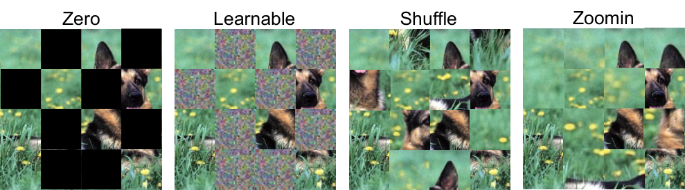
Table 10: Ablation on reducing the difficulty of the pretext task. We report the top-1 accuracy on ImageNet-1K for each approach with different pretraining epochs. Ours w/o unmixing denotes that we do not reduce the difficulty of the pretext task. Details of the other two approaches are described in Section 3.3.

Content to filling. While MixMAE default fills the masked tokens of one image with visible tokens from another image, we also explore more design choices. Specifically, we try to fill the masked tokens with the following contents.

•

Zero: Filling the masked tokens with zeros. This approach causes serious mismatches between the masked tokens and the visible tokens.
•

Learnable: Following previous works beit; simmim, we fill the masked tokens with a shared learnable token. The difference between the zero approach is that learnable tokens can be adapted to visible tokens to match the distribution of the training set.
•

Shuffle: We randomly shuffle the masked tokens, and then fill the masked locations with the shuffled tokens. We note that this approach is similar to solving jigsaw puzzles jigsaw with the difference that we need to fully regress the pixels.
•

Zoomin: We zoom in the original image and randomly crop an image patch with the size of the original image. We then fill the masked tokens with tokens from the cropped image. This approach also provides masking tokens that are similar to visible ones but is harder than the shuffle approach.

We visualize the four approaches in Figure 4. We compare the performances of the four approaches in Table 9. Our default choice Mix performs best in terms of accuracy on ImageNet-1K and mIoU on ADE20K. We find the learnable approach has a similar performance on ImageNet-1K but better performance on ADE20K compared to Zero. We hypothesize that the training-finetuning inconsistency has a larger impact on tasks without a lot of labeled images. The shuffle and zoomin approaches perform much worse than other approaches. Those two strategies cause easier pretext task and have lower pretraining loss. However, the learned representation quality is lower.

Dual reconstruction. We ablate the proposed dual reconstruction in Table 9. We find that dual reconstruction greatly boosts the performance on downstream tasks. The performance gap is larger on ADE20K, where we observe +2.6 mIoU with the dual reconstruction. Note that the computation overhead of dual reconstruction is negligible as the decoder is lightweight.

Masking ratio. Our MixMAE implements different masking ratios by mixing more images at inputs. In addition, we also experiment to add $\mathrm{[MASK]}$ tokens for a higher masking ratio. We ablate the masking ratios in Table 9. We find that using a masking ratio 75% by mixing 4 images performs best. In contrast, adding $\mathrm{[MASK]}$ tokens for a 75% masking ratio has worse performance, demonstrating the effectiveness of the proposed mixing approach.

Pretraining epochs. Thanks to the dual reconstruction, our MixMAE can achieve strong performance with few pretraining epochs. We ablate the pretraining epochs in Table 9. We find that the mIoU on ADE20K can be further improved with more pretraining epochs. We achieve 51.0 mIoU with 900 epochs of pretraining. In contrast, the accuracy on ImageNet-1K does not improve after 600 epochs. It might be because the finetuning on ImageNet-1K is more adequate.

Reducing the difficulty. As stated in Section 3.3, directly performing reconstruction with the mixed input is a much more challenging optimization problem. Hence, we provide two practical approaches to reduce the difficulty. We ablate the design in Table 10. We note that all the approaches do not bring nonnegligible FLOPs or parameters. We find that the performance of the approach without unmixing is worst even when trained for more epochs. In contrast, using mix embedding alleviates the problem and improves its performance with longer pretraining. However, using masked self-attention in our final solution is much more efficient, and has better performance.

7 Discussion and Conclusion

This paper proposes Mixed and Masked AutoEncoder (MixMAE) for efficient visual representation learning. Our MixMAE uses a mixed input created by mixing two (or more) images with random masks, and applies dual reconstruction to recover the original two (or more) images from the mixed hidden representations. We further explore using Swin Transformer with a larger window size for efficient representation learning. Empirical results on 7 visual benchmarks demonstrate MixMAE can learn high-quality visual representations efficiently and has better FLOPs / performance tradeoff than previous MIM works. While this paper focuses on the vision field, we hope our work will inspire future works in other modalities, such as text and audio.

Acknowledgement

This project is funded in part by National Key R&D Program of China Project 2022ZD0161100, by the Centre for Perceptual and Interactive Intelligence (CPII) Ltd under the Innovation and Technology Commission (ITC)’s InnoHK, by General Research Fund of Hong Kong RGC Project 14204021. Hongsheng Li is a PI of CPII under the InnoHK.

References

(1) Jean-Baptiste Alayrac, Joao Carreira, and Andrew Zisserman. The visual centrifuge: Model-free layered video representations. In CVPR, 2019.
(2) Sara Atito, Muhammad Awais, and Josef Kittler. Sit: Self-supervised vision transformer. arXiv:2104.03602, 2021.
(3) Alexei Baevski, Wei-Ning Hsu, Qiantong Xu, Arun Babu, Jiatao Gu, and Michael Auli. Data2vec: A general framework for self-supervised learning in speech, vision and language. arXiv:2202.03555, 2022.
(4) Hangbo Bao, Li Dong, and Furu Wei. Beit: Bert pre-training of image transformers. In ICLR, 2021.
(5) Mathilde Caron, Hugo Touvron, Ishan Misra, Hervé Jégou, Julien Mairal, Piotr Bojanowski, and Armand Joulin. Emerging properties in self-supervised vision transformers. In ICCV, 2021.
(6) Mark Chen, Alec Radford, Rewon Child, Jeffrey Wu, Heewoo Jun, David Luan, and Ilya Sutskever. Generative pretraining from pixels. In ICML, 2020.
(7) Xiaokang Chen, Mingyu Ding, Xiaodi Wang, Ying Xin, Shentong Mo, Yunhao Wang, Shumin Han, Ping Luo, Gang Zeng, and Jingdong Wang. Context autoencoder for self-supervised representation learning. arXiv:2202.03026, 2022.
(8) Xinlei Chen, Saining Xie, and Kaiming He. An empirical study of training self-supervised vision transformers. In ICCV, 2021.
(9) Xiangxiang Chu, Zhi Tian, Yuqing Wang, Bo Zhang, Haibing Ren, Xiaolin Wei, Huaxia Xia, and Chunhua Shen. Twins: Revisiting the design of spatial attention in vision transformers. NeurIPS, 34:9355–9366, 2021.
(10) Kevin Clark, Minh-Thang Luong, Quoc V Le, and Christopher D Manning. Electra: Pre-training text encoders as discriminators rather than generators. In ICLR, 2020.
(11) Ekin D Cubuk, Barret Zoph, Jonathon Shlens, and Quoc V Le. Randaugment: Practical automated data augmentation with a reduced search space. In CVPRW, 2020.
(12) Zihang Dai, Hanxiao Liu, Quoc V Le, and Mingxing Tan. Coatnet: Marrying convolution and attention for all data sizes. NeurIPS, 34:3965–3977, 2021.
(13) Jia Deng, Wei Dong, Richard Socher, Li-Jia Li, K. Li, and Li Fei-Fei. Imagenet: A large-scale hierarchical image database. In CVPR, 2009.
(14) Jacob Devlin, Ming-Wei Chang, Kenton Lee, and Kristina Toutanova. Bert: Pre-training of deep bidirectional transformers for language understanding. In NAACL, 2019.
(15) Xiaoyi Dong, Jianmin Bao, Ting Zhang, Dongdong Chen, Weiming Zhang, Lu Yuan, Dong Chen, Fang Wen, and Nenghai Yu. Peco: Perceptual codebook for bert pre-training of vision transformers. arXiv:2111.12710, 2021.
(16) Alexey Dosovitskiy, Lucas Beyer, Alexander Kolesnikov, Dirk Weissenborn, Xiaohua Zhai, Thomas Unterthiner, Mostafa Dehghani, Matthias Minderer, Georg Heigold, Sylvain Gelly, Jakob Uszkoreit, and Neil Houlsby. An image is worth 16x16 words: Transformers for image recognition at scale. In ICLR, 2021.
(17) Golnaz Ghiasi, Yin Cui, Aravind Srinivas, Rui Qian, Tsung-Yi Lin, Ekin D Cubuk, Quoc V Le, and Barret Zoph. Simple copy-paste is a strong data augmentation method for instance segmentation. In CVPR, 2021.
(18) Xavier Glorot and Yoshua Bengio. Understanding the difficulty of training deep feedforward neural networks. In AISTATS, 2010.
(19) Priya Goyal, Piotr Dollár, Ross Girshick, Pieter Noordhuis, Lukasz Wesolowski, Aapo Kyrola, Andrew Tulloch, Yangqing Jia, and Kaiming He. Accurate, large minibatch sgd: Training imagenet in 1 hour. arXiv:1706.02677, 2017.
(20) Raghav Goyal, Samira Ebrahimi Kahou, Vincent Michalski, Joanna Materzynska, Susanne Westphal, Heuna Kim, Valentin Haenel, Ingo Fründ, Peter N. Yianilos, Moritz Mueller-Freitag, Florian Hoppe, Christian Thurau, Ingo Bax, and Roland Memisevic. The “something something” video database for learning and evaluating visual common sense. In ICCV, 2017.
(21) Kaiming He, Xinlei Chen, Saining Xie, Yanghao Li, Piotr Doll’ar, and Ross B. Girshick. Masked autoencoders are scalable vision learners. In CVPR, 2021.
(22) Kaiming He, Georgia Gkioxari, Piotr Dollár, and Ross Girshick. Mask r-cnn. In ICCV, 2017.
(23) Grant Van Horn, Oisin Mac Aodha, Yang Song, Yin Cui, Chen Sun, Alexander Shepard, Hartwig Adam, Pietro Perona, and Serge J. Belongie. The inaturalist species classification and detection dataset. In CVPR, 2018.
(24) Gao Huang, Yu Sun, Zhuang Liu, Daniel Sedra, and Kilian Q Weinberger. Deep networks with stochastic depth. In ECCV, 2016.
(25) Lang Huang, Shan You, Mingkai Zheng, Fei Wang, Chen Qian, and Toshihiko Yamasaki. Green hierarchical vision transformer for masked image modeling. arXiv preprint arXiv:2205.13515, 2022.
(26) Alexander Kolesnikov, Lucas Beyer, Xiaohua Zhai, Joan Puigcerver, Jessica Yung, Sylvain Gelly, and Neil Houlsby. Big transfer (bit): General visual representation learning. In ECCV, 2020.
(27) Chunyuan Li, Jianwei Yang, Pengchuan Zhang, Mei Gao, Bin Xiao, Xiyang Dai, Lu Yuan, and Jianfeng Gao. Efficient self-supervised vision transformers for representation learning. In ICLR, 2022.
(28) Xiang Li, Wenhai Wang, Lingfeng Yang, and Jian Yang. Uniform masking: Enabling mae pre-training for pyramid-based vision transformers with locality. arXiv:2205.10063, 2022.
(29) Yanghao Li, Saining Xie, Xinlei Chen, Piotr Dollar, Kaiming He, and Ross Girshick. Benchmarking detection transfer learning with vision transformers. arXiv:2111.11429, 2021.
(30) Tsung-Yi Lin, Piotr Dollár, Ross Girshick, Kaiming He, Bharath Hariharan, and Serge Belongie. Feature pyramid networks for object detection. In CVPR, 2017.
(31) Tsung-Yi Lin, Michael Maire, Serge J. Belongie, James Hays, Pietro Perona, Deva Ramanan, Piotr Dollár, and C. Lawrence Zitnick. Microsoft coco: Common objects in context. In ECCV, 2014.
(32) Guilin Liu, Kevin J Shih, Ting-Chun Wang, Fitsum A Reda, Karan Sapra, Zhiding Yu, Andrew Tao, and Bryan Catanzaro. Partial convolution based padding. arXiv:1811.11718, 2018.
(33) Jihao Liu, Xin Huang, Guanglu Song, Hongsheng Li, and Yu Liu. Uninet: Unified architecture search with convolution, transformer, and mlp. In ECCV, pages 33–49. Springer, 2022.
(34) Jihao Liu, Boxiao Liu, Hang Zhou, Hongsheng Li, and Yu Liu. Tokenmix: Rethinking image mixing for data augmentation in vision transformers. In ECCV, pages 455–471. Springer, 2022.
(35) Ze Liu, Han Hu, Yutong Lin, Zhuliang Yao, Zhenda Xie, Yixuan Wei, Jia Ning, Yue Cao, Zheng Zhang, Li Dong, et al. Swin transformer v2: Scaling up capacity and resolution. In CVPR, pages 12009–12019, 2022.
(36) Ze Liu, Yutong Lin, Yue Cao, Han Hu, Yixuan Wei, Zheng Zhang, Stephen Lin, and Baining Guo. Swin transformer: Hierarchical vision transformer using shifted windows. In ICCV, 2021.
(37) Ilya Loshchilov and Frank Hutter. Sgdr: Stochastic gradient descent with warm restarts. In ICLR, 2016.
(38) Ilya Loshchilov and Frank Hutter. Decoupled weight decay regularization. In ICLR, 2017.
(39) Mehdi Noroozi and Paolo Favaro. Unsupervised learning of visual representations by solving jigsaw puzzles. In ECCV, 2016.
(40) Aditya Ramesh, Mikhail Pavlov, Gabriel Goh, Scott Gray, Chelsea Voss, Alec Radford, Mark Chen, and Ilya Sutskever. Zero-shot text-to-image generation. In ICML, 2021.
(41) Jason Tyler Rolfe. Discrete variational autoencoders. In ICLR, 2016.
(42) Chen Sun, Abhinav Shrivastava, Saurabh Singh, and Abhinav Gupta. Revisiting unreasonable effectiveness of data in deep learning era. In ICCV, 2017.
(43) Christian Szegedy, Vincent Vanhoucke, Sergey Ioffe, Jon Shlens, and Zbigniew Wojna. Rethinking the inception architecture for computer vision. In CVPR, 2016.
(44) Zhan Tong, Yibing Song, Jue Wang, and Limin Wang. Videomae: Masked autoencoders are data-efficient learners for self-supervised video pre-training. arXiv:2203.12602, 2022.
(45) Ashish Vaswani, Noam Shazeer, Niki Parmar, Jakob Uszkoreit, Llion Jones, Aidan N Gomez, Łukasz Kaiser, and Illia Polosukhin. Attention is all you need. NeurIPS, 30, 2017.
(46) Wenhai Wang, Enze Xie, Xiang Li, Deng-Ping Fan, Kaitao Song, Ding Liang, Tong Lu, Ping Luo, and Ling Shao. Pyramid vision transformer: A versatile backbone for dense prediction without convolutions. In ICCV, 2021.
(47) Chen Wei, Haoqi Fan, Saining Xie, Chao-Yuan Wu, Alan Yuille, and Christoph Feichtenhofer. Masked feature prediction for self-supervised visual pre-training. arXiv:2112.09133, 2021.
(48) Yixuan Wei, Han Hu, Zhenda Xie, Zheng Zhang, Yue Cao, Jianmin Bao, Dong Chen, and Baining Guo. Contrastive learning rivals masked image modeling in fine-tuning via feature distillation. arXiv:2205.14141, 2022.
(49) Tete Xiao, Yingcheng Liu, Bolei Zhou, Yuning Jiang, and Jian Sun. Unified perceptual parsing for scene understanding. In ECCV, 2018.
(50) Tete Xiao, Ilija Radosavovic, Trevor Darrell, and Jitendra Malik. Masked visual pre-training for motor control. arXiv:2111.11429, 2022.
(51) Zhenda Xie, Zheng Zhang, Yue Cao, Yutong Lin, Jianmin Bao, Zhuliang Yao, Qi Dai, and Han Hu. Simmim: A simple framework for masked image modeling. In CVPR, 2021.
(52) Sangdoo Yun, Dongyoon Han, Seong Joon Oh, Sanghyuk Chun, Junsuk Choe, and Youngjoon Yoo. Cutmix: Regularization strategy to train strong classifiers with localizable features. In ICCV, 2019.
(53) Sangdoo Yun, Dongyoon Han, Seong Joon Oh, Sanghyuk Chun, Junsuk Choe, and Youngjoon Yoo. Cutmix: Regularization strategy to train strong classifiers with localizable features. In ICCV, 2019.
(54) Hongyi Zhang, Moustapha Cisse, Yann N Dauphin, and David Lopez-Paz. mixup: Beyond empirical risk minimization. In ICLR, 2017.
(55) Bolei Zhou, Àgata Lapedriza, Jianxiong Xiao, Antonio Torralba, and Aude Oliva. Learning deep features for scene recognition using places database. In NeurIPS, 2014.
(56) Bolei Zhou, Hang Zhao, Xavier Puig, Sanja Fidler, Adela Barriuso, and Antonio Torralba. Scene parsing through ade20k dataset. In CVPR, 2017.
(57) Jinghao Zhou, Chen Wei, Huiyu Wang, Wei Shen, Cihang Xie, Alan Yuille, and Tao Kong. ibot: Image bert pre-training with online tokenizer. In ICLR, 2021.

Appendix A Training Details

A.1 Hyperparameters of Pretraining and Finetuning

We include details about the hyperparameters for reimplementation.

Pretraining. The default setting is in Table 11. We use xavier_uniform xavier to initialize all Transformer blocks following original ViT vit. We by default use batch size of 1024 and scale the learning rate with linear rule goyal2017accurate: lr=base_lr $\times$ batch_size / 256.

config	value
optimizer	AdamW adamw
base learning rate	$1.5\times 10^{-4}$
weight decay	0.05
optimizer momentum	$\beta_{1},\beta_{2}$ =0.9,0.95 igpt
learning rate schedule	cosine decay cosine
warmup epochs	40
augmentation	RandomResizedCrop

Table 11: Pretraining on ImageNet-1K.

Finetuning on ImageNet-1K. The default setting is in Table 12. We use layer-wise learning rate decay following beit; electra. The decay ratio is swept in {0.7, 0.75, 0.8}, and we find 0.7 performs best. Following pretraining, the learning rate is scaled with linear rule: lr=base_lr $\times$ batch_size / 256.

config	value
optimizer	AdamW
base learning rate	$5\times 10^{-4}$
layer-wise lr decay beit; electra	0.7
batch size	1024
weight decay	0.05
optimizer momentum	$\beta_{1},\beta_{2}$ =0.9,0.999
learning rate schedule	cosine decay
warmup epochs	5
training epochs	100 (B), 50 (L/H)
augmentation	RandAug(9, 0.5) randaug
LabelSmooth inception	0.1
Mixup zhang2017mixup	0.8
CutMix yun2019cutmix	1.0
drop path droppath	0.15 (B), 0.2 (L), 0.3 (H)

Table 12: Finetuning on ImageNet-1K.

Finetuning on other classification datasets. We reuse the setting in Table 12. We adjust the drop path rate for each dataset.

Finetuning on COCO. We use the Mask RCNN he2017mask framework with the encoder of MixMAE as its backbone. We follow the training setting in vitdet; mae. In particular, we use large-scale jitter lsj augmentation with 1024 $\times$ 1024 resolution and [0.1, 2.0] scale range. We use step learning rate schedule with 0.25 epochs of warmup. We finetune Swin-B/-L for 55/80 epochs. We use a layer-wise learning rate and set the decay ratio to 0.85/0.9 for Swin-B/-L.

Finetuning on ADE20K. We use the UperNet upernet framework with the encoder of MixMAE as its backbone. We finetune for 16K iterations with a batch size of 16. We use the layer-wise learning rate and set the decay ratio to 0.85/0.9 for Swin-B/-L. We adopt others settings from BEiT beit.

A.2 Additional Results of Ablation Studies

A.2.1 Ablation results on COCO

We show more results of our ablation studies on COCO benchmark in Table 14 14 16 16. We find that the performance on the COCO is similar to that on ADE20K.

Type	AP^box	AP^mask
Mix	51.5	45.9
Zero	51.0	45.3
Learnable	50.9	45.1
Shuffle	46.5	41.6
Zoomin	47.9	42.6

Table 13: Filling content.

# Images (ratio)	AP^box	AP^mask
2 (0.5)	51.5	45.9
2 w/ $\mathrm{[M]}$ (0.75)	51.2	45.4
3 (0.67)	51.6	45.9
4 (0.75)	52.3	46.4
5 (0.8)	51.4	45.4

Table 14: Number of mixing images.

# Epochs	AP^box	AP^mask
300	51.5	45.9
600	52.2	46.5
900	52.4	46.7

Table 15: Pretraining epochs.

Dual	AP^box	AP^mask
✓	51.5	45.9
✗	50.0	44.4

Table 16: Dual reconstruction.

Method	Backbone	Pretrain Epochs	Top-1 Acc.
Supervised	ViT-B	-	81.8
MAE	ViT-B	1600	83.6
BEiT	ViT-B	800	83.2
MixMAE	ViT-B	600	83.8

Table 17: Performance of MixMAE and other methods on ViT.

A.2.2 Pretraining Time Comparison

We compare the wall-clock time of the pretrain in Table 18. The pretrain time is measured on 8 NVIDIA-A100-SXM-80GB GPUs with a total batch size of 1024.

Method	Backbone	Pretrain epochs	Pretrain Time (GPU hours)	Top-1 Acc.
SimMIM simmim	Swin-B	800	116	84.0
MAE mae	ViT-B	1600	123	83.6
BEiT beit	ViT-B	800	151	83.2
MixMAE	Swin-B	600	85	84.6
MixMAE	Swin-B/W14	300	64	84.8
MixMAE	Swin-B/W14	600	127	85.1

Table 18: Wall-clock time comparison of MIM methods.

A.2.3 Performance on ViT.

We show the results on ViT vit in Table 17.

Figure 5: Mixed convolution.

Method	Backbone	Input Size	Pretrain Data	Top-1 Acc.
BiT-S bit	Res50x3	$448\times 448$	ImageNet-1K	80.0
BiT-M bit	Res50x3	$448\times 448$	ImageNet-21K	84.0
MixMAE	Res50x3	$224\times 224$	ImageNet-1K (w/o labels)	81.8
BiT-S bit	Res101x3	$448\times 448$	ImageNet-1K	80.3
BiT-M bit	Res101x3	$448\times 448$	ImageNet-21K	84.3
MixMAE	Res101x3	$224\times 224$	ImageNet-1K (w/o labels)	82.6

Table 19: Results on ConvNets. All results of MixMAE are obtained by pretraining for 300 epochs and finetuning for 100 epochs on ImageNet-1K. We report the top-1 accuracy on ImageNet-1K.

A.3 Extend to ConvNets

While our MixMAE uses a hierarchical Transformer as the encoder, we also explore popular ConvNets. In particular, we use ResNet50x3 and ResNet101x3 as the encoder and compare the finetuning results on ImageNet-1K with BiT bit. To reduce the difficulty of the pretext task, we extend the idea of partial convoluation partialconv and propose a mixed version, as illustrated in Figure 5.

We compare the results in Table 19. In particular, our MixMAE outperforms BiT-S by a large margin with half the input size. We note that BiT-M achieves better results by pretraining with 10 $\times$ larger dataset ImageNet-21K. We believe the results of MixMAE can be further improved by using much larger datasets as shown by beit, and we leave it as future work.